


Abstract
We explore the evolution of the different ejecta components generated during the merger of a neutron star and a black hole. Our focus is the interplay between material ejected dynamically during the merger, and the wind launched on a viscous time-scale by the remnant accretion disc. These components are expected to contribute to an electromagnetic transient and to produce r-process elements, each with a different signature when considered separately. Here we introduce a two-step approach to investigate their combined evolution, using two- and three-dimensional hydrodynamic simulations. Starting from the output of a merger simulation, we identify each component in the initial condition based on its phase-space distribution, and evolve the accretion disc in axisymmetry. The wind blown from this disc is injected into a three-dimensional computational domain where the dynamical ejecta is evolved. We find that the wind can suppress fallback accretion on time-scales longer than ∼100 ms. Because of self-similar viscous evolution, the disc accretion at late times nevertheless approaches a power-law time dependence ∝t−2.2. This can power some late-time gamma-ray burst engine activity, although the available energy is significantly less than in traditional fallback models. Inclusion of radioactive heating due to the r-process does not significantly affect the fallback accretion rate or the disc wind. We do not find any significant modification to the wind properties at large radius due to interaction with the dynamical ejecta. This is a consequence of the different expansion velocities of the two components.
1 INTRODUCTION
Double neutron star (NS) or NS–black hole (BH) mergers are among the main candidates for direct detection of gravitational waves by advanced ground-based laser interferometers (Abadie et al. 2010). The ejecta from these mergers are also a prime candidate for the generation of r-process elements (e.g. Lattimer & Schramm 1974; Freiburghaus, Rosswog & Thielemann 1999; Goriely et al. 2013). Radioactive decay of these elements is expected to power an electromagnetic counterpart that can aid in the localization of the gravitational wave source (Li & Paczyński 1998; Metzger et al. 2010b). Finally, these mergers are the leading candidate progenitor for short-duration gamma-ray bursts (SGRBs; see e.g. Berger 2014 for a recent review).
The ejection of material by tidal forces during the merger depends on a number of factors, including the mass ratio of the binary, the spin of each component, and the properties of the nuclear equation of state (e.g. Bauswein, Goriely & Janka 2013; Kyutoku, Ioka & Shibata 2013). In BH–NS mergers, the amount of ejecta also depends crucially on BH spin (e.g. Foucart 2012). The gravitationally bound part of this dynamical ejecta leads to fallback accretion on to the BH. Because fallback extends over time-scales much longer than the viscous time of the disc, it has been proposed as a source of extended prompt emission and/or X-ray flares in the afterglows of some SGRBs (Faber et al. 2006; Gehrels et al. 2006; Rosswog 2007). However, the gravitational binding energy of material accreting on time-scales longer than ∼1 s is comparable to or less than the energy injected by radioactive heating during r-process nucleosynthesis. Thus fallback accretion can potentially be suppressed when this heating is taken into account (Metzger et al. 2010a).
Furthermore, the dynamical ejecta do not exist in isolation. The accretion disc formed during the merger is an additional source of material in two ways. First, on ∼100 ms time-scales, material can be unbound by neutrino energy deposition in a broad polar outflow (the neutrino-driven wind; McLaughlin & Surman 2005; Surman, McLaughlin & Hix 2006; Surman et al. 2008; Dessart et al. 2009; Wanajo & Janka 2012; Metzger & Fernández 2014; Perego et al. 2014). Second, over longer, ∼1 s time-scales, energy deposition by angular momentum transport and nuclear recombination together with decreased neutrino cooling lead to substantial mass ejection in a quasi-spherical outflow (a freezout wind; Lee, Ramirez-Ruiz & López-Cámara 2009; Metzger, Piro & Quataert 2009; Fernández & Metzger 2013a; Metzger & Fernández 2014; Fernández et al. 2015; Just et al. 2015). The amount of material ejected by these two disc channels can be comparable to that in the dynamical ejecta, although its composition is expected to be less neutron rich, with observable consequences for the ensuing kilonova transient (Barnes & Kasen 2013; Kasen, Badnell & Barnes 2013; Tanaka & Hotokezaka 2013; Tanaka et al. 2014, see also Kasen, Fernández & Metzger 2014).
While the dynamical ejecta are generally launched earlier and is faster than disc outflows, the interaction between these two components can be non-trivial. First, disc winds can modify fallback accretion relative to what is expected from purely ballistic trajectories. Conversely, part or all of the disc wind can mix with slower moving components of the dynamical ejecta, potentially leading to different nucleosynthetic and electromagnetic signatures than predicted from the wind alone.
In this paper we examine the interplay between these components by means of two-dimensional (2D) and three-dimensional (3D) hydrodynamic simulations. Given that evolving the complete system over the time-scales of interest with all the relevant physics is computationally expensive, we develop a two-stage modelling approach that takes advantage of the spatial and temporal decoupling of key processes. Starting from the output of a BH+NS merger simulation, we evolve the remnant accretion disc in axisymmetry (2D), with and without the dynamical ejecta, and including neutrino and viscous processes. This leads to the production of an axisymmetric disc wind. This wind is then sampled at a radius that approximately separates the accretion disc from the non-axisymmetric dynamical ejecta. The sampled wind is then injected into a larger, 3D computational domain with an inner boundary that coincides with the wind sampling radius, and in which the dynamical ejecta is evolved. Our goal is to identify the key processes that govern the interaction between these two ejecta components using approximate modelling of the physics. Future studies will refine this analysis.
The paper is organized as follows. Section 2 describes the numerical approach employed, including the separation of the system into different ejecta components. Section 3 presents our results, including the properties of the disc wind in 2D, the properties of fallback accretion without wind, and the interplay between these two components. Our results are summarized in Section 4, where broader observational implications are also discussed.
2 COMPUTATIONAL METHODOLOGY
It is infeasible to evolve the combined accretion disc plus dynamical ejecta system with all the relevant physics in 3D for the time-scales of interest (∼10 s). In particular, explicit viscous angular momentum transport requires resolving the corresponding diffusion time-scale on the smallest grid cells in the simulation.
Fortunately, the (non-axisymmetric) dynamical ejecta is mostly spatially decoupled from the (largely axisymmetric) accretion disc once the initial transient phase ends, a few dynamical times after the merger. Angular momentum transport and neutrino processes operate on time-scales slower than the expansion time outside radii ∼108 cm (Section 2.3), so they can be neglected in these regions to first approximation.
We thus adopt a two-stage approach to model the interaction of wind and dynamical ejecta. First, we evolve the system in axisymmetry including viscous and neutrino source terms, and measure the properties of the resulting disc wind at a radius that separates the two components. We then evolve the dynamical ejecta in 3D, using a computational domain that has its inner radial boundary at the radius where the wind properties were determined. From this inner boundary, the wind is injected into the domain. The only source terms employed in this second step are gravity and radioactive heating, leading to significant savings in computational time.
In what follows, we describe the numerical method used to evolve the hydrodynamic equations (Section 2.1), the initial conditions, including how we identify and separate distinct components of the merger remnant (Section 2.2), the sampling and injection of the wind in 3D models (Section 2.3), and the list of models simulated (Section 2.4).
2.1 Time-dependent hydrodynamics
The equations of hydrodynamics are solved numerically with the dimensionally split PPM solver in Flash|${\scriptstyle 3.2}$| (Fryxell et al. 2000; Dubey et al. 2009). The public version of the code has been modified to include a non-uniformly spaced grid (Fernández 2012), and physical source terms needed to model the evolution of merger remnant accretion discs (Fernández & Metzger 2013a,b; Metzger & Fernández 2014; Fernández et al. 2015). The equation of state is that of Timmes & Swesty (2000), with abundances of neutrons, protons, and alpha particles in nuclear statistical equilibrium. The nuclear binding energy contribution from alpha particles is included.
The 2D version of the code solves the equations of mass-, poloidal momentum-, angular momentum-, energy-, and lepton number conservation in spherical polar coordinates (r, θ). Source terms include angular momentum transport by an anomalous shear stress using the kinematic viscosity of Shakura & Sunyaev (1973), and neutrino source terms via a leakage scheme that only includes charge–current weak interactions (Metzger & Fernández 2014).
The 3D implementation solves the equations of hydrodynamics in spherical polar coordinates (r, θ, ϕ) with gravity and radioactive heating as the only source terms. The split PPM version of Flash|${\scriptstyle 3.2}$| requires minor modifications to be extended to 3D spherical coordinates. A description of these modifications and tests of the implementation will be presented elsewhere. We employ the analytic parametrization of r-process radioactive heating from Korobkin et al. (2012). This source term is included in order to qualitatively assess the effect of radioactive heating on the dynamics; details such as its sensitivity to the electron fraction and spatial location are ignored. This source term is applied in cells that have temperature T < 5 × 10⁹ K.
In all models, we approximate the gravitational potential of a spinning BH via the pseudo-Newtonian potential of Artemova, Bjoernsson & Novikov (1996). The main advantage of this potential is that it reproduces the location of the innermost stable circular orbit (ISCO) of the Kerr metric, and leads to steady-state, thin, sub-Eddington accretion disc solutions to within ∼10–20 per cent of the exact relativistic value as computed by Artemova et al. (1996). The implied space–time is spherically symmetric, however, so while convenient for computational purposes, it is not a very accurate approximation for all space if the spin parameter is high. Nevertheless, since most of the material that resides at radii close to the BH – where general relativistic (GR) effects are the strongest – lies mostly on the midplane, we consider this choice of potential as an acceptable approximation for the inner disc dynamics. At the radii where the phenomena we are interested in occur (r ≳ 108 cm), GR effects are very weak (few per cent or less).
The computational domain is discretized logarithmically in radius, uniformly in cos θ along the polar direction, and uniformly in azimuth. The resolution is 64 cells per decade in radius, 56 cells meridionally from θ = 0 to θ = π, and 192 cells for ϕ ∈ [0, 2π]. At the equator, cells are such that Δr/r ≃ Δθ ≃ Δϕ ≃ 2°. The (r, θ) resolution is the same for most 2D and 3D models, the exception being a 2D model run at double resolution to check for convergence.
In 2D models that include the inner disc evolution, the domain covers the full range of polar angles, and extends from a radius halfway between the BH horizon and the ISCO, until a radius 1000 times larger. The radial limits of 3D models are the wind injection radius rcut (Section 2.2) on the inside, and a radius 104 times larger on the outside.
The boundary conditions are reflecting in θ and periodic in ϕ. In 2D and 3D models with no wind injection, both radial boundaries allow mass to leave the domain (see e.g. Fernández & Metzger 2013a for details). When a wind is injected into a 3D model, the default boundary condition involves solution of a Riemann problem. This procedure is discussed in Section 2.3.
2.2 Initial condition and separation of components
The initial condition is obtained from the output of a Newtonian smoothed particle hydrodynamic (SPH) simulation of the merger of a 10 M⊙ BH with a 1.4 M⊙ NS reported in Rosswog, Piran & Nakar (2013). This BH mass is close to (but somewhat higher than) the peak of the inferred stellar mass BH distribution in the galaxy (e.g. Özel et al. 2010; Farr et al. 2011). The simulations use the Shen et al. (1998) equation of state, a multiflavour, energy-integrated neutrino leakage scheme (Rosswog & Liebendörfer 2003), and Newtonian gravity with an absorbing boundary condition at the Schwarzschild radius of the (non-spinning) BH. The time of the snapshot corresponds to 139 ms after the merger.
The SPH data are mapped into the Eulerian grid using the appropriate smoothing kernel to reconstruct conserved quantities from the particle distribution. In the case of 2D simulations, data are axisymmetrized by computing azimuthal averages of conserved quantities (e.g. the radial velocity is given by 〈vr〉 = ∫(ρvr)dV/∫ρdV, with dV the volume of the cells included in the average). We use the density, temperature, and electron fraction to reconstruct the rest of the thermodynamic variables using our equation of state. If the temperature is below 5 × 10⁹ K, we assume full recombination into alpha particles (e.g. if Ye < 0.5, the alpha mass fraction is set to 2Ye and the proton fraction to zero).
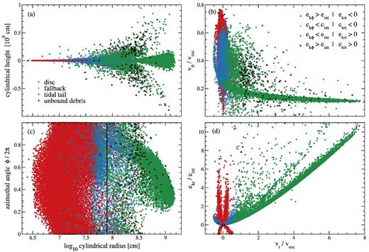
Phase-space distribution of particles that comprise the initial state of the system. The disc (red solid circles), fallback (blue open circles), tidal tail (green filled circles), and unbound debris (black triangles) components are separated according to the sign of their total specific energy etot, and the ratio of the kinetic energy in the ϕ direction ekϕ to the internal energy eint, as indicated in panel (b). The vertical line in panel (c) indicates the radius rcut at which the disc wind properties are measured from 2D simulations. This radius marks the inner radial boundary of 3D models.
We identify four components in the system.
Disc: gravitationally bound (etot < 0) and rotationally supported (ekϕ > eint). This is the innermost component in radius and nearly axisymmetric, as shown in Figs 1(a) and (c), containing most of the mass (0.2 M⊙).
Tidal tail: gravitationally unbound and with ekϕ < eint. The energy is dominated by the radial kinetic energy, as shown in Fig. 1, comprising a highly localized structure in phase space, outermost in radius. The mass in this component is 0.06 M⊙.
Fallback: gravitationally bound, and primarily gas pressure supported (ekϕ < eint). With this definition, it includes the outermost part of the disc and the innermost part of the tidal tail, as shown most explicitly in Fig. 1(b). The mass in this component is 0.02 M⊙.
Unbound debris: the remaining material is gravitationally unbound with significant rotation. It can be considered part of the dynamical ejecta, but it does not comprise as localized a structure as the tidal tail. The mass is ∼10−3 M⊙.
We follow the separate evolution of these components in our Flash simulations using passive scalars, constructed by taking the ratio of the partial mass density formed with each subgroup of SPH particles to the total mass density. By definition, these scalars add up to unity.
Once mapped into Flash, these components are not completely decoupled, however. Figs 1(a) and (c) show that there is spatial overlap between the particles, particularly around r ∼ 108 cm. This overlap leads to mixing when reconstructing the fluid distribution using the SPH kernel. Approximately 0.01 M⊙ of material initially tagged as tidal tail is gravitationally bound, while a very small amount of disc and fallback material (≃10−3 M⊙ in total) is unbound.
We choose a radius rcut = 800 km to quantify the unbound properties of the disc wind in 2D axisymmetric simulations of the inner disc. This position corresponds approximately to the innermost edge of the tidal tail (Fig. 1c), separating a nearly axisymmetric matter distribution on the inside from a highly non-axisymmetric one on the outside. At the time of our initial conditions (139 ms after the merger), this surface encloses 99 per cent of the disc mass and 43 per cent of the fallback mass.
The mass of the BH at the beginning of the simulation is approximately 11.1 M⊙, and it is kept fixed thereafter. The inner boundary for 2D models is set at 3.7 × 106 cm, midway between the ISCO and the event horizon of a BH with spin parameter a = 0.8. A significantly smaller spin would be inconsistent with the tidal disruption of the NS (e.g. Foucart 2012). Also, the potential of Artemova et al. (1996) asymptotes to Newtonian for very high spins, so this choice is more consistent with the physics used to generate the initial condition (a BH modelled as a Newtonian point mass with an absorbing boundary condition at the Schwarzschild radius of a non-spinning BH; Rosswog et al. 2013).
2.3 Wind injection in 3D simulations
In 2D simulations, we record the properties of the material crossing at r = rcut, as a function of polar angle and at regular time intervals. Subsequent injection of this data into 3D models is achieved by interpolating the recorded variables in time for a given polar angle, copying the resulting values for all azimuthal angles.
The inner radial ghost cells of 3D models are filled by solving a Riemann problem at the inner radial boundary, taking as left-hand state the quantities interpolated from the sampled wind, and as right-hand state the innermost active cell in radius. This is done to account for the possibility that fallback may carry a larger momentum flux than the wind along certain directions. For operational simplicity, we employ the HLLC solver of Toro, Spruce & Speares (1994), which does not require any iterations. As a check, we run a model that simply copies the interpolated values from the 2D simulations into the ghost cells of the 3D domain, without a Riemann solution.
In all cases, if the resulting radial velocity at the ghost cells is negative, a standard outflow boundary condition is adopted: the ghost cells are filled with data from the innermost active cell.
2.4 Models evolved
Table 1 summarizes our simulations. We run three sets: one that evolves the complete system in 2D with all the physics (C-series, for ‘complete’), one that investigates fallback accretion without wind (F-series, for ‘fallback’), and one that evolves the dynamical ejecta with wind injection from the inner radial boundary (I-series, for ‘injection’).
Models evolved and summary of results. The first six models follow the evolution of the system in 2D, including all components (C2d, C2d-res, C2d-src, C2d-h), material interior to 800 km (C2d-df), or just disc material (C2d-d). The second four models explore the properties of fallback accretion in 2D (F2d, F2d-h) and 3D (F3d, F3d-h) neglecting the disc wind. The final five models investigate the effect of injecting the disc wind measured in 2D simulations into a domain containing the dynamical ejecta in 2D (I2d) and 3D (I3d, I3d-nR, I3d-df, I3d-h). The first eight columns from the left show model name, dimensionality, position of the inner and outer radial boundaries, use of viscous and neutrino source terms, injection of disc wind from the inner radial boundary, inclusion of radioactive heating, and type of inner radial boundary condition (out: outflow; rmn: Riemann solver; inf: inflow), respectively. The following two columns show the total and unbound mass ejected in wind material (disc and fallback components) at r = 109 cm within 10 s, respectively, while the final two columns show the mass-flux-weighted, time-averaged radial velocity and electron fraction of the unbound wind component at r = 109 cm, respectively. The BH has a mass Mbh = 11.1 M⊙ and spin parameter a = 0.8 in all cases. See Section 2.4 for other parameters.
| Model | Dim. | rmin | rmax | Source | Wind | Rad. | Bnd. | Mw,t | Mw,u | |$\bar{v}_{\rm w,u}$| | |$\bar{Y}_{\rm e, u}$| |
|---|---|---|---|---|---|---|---|---|---|---|---|
| (km) | terms | inj. | heat | cnd. | (10−2 M⊙) | (10−2c) | |||||
| C2d | 2D | 37 | 3.7E+4 | Y | ... | N | out | 3.9 | 2.1 | 3.9 | 0.26 |
| C2d-res | ... | 3.6 | 1.7 | 3.8 | 0.26 | ||||||
| C2d-df | ... | 3.5 | 1.5 | 3.8 | 0.29 | ||||||
| C2d-d | ... | 3.3 | 1.6 | 4.2 | 0.29 | ||||||
| C2d-srca | ... | 4.4 | 1.4 | 5.5 | 0.27 | ||||||
| C2d-h | ... | Y | 4.1 | 2.4 | 4.3 | 0.27 | |||||
| F2d | 2D | 800 | 8E+6 | N | N | N | out | ... | ... | ... | ... |
| F3d | 3D | ... | ... | ... | ... | ||||||
| F2d-h | 2D | Y | ... | ... | ... | ... | |||||
| F3d-h | 3D | ... | ... | ... | ... | ||||||
| I3d | 3D | 800 | 8E+6 | N | Y | N | rmn | 1.8 | 1.4 | 5.4 | 0.28 |
| I3d-nR | inf | 2.0 | 1.5 | 5.1 | 0.27 | ||||||
| I3d-df | rmn | 1.0 | 0.8 | 5.7 | 0.28 | ||||||
| I3d-h | Y | 2.5 | 1.9 | 4.9 | 0.27 | ||||||
| I2d | 2D | 1.5 | 1.2 | 7.0 | 0.28 | ||||||
aThis model suppresses neutrino and viscous source terms outside r = 800 km.
The fiducial 2D model (C2d) includes all the axisymmetrized components of the system. This model is repeated at twice the resolution in radius and angle to test for convergence (C2d-res). The next two models test the properties of the disc and wind when excluding all material outside r = rcut in the initial condition rcut (C2d-df), or including only material tagged initially as disc (C2d-d; Section 2.2). The final two models explore how the system changes when including radioactive heating (C2d-h) and suppressing all source terms outside of r = rcut (C2d-src).
Four additional models explore the properties of fallback accretion without wind injection. Two models follow the evolution of all material outside r = rcut without source terms other than gravity, one in 2D and one in 3D (F2d and F3d, respectively). Two additional models repeat this calculation, adding radioactive heating (F2d-h and F3d-h).
The last five models explore the interaction of the tidal tail with wind material injected at r = rcut. The fiducial 3D model (I3d) uses the wind from model C2d and employs a Riemann boundary condition for injection. A second model (I3d-nR) employs a simpler boundary condition, in which the interpolated wind variables are copied to the ghost cells. A third model (I3d-df) uses the wind sampled from model C2d-df (no tidal tail) and solves a Riemann problem at the boundary. The fourth model (I3d-h) repeats the fiducial model but now adding radioactive heating. Finally, model I2d is the same as I3d but in 2D, for comparison.
3 RESULTS
3.1 Disc evolution in axisymmetry
Discs formed in mergers involving NSs undergo characteristic evolutionary phases determined by the degree of neutrino cooling (e.g. Popham, Woosley & Fryer 1999; Narayan, Piran & Kumar 2001; Chen & Beloborodov 2007; Fernández & Metzger 2013a). Neutrino processes are initially important given the high density and temperature of the torus (∼1011 g cm−3 and ∼5 MeV, respectively). Despite the high torus mass (0.2 M⊙), the disc is not too optically thick initially because this mass is spread over a relatively large radial extent (the density maximum is located at ∼80 km). Given that the initial condition is not in equilibrium and that the microphysics is not the same as that used in the original merger simulation, the system displays a transient phase during the initial ∼0.02 s (several orbits at the density maximum), adjusting to a new equilibrium state thereafter. The duration of this transient is much shorter than the time-scale over which the phenomena we are interested in occur.
Throughout the disc evolution, the contribution of neutrino absorption to the overall heating rate at radii r > 100 km is at most a few per cent of the viscous energy deposition minus neutrino cooling (see also Fernández et al. 2015). We do not see a neutrino-driven wind in our 2D models. Once the disc has spread sufficiently for its temperature and density to drop below values where neutrino cooling becomes inefficient (e.g. Metzger et al. 2009), a viscously driven outflow is launched. This occurs around t ∼ 1 s.
Fig. 2 shows how the different components of the system, as traced by passive scalars (Section 2.2), interact during these evolutionary phases. After a few orbits at the density maximum (t = 0.014 s), during the initial transient phase, the disc reaches a minimum size, presumably due to accretion and compression by fallback material. Once the disc expands due to angular momentum transport and becomes convective, a wind is launched, mixing the original disc material with fallback and tidal tail matter (t = 0.78 s). At late times, the wind expands primarily towards mid-latitude directions, away from the midplane occupied by the tidal tail (t = 1.88 s). Fig. 2 also shows the electron fraction of the different components, contrasting the neutron-rich tidal tail with the higher Ye disc wind.
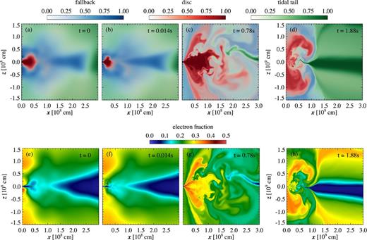
Snapshots in the evolution of the high-resolution 2D model C2d-res, which evolves the entire merger remnant (disc+dynamical ejecta) including the effects of shear viscosity and neutrinos. The upper four panels (a)–(d) show the mass fractions of passive scalars that trace the different components of the system as defined in Section 2.2: disc (red), fallback (blue), and tidal tail (green). The lower four panels (e)–(h) show electron fraction. Note the change in x- and z-scale in panels (d) and (h).
The mass outflow rate as a function of time at a radius of 109 cm is shown in Fig. 3 for models C2d (all components), C2d-df (no tidal tail), C2d-h (radioactive heating), and C2d-res (all components at double resolution in radius and polar angle). The contribution from the disc and fallback scalars is shown as well as the total mass outflow including tidal tail material. At early times, mass ejection is dominated by the tidal tail, transitioning around t ∼ 1 s to dominance by the disc wind. At late times, the instantaneous outflow rate at large radii is not very sensitive to whether the tidal tail is present or not, and whether radioactive heating is included.
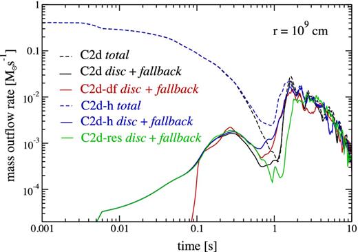
Mass outflow rate at r = 109 cm as a function of time for different 2D models. The total outflow rate, including the tidal tail, is shown by dashed lines. The ‘wind’ (solid lines) includes material that is tagged as disc and fallback in the initial condition, as defined in Section 2.2. The qualitative evolution relative to the baseline model (black) is independent of whether radioactive heating is included (blue), whether the tidal tail is excluded (red), or if the resolution is doubled in radius and polar angle (green).
Table 1 shows integrated properties of the 2D models over 10 s of evolution. The total mass ejected is of the order of 20 per cent of the initial disc mass (∼0.04 M⊙), in agreement with previous results for a BH with spin a = 0.8 (Fernández et al. 2015; Just et al. 2015). The fraction of this outflow that has positive specific energy (with the internal energy normalized so that it vanishes at T = 0) lies between 50 and 60 per cent. The mean velocity of this unbound wind is ∼0.04c. Radioactive heating leads to a ∼15 per cent enhancement in the unbound mass ejection, whereas excluding the tidal tail leads to ∼10 per cent less mass ejected due to the absence of leftover material swept up by the wind. The overall uncertainty due to resolution is ∼10 per cent.
Mean properties of the disc wind in 2D models. Columns are model name, electron fraction, entropy, and expansion time. The mass-flux-weighted, time-averaged quantities are computed using equation (8), at a radius where |$\bar{T}\simeq 5\times 10^9$| K (∼1000–1500 km). Only material tagged as disc and fallback is included.
| Model | |$\bar{Y}_{\rm e}$| | |$\bar{s}$| | |$\bar{t}_{\rm exp}$| |
|---|---|---|---|
| (kB b−1) | (ms) | ||
| C2d | 0.29 | 32 | 66 |
| C2d-df | 0.27 | 29 | 111 |
| C2d-d | 0.28 | 29 | 96 |
| C2d-h | 0.28 | 32 | 83 |
| C2d-res | 0.28 | 33 | 48 |
| C2d-src | 0.27 | 29 | 28 |
| Model | |$\bar{Y}_{\rm e}$| | |$\bar{s}$| | |$\bar{t}_{\rm exp}$| |
|---|---|---|---|
| (kB b−1) | (ms) | ||
| C2d | 0.29 | 32 | 66 |
| C2d-df | 0.27 | 29 | 111 |
| C2d-d | 0.28 | 29 | 96 |
| C2d-h | 0.28 | 32 | 83 |
| C2d-res | 0.28 | 33 | 48 |
| C2d-src | 0.27 | 29 | 28 |
The mean electron fraction of the wind is ∼0.26–0.29, slightly higher than that obtained with a smaller BH mass and more compact discs, starting from an equilibrium initial condition, and using the same neutrino implementation (e.g. Fernández et al. 2015). The mean entropies are ∼30kB per baryon and the expansion time lies in the range 50–100 ms. Given these parameters, the critical electron fraction above which no lanthanides are produced is ∼0.25 (Kasen et al. 2014). The disc wind will therefore lead primarily to lanthanide-free material and a kilonova component peaking in the optical band.
The accretion history at the ISCO is shown in Fig. 4. The initial transient phase is evident, with even a short period during which no accretion takes place. From the end of this transient phase at t ≃ 0.02 s until approximately t = 1 s, the accretion rate evolves smoothly. After the wind is launched, however, the time dependence of the accretion rate steepens, with the asymptotic power law in the range t−2.15 – t−2.3. Such a drop in the accretion rate at late times was first seen by Lee et al. (2009). In the context of fallback accretion, we note that this time dependence is insensitive to whether material labelled as fallback and tidal tail is included, as shown in Fig. 4 (model C2d-d includes only material labelled as disc).

Net mass accretion rate at the ISCO for 2D models (see Table 1 for parameters). The late-time accretion rate is somewhat steeper than that due to ballistic fallback, and is set by the viscously spreading disc. The temporal slope does not significantly depend on whether the dynamical ejecta and fallback are excluded, whether radioactive heating is added, or on the resolution of the simulations. At early times (t ≲ 0.01 s) the disc is undergoing transient readjustment.
Indeed, one can show using simple scaling arguments that during the late radiatively inefficient phase of evolution, the mass accretion rate scales like t−4/3 (Metzger, Piro & Quataert 2008). This scaling becomes even steeper (t−8/3) when outflows are included in the solution. Our models have an intermediate behaviour between these two limits.
3.2 Fallback accretion without disc wind: effect of radioactive heating
Fig. 5(a) shows the mass accretion rate at the inner radial boundary of the 3D computational domain (r = rcut = 800 km) for model F3d, which does not include the effect of the disc wind or radioactive heating, instead simply letting all material evolve under the effects of gravity. The accreted material at r = 800 km is initially composed primarily of fluid tagged as fallback. Around t = 2 s, the composition becomes dominated by tidal tail material. As pointed out in Section 2.2, approximately 0.01 M⊙ of tidal tail material is gravitationally bound due to spatial overlap with other components. This material is almost completely accreted during the simulated time.
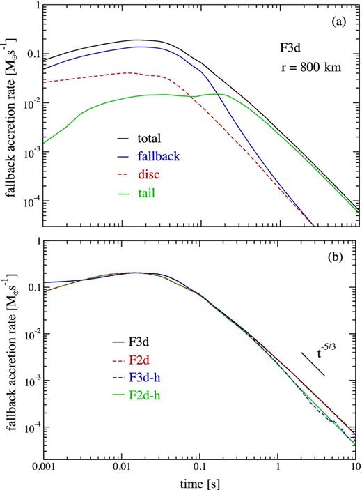
Mass accretion (fallback) rate as a function of time at r = rcut = 800 km for models without wind injection. Panel (a) shows the accretion rate for model F3d, which ignores radioactive heating. Also shown are the contributions from the different components of the system (Section 2.2) as traced by passive scalars. Panel (b) compares 2D and 3D models with and without radioactive heating. While radioactive heating causes a temporary steepening of the accretion rate with time, its overall effect is small. Models in 2D and 3D are very close to each other at late times.
The accretion rate at r = rcut in all models that do not include the disc wind is shown Fig. 5(b). Models F2d and F3d (no radioactive heating) differ slightly in their initial evolution until ∼1 s, after which they display a nearly identical accretion history. The fact that the time dependence of this accretion is very nearly t−5/3 indicates that the mass distribution is close to uniform in orbital energy, and that the contribution from the fluid pressure to the dynamics is minor.
Including radioactive heating modifies the evolution of the accretion rate on the expected time-scales (equation 10) by steepening the time dependence over the interval 0.3–3 s. This is shown in Fig. 5(b), where models F2d-h and F3d-h are shown alongside models that do not include heating. While a gap in the fallback rate, as envisioned by Metzger et al. (2010a), does not appear, the accretion rate is suppressed over a finite interval relative to the case without heating, returning later to the approximate t−5/3 scaling. The absence of a gap can be explained by the constancy of dM/dEorb (equation 9) as inferred from the models without radioactive heating. Addition of energy by the r-process simply shifts mass in this distribution towards higher energies, filling the gap near Eorb = 0 with material that initially had lower energy.
The total accreted material for all models in this sequence lies in the range 0.026–0.029 M⊙. If the accretion rate were to continue indefinitely with the same magnitude and scaling as it has at t = 10 s, only an additional ∼10−4 M⊙ would be added.
3.3 Effect of disc wind on fallback accretion
The disc wind causes important changes in the properties of fallback accretion. This was already seen in the 2D results of Section 3.1, where the disc completely dominates over fallback material in setting the late-time accretion rate (Fig. 4). Here we examine this interplay using more realistic 3D simulations, in which the wind measured in 2D models is injected from the inner radial boundary at r = rcut = 800 km. Fig. 6(a) compares the evolution of the mass accretion rate in our 3D simulations with and without wind. We isolate material that is initially outside r = rcut by assigning a passive scalar Xinj = 1 to all material that is subsequently injected into the domain, independent of which component of the system (Section 2.2) it is made of. We then compute the total mass flux with negative radial velocity at the inner boundary, multiply by (1 − Xinj), and integrate in solid angle. Fig. 6 shows that fallback accretion is suppressed after t ∼ 100 ms when the wind is injected.
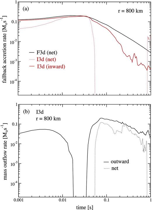
Panel (a): accretion rate at r = rcut = 800 km in models that evolve the dynamical ejecta in 3D with wind injection (I3d) and without wind (F3d). The curve labelled ‘inward’ includes only material initially present in the domain and with negative radial velocity at the inner boundary, for comparison with the model without wind. The net accretion rate for model I3d includes all material. Panel (b): mass outflow rate in the fiducial model I3d. Shown are the total amount of material with positive velocity injected into the domain (‘outward’) and the net outflow rate including all material. The first outflow episode (t < 0.02 s) corresponds to dynamical ejecta material moving outward, with the second caused by the disc wind (cf. Fig. 3).
Small quantitative modifications in the evolution of the accretion rate around and after the onset of the wind are obtained when including radioactive heating, when using a different treatment for the wind injection, and when using the wind from model C2d-df, which does not include the feedback from the tidal tail in 2D (cf. Table 1).
The net accretion rate (all material) at r = rcut for the fiducial model is also shown in Fig. 6(a). Initially, this net accretion rate is lower than the case with no wind injection. This decrease is caused by dynamical ejecta material moving outward, as shown in Fig. 6(b). Once this initial outflow subsides, the net accretion rate reaches its full magnitude around t ∼ 30 ms. Shortly thereafter, the net accretion rate becomes net outflow once the wind turns on.
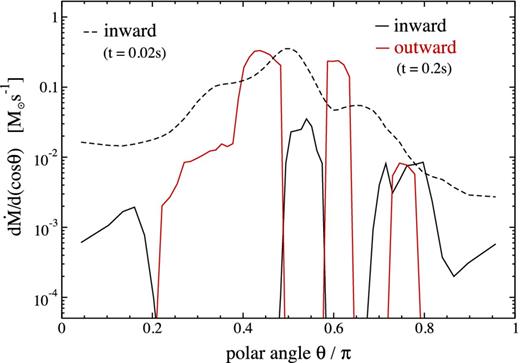
Distribution of the mass flow rate at r = rcut as a function of polar angle (equation 11) for the fiducial 3D model with wind injection (I3d) at two times. The inward accretion rate includes only material initially present in the domain and which has negative radial velocity at the inner radial boundary. The outflow rate includes only material injected into the domain. Compare with Fig. 6.
At about t ∼ 1 s, our diagnostic for the inflow at r = rcut shows that net accretion resumes, with strong stochastic fluctuations (Fig. 6 a). This is, however, related to the spreading of the accretion disc outside r = 800 km. In other words, the outer edge of the radiatively inefficient, convective accretion disc enters the 3D computational domain, with the wind-launching radius moving continuously outward.1
3.4 Properties of the disc wind and dynamical ejecta at large radii
By the end of our simulations, at t = 10 s, the system is approaching homology: the material outside r ≃ 2 × 1010 cm has radial velocity roughly proportional to radius (∼r0.95). This material amounts to 60 per cent of the mass in the computational domain.
The geometry of these homologous ejecta is shown in Fig. 8. The tidal tail wraps around the rotation axis, occupying primarily the equatorial plane. The wind is located at the centre of the domain, expanding towards high to intermediate latitudes. Because the wind is expanding more slowly than the dynamical ejecta by a factor of several, in the homologous limit its spatial extent must be smaller by the same factor.

Isosurfaces of passive scalars tracing material initially tagged as tidal tail (90 per cent mass fraction, green) and wind (disc+fallback) (5 and 95 per cent mass fraction, blue and red, respectively) at time t = 10 s. Shown are the fiducial 3D model of dynamical ejecta evolution with disc wind injection from the inner boundary (I3d, left) and a version that adds radioactive heating by the r-process (I3d-h, right). Most of the material shown is already in homologous expansion, hence its geometry will not change at later times.
Including radioactive heating smoothes inhomogeneities in the tidal tail, increasing its vertical extent due to the added thermal energy, as shown in Fig. 8. This result is consistent with the findings of Rosswog et al. (2014). In terms of the expected electromagnetic counterpart, this implies that neutron-rich (and hence high optical opacity) material in the tidal tail obscures the disc wind component for a larger set of viewing angles along the equator (e.g. Kasen et al. 2014), relative to the case without radioactive heating. Given this particular set of initial conditions, however, the tidal tail does not cover all azimuthal angles, hence the expected optical emission from the disc wind can readily escape along those unobstructed viewing directions.
The material in the tidal tail is significantly more neutron rich than that in the disc wind, as is well known. Fig. 9 shows slices of the electron fraction distribution normal to the x and z axes, illustrating the spatial distribution of material that will give rise to lanthanide-rich (Ye ≲ 0.25) and lanthanide-poor ejecta (Ye ≳ 0.25; see e.g. Kasen et al. 2014). Fig. 10 shows a mass histogram as a function of electron fraction for models I3d and I3d-h, including all material crossing a surface at r = 3 × 109 cm. The histograms are bimodal, with clear contributions from the tidal tail at Ye ≲ 0.05, and disc wind at Ye ∼ 0.25. At small amount of tidal tail material is mixed with the wind, and has higher electron fraction.
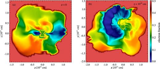
Electron fraction in the fiducial 3D model I3d at time t = 10 s. Shown are 2D slices normal to the x-axis (a) and normal to the z-axis (b). Compare with Fig. 8.

Mass histograms as a function of electron fraction for models I3d and I3d-h (cf. Fig. 9). The histograms are computed by summing all the material crossing the radius r = 3 × 109 cm over the entire simulation time (t = 10 s).
Our method of injecting the wind from the inner radial boundary works well as long as the disc does not enter the computational domain. Once the disc enters, around t ∼ 1 s, there is a discrepancy between the stresses at this boundary and those that would be obtained in a self-consistent simulation. In particular, the use of an outflow boundary condition whenever the radial velocity at the boundary is negative leads on average to lower pressure support on the section of the disc that has entered the domain.
The consequence of this discrepancy in stresses is a decrease in the amount of mass ejected to large radius in models with wind injection relative to a self-consistent simulation. Table 1 shows that this discrepancy is a factor of ∼2, and is independent of whether 2D or 3D is employed (model I2d versus C2d) or whether neutrino and viscous source terms are included in the self-consistent model (models C2d versus C2d-src).
We can nevertheless still compare the bulk properties of the wind at large radius between 3D models, using the 2D model with wind injection (I2d) as a baseline. Table 1 shows that the specific wind injection method (solving a Riemann problem or simply filling the ghost cells with the sampled wind) is largely unimportant in determining the wind properties at a radius r = 109 cm. Including radioactive heating does indeed lead to more mass ejection, with an enhancement similar to that observed in the 2D models. Similarly, injecting the wind sampled from model C2d-d (no tidal tail) leads to correspondingly small mass ejection.
The velocity and electron fraction of the wind undergo small changes relative to 2D. While both increase relative to the 2D models, the change is not likely to lead to qualitative differences in their nucleosynthetic properties and in their effect on the observed kilonova. In the case of the electron fraction, this implies that there is no significant mixing between wind material and the bulk of the dynamical ejecta, which would otherwise have lowered Ye from its pure wind value. While Fig. 8 indicates that some mixing does indeed occur in the immediate vicinity of the wind, the amount of mass affected is a small fraction of the total, and goes in the direction of making tidal tail material more proton rich (Fig. 10). This low degree of mixing is a consequence of the factor of 2–4 faster radial velocity of the dynamical ejecta.
4 SUMMARY AND DISCUSSION
We have investigated the interaction between the disc wind and dynamical ejecta generated in an NS–BH merger. Starting from the output of a Newtonian merger simulation, we have disentangled the ejecta components using its phase-space distribution (Section 2.2). The disc is located at small radii and is nearly axisymmetric, hence the resulting disc wind can be estimated from axisymmetric simulations to first approximation. Given that viscous and neutrino source terms are subdominant in the outer regions of the system, where the non-axisymmetric dynamical ejecta resides, one can evolve this component in 3D without the high computational cost of viscous or neutrino processes. We therefore inject the axisymmetric disc wind from the inner boundary of the 3D computational domain.
By following this two-step approach, we obtain the following results.
Fallback accretion can be suppressed once the disc wind is launched (Fig. 6). In our models, this happens ∼100 ms into the simulation.
The properties of the disc wind are not significantly affected by the dynamical ejecta. This is largely due to the difference in expansion velocities. Most of the gravitationally bound part of the dynamical ejecta (‘fallback’, Section 2.2) is swept up by the wind, forming its leading edge (Fig. 2d). While some small amount of mixing occurs between material coming from the disc and that in the tidal tail, it goes primarily in the direction of making tidal tail material more proton rich (Fig. 10).
The time dependence of the mass accretion rate at the ISCO steepens after the wind is launched. For our choice of parameters, it follows a slope ∼t−2.2 (Fig. 4). This is nearly independent of whether the tidal tail and fallback components are included in the simulation. This power-law decline is set by the physics of the viscously spreading disc with outflows (Metzger et al. 2008), not fallback.
We do not find a gap in the fallback accretion rate induced by radioactive heating when the wind is ignored (Fig. 5). Instead, we find a steepening in the time dependence of this accretion rate over a finite interval, resuming the quasi-ballistic t−5/3 time dependence at late times. Inclusion of radioactive heating in disc wind simulations yields a small (∼10 per cent) enhancement in the ejected mass (Table 1), with no qualitative differences in the ejecta composition (Table 2).
We find that including radioactive heating smoothes out inhomogeneities in the tidal tail (Fig. 8), in agreement with Rosswog et al. (2014). This results in very neutron-rich material (with high optical opacity) obscuring a larger fraction of the available viewing directions towards the wind ejecta, which has a smaller size in the homologous limit due to its smaller velocity. However, the specific model we evolved is such that the tidal tail does not cover all azimuthal angles (Fig. 9), leaving a wide range of unobstructed sight lines.
The properties of the disc outflow are qualitatively similar to those obtained from simulations with spinning BHs that begin from idealized initial conditions with somewhat less massive and more compact discs (e.g. Fernández et al. 2015).
While our quantitative results are specific to the particular initial condition we have adopted, our approach contains several features that can be useful in future studies of the interplay between the different components of the combined merger ejecta. First, we have found a novel way to isolate the dynamical ejecta – bound and unbound gravitationally – from rotationally supported material. Secondly, we have shown that ignoring neutrino and viscous source terms at large radii (r ≳ 108 cm) has a minor effect on the evolution of the system. The main drawback of our method is the treatment of the boundary condition when the radial velocity is negative. At times t ≳ 1 s, the disc has spread out sufficiently to enter our 3D domain. If the stresses ensuing from this boundary condition are not sufficient to support the part of the disc inside the domain, an excess of mass will flow inwards, significantly affecting the amount of wind launched to large radii. Large-domain axisymmetric simulations are a reasonable way to improve this analysis, given the similarity in the globally integrated properties.
The fact that we have found no significant mixing between the disc wind and dynamical ejecta means that separately estimating the nucleosynthetic contribution from the disc and tidal tail is a reasonable approximation. This is relevant given that the two components are expected to lead to different nucleosynthetic signatures, with implications for the dispersion in the r-process abundance in the galaxy (Just et al. 2015) and the properties of the kilonova emission (Kasen et al. 2014; Metzger & Fernández 2014).
Even though our results show that fallback accretion is not always a robust source of late-time engine activity in short GRBs, the fact that accretion from the disc continues for a long time provides a persistent source of accretion power. However, the steeper decline with time in the accretion rate relative to ballistic fallback (t−2.2 versus t−5/3) implies that after 104 s, the energy output from accretion is ∼30 times smaller (disc accretion is ∼3 times larger than wind-free fallback at t = 1 s, cf. Figs 4 and 5). This is illustrated in Fig. 11, which shows the extrapolation of the mass accretion rate at the ISCO for the default 2D model C2d, together with the extrapolation of the fallback accretion rate (without the effect of the disc wind) at r = 800 km from model F3d. The extrapolation of the fallback rate is an upper limit, however, given that material has angular momentum and may circularize at a radius larger than the ISCO. In this case, material will contribute to whatever remains of the disc and accretion will proceed at a rate set by viscous processes, eventually acquiring a t−2.2 time dependence. Even if fallback material has low angular momentum, the presence of the disc will prevent it from falling directly on to the BH, particularly along the midplane.
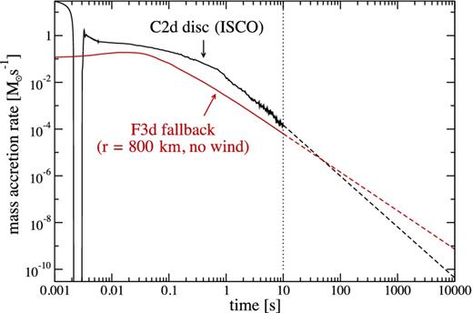
Extrapolation of the mass accretion rate from disc accretion at the ISCO (black, model C2d) and fallback with no wind at r = 800 km (red, model F3d) after t = 10 s, illustrating the smaller energy released by the disc at times where extended GRB central engine emission and/or X-ray flares takes place.
If accretion indeed dominates late-time engine activity, time variability can result if instabilities occur in the outer disc (Perna, Armitage & Zhang 2006) or near the BH due to magnetic effects (Proga & Zhang 2006). Even if accretion is smooth, late-time variability can result if the surrounding medium is excavated by Poynting flux if the NS is a pulsar before the merger (Holcomb et al. 2014).
The observed suppression of fallback in our models is contingent on the initial condition we have chosen to carry out our study, and hence it is not necessarily a general property of NS–NS or NS–BH mergers. In our simulations, the amount of mass ejection in the wind (0.04 M⊙, or ∼20 per cent of the initial disc mass) is larger than the initial amount of fallback and bound tidal tail material (0.03 M⊙). Inclusion of GR and a slightly different set of binary parameters (including eccentricity; East, Pretorius & Stephens 2012) can in principle lead to a different hierarchy. For example, Foucart et al. (2014) find disc masses in the range 0.04–0.14 M⊙ and bound dynamical ejecta in the range 0.03–0.05 when considering mergers of NSs with 7 M⊙ BHs in GR. Their lowest disc mass is a factor of 5 smaller than ours, and the expected fallback is a factor of ∼2 larger. In this case, does the disc wind escape at intermediate latitudes while fallback proceeds and keeps the mass supply constant? Or does fallback suppress the onset of the wind, entraining material back to the disc?
In the case of NS–NS mergers, the dynamical ejecta is less concentrated in the midplane than in BH–NS mergers of large mass ratio (e.g. Bauswein et al. 2013; Hotokezaka et al. 2013). For similar relative masses between bound dynamical ejecta and disc, the more spherical geometry should make it easier for the disc wind to disrupt fallback.
Our calculations can be improved in many ways. Injection of the wind into an expanding boundary in 3D models would alleviate the problems introduced when the disc enters the domain, and allow a better estimate of the degree of mixing between tidal tail and disc. The wind calculations can be made more realistic by including magnetohydrodynamics (MHD) and GR effects self-consistently. The composition of the wind can be better quantified by using an improved neutrino transport scheme. The contribution of radioactive heating to the dynamics of fallback material can be studied further by accounting for the increase in temperature of fluid elements as they fall towards the BH (the prescription we employed assumes that all fluid elements are in continuous expansion, thus overestimating the energy release). Future studies will address these improvements.
We thank Brian Metzger, Frank Timmes, and the anonymous referee for constructive comments that improved the paper. RF acknowledges support from the University of California Office of the President, and from NSF grant AST-1206097. EQ was supported by NSF grant AST-1206097, the David and Lucile Packard Foundation, and a Simons Investigator Award from the Simons Foundation. JS is supported by the National Science Foundation Graduate Research Fellowship Program under Grant No. DGE 1106400. DK was supported in part by a Department of Energy Office of Nuclear Physics Early Career Award, and by the Director, Office of Energy Research, Office of High Energy and Nuclear Physics, Divisions of Nuclear Physics, of the US Department of Energy under Contract No. DE-AC02-05CH11231. SR was supported by the Deutsche Forschungsgemeinschaft (DFG) under grant RO-3399, AOBJ-584282 and by the Swedish Research Council (VR) under grant 621-2012-4870. The software used in this work was in part developed by the DOE NNSA-ASC OASCR Flash Center at the University of Chicago. This research used resources of the National Energy Research Scientific Computing Center (NERSC), which is supported by the Office of Science of the US Department of Energy under Contract No. DE-AC02-05CH11231. Computations were performed at Carver and Hopper (repos m1186, m1896, and m2058).
While the position of the outer edge of the disc is not uniquely defined, we estimate it by computing an isodensity surface at 10−4 times the instantaneous density maximum.
