


Abstract
New high-resolution spectroscopy and BVR photometry, together with literature data, on the Gould's Belt close binary systems GG Lup and μ1 Sco are presented and analysed. In the case of GG Lup, light and radial velocity curve fittings confirm a near-main-sequence picture of a pair of close stars. Absolute parameters are found, to within a few per cent, thus: M1 = 4.16 ± 0.12, M2 = 2.64 ± 0.12 (M⊙); R1 = 2.42 ± 0.05, R2 = 1.79 ± 0.04 (R⊙); T1 ∼ 13 000, T2 ∼ 10 600 (K); photometric distance ∼160 (pc). The high eccentricity and relatively short period (105 yr) of apsidal revolution may be related to an apparent ‘slow B-type pulsator’ oscillation. Disturbances of the outer envelope of at least one of the components then compromise comparisons to standard evolutionary models, at least regarding the age of the system. A rate of apsidal advance is derived, which allows a check on the mean internal structure constant |$\overline{k_2} = 0.0058 \pm 0.0004$|. This is in agreement with values recently derived for young stars of solar composition and mass ∼3 M⊙. For μ1 Sco, we agree with previous authors that the secondary component is considerably oversized for its mass, implying binary (interactive) stellar evolution, probably of the ‘Case A’ type. The primary appears relatively little affected by this evolution, however. Its parameters show consistency with a star of its derived mass at age about 13 Myr, consistent with the star's membership of the Sco–Cen OB2 Association. The absolute parameters are as follows: M1 = 8.3 ± 1.0, M2 = 4.6 ± 1.0 (M⊙); R1 = 3.9 ± 0.3, R2 = 4.6 ± 0.4 (R⊙); T1 ∼ 24 000, T2 ∼ 17 000 (K); photometric distance ∼135 (pc).
1 INTRODUCTION
Our work on young southern binary systems has been presented in several earlier papers concentrating on individual well-documented examples. In this paper we consider two close binaries – GG Lup and μ1 Sco – that allow more compact summaries. Further background was given by Budding (2008 – hereafter ‘Paper I’). A recent general review was given by Idaczyk et al. (2013). The Andersen (1991) review gave an interesting rationale for this kind of work.
We give more particulars on GG Lup next. Photometric data (Section 2.1) are later combined with new spectroscopic material (Sections 2-2– 2.5) to refine knowledge of the absolute parameters of the components (Section 2.6). A similar treatment then follows for μ1 Sco in Section 3. Section 4 summarizes the derived information on both binaries within the context of their Galactic environment. This arrangement follows similar lines to that of previous papers of this programme.
Although these two young, short-period, early-type systems are both likely members of the Sco–Cen OB2 Association and of comparable age, their physical characteristics are quite different in some respects. They do, however, both show indications of additional variability, beyond that associated with close binarity. Such effects compromise their precise parametrization. We aim to clarify the background on their observed properties. At the same time, we challenge some of the claims of previous authors on modelling details.
2 GG Lup
GG Lup (= HD 135876, HIP 74950, HR 5687) is a relatively bright (V ∼ 5.5–6.1, B − V ≈ −0.099, U − B ≈ −0.46, V − I ≈ −0.08, V − J ≈ −0.530, V − H ≈ −0.667, V − K ≈ −0.625; Cutri et al. 2003), young B7V + B9V type close binary system with period P ≈ 1.85 d, having a known appreciable eccentricity e ≈ 0.15. Neubauer (1930) discovered it as a close spectroscopic pair. Photometry showing eclipses later appeared from Smith (1966) and Strohmeier (1967). A thorough study was given by Andersen, Clausen & Giménez (1993) who, noting the youth of the stars (age estimated at ∼20 Myr), found a relatively short period of just over 100 yr for its apsidal advance. This was confirmed by Wolf & Zejda (2005), although the coverage of the O − C curve is still not great.
The sky location RA (2000) = 15h18m56s, Dec. (2000) = −40°47′18″, HIPPARCOS distance 162 ± 17 pc and proper motions (μαcos δ ≈ −24, μδ ≈ −22 mas yr−1) make the system a likely member of the Upper Centaurus Lupus (UCL) concentration (Blaauw 1964) of the Sco–Cen OB2 Association, within the Gould's Belt giant star formation region (Nitschelm 2004). The system lies towards that part of the Belt that is more separated from the Disc (l = 330.9; b = 14.0 deg). The relatively scant attention given previously to this interesting object may be due to its southerly declination (∼ −40 deg).
Wolf & Kern (1983) obtained uvbyβ measures for GG Lup, noting a need for a revised ephemeris, while Levato & Malaroda (1970), at La Plata Observatory, published a fairly high projected rotational velocity of 155 km s−1, presumably of the primary component. Andersen et al. (1993) emphasized the implications of their parameters for the system on the relationship of stellar properties to galactic environment: an issue that has significance to problems of stellar formation in general and Gould's Belt in particular.
2.1 Photometry and analysis
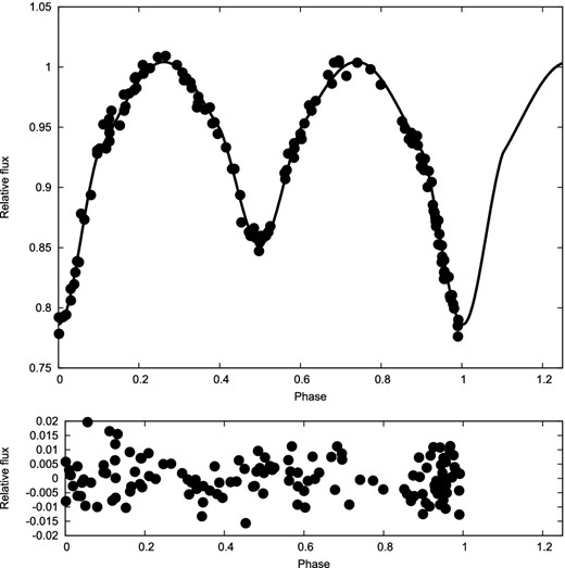
We start with an examination of the HIPPARCOS light curve (ESA 1997). The HIPPARCOS data source gives the ephemeris Min I = 2448 500.55 + 1.849 62E, which can be compared with that of Andersen et al. (1993) Min I = 2446 136.7398 + 1.849 60E. Kreiner, Kim & Nha (2001) refine the ephemeris to Min I = 2446 136.7477 + 1.849 5927E. We show the HIPPARCOS light curve in Fig. 1 together with our best-fitting model, whose main parameters are listed in Table 1. This modelling was done using the program fitter, whose theoretical basis was discussed by Budding & Demircan (2007, chapter 9). The program's operation (recently upgraded to winfitter) has been detailed by Rhodes (2014), while Rhodes & Budding (2014) presented a detailed discussion of the modelling and fitting procedure. The approach uses a standard Marquardt–Levenberg-type optimization technique with a fitting function that derives from the Kopal (1959) linearization of close binary proximity effects in terms of spherical harmonics. The tidal and rotational distortions thus include the effects of finite mass of the envelopes. The reflection terms provide an ‘albedo’ factor (usually unity for radiative envelopes), for possible empirical modification of the luminous efficiency coefficients of Hosokawa (1958).

HIPPARCOS V photometry of GG Lup: model fitting and residuals (see Section 2 for details).

Curve-fitting results for HIPPARCOS photometry of GG Lup. Parameters for which no error estimate is given are adopted from information separate to the fitting.
| Parameter | Value | Error |
|---|---|---|
| Th (K) | 12 000 | |
| Tc (K) | 10 000 | |
| M2/M1 | 0.62 | |
| L1 | 0.79 | 0.01 |
| L2 | 0.21 | 0.01 |
| r1 (mean) | 0.204 | 0.003 |
| r2 (mean) | 0.141 | 0.004 |
| i (deg) | 88.3 | 1.4 |
| e | 0.15 | |
| ω | 108.1 | 0.4 |
| u1 | 0.35 | |
| u2 | 0.41 | |
| Δϕ0(deg) | −2.07 | |
| χ2/ν | 1.05 | |
| Δl | 0.007 |
The mean epoch of the HIPPARCOS observations is given as HJD 2448349.0625, almost six months before the time of minimum given above, and the data was collected over an approximately 3 yr interval, so some uncertainty in the timing of the relevant periastron longitude arises. A more representative average epoch for the HIPPARCOS data would be HJD 2448348.881; some 82 periods before the cited one.
Turning to the uvby data of Clausen et al. (1993) as cited by Andersen et al. (1993), we provide the results of curve-fitting experiments in Table 2, with corresponding diagrams in Figs 2 and 3. Table 3 provides the adopted reference mean magnitudes, in various filter regions, using fittings for the relative luminosities as shown in Table 2. Andersen et al. (1993) gave a value of 0.006 mag as a representative error for their photometry. With the added uncertainties of the fittings and the non-uniformity of the magnitude scale this translates to ∼0.01 mag for the brighter component and 0.05 mag for the fainter star.
Curve-fitting parameters for the Clausen et al (1993) uvby photometry of GG Lup. Error estimates are shown by the bracketed numbers, that relate to the final digit of the parameter values. Otherwise, parameter valued are adopted.
| Parameter | Value | ||||
|---|---|---|---|---|---|
| mean | u | v | b | y | |
| Th (K) | 12 000 | ||||
| Tc (K) | 10 000 | ||||
| M2/M1 | 0.62 | ||||
| L1 | 0.841(7) | 0.776(6) | 0.755(6) | 0.747(6) | |
| L2 | 0.159(5) | 0.224(4) | 0.245(4) | 0.253(4) | |
| r1 | 0.201(1) | ||||
| r2 | 0.149(1) | ||||
| i (deg) | 87.5(4) | ||||
| e | 0.154 | ||||
| ω (deg) | 86.3(1) | ||||
| u1 | 0.43 | 0.43 | 0.40 | 0.35 | |
| u2 | 0.46 | 0.50 | 0.47 | 0.41 | |
| Δϕ0(deg) | 1.63 | ||||
| χ2/ν | 1.13 | ||||
| Δl | 0.0025 | ||||
Magnitudes of stars in the GG Lup system. Errors are discussed in Section 2.1.
| u | v | B | b | |
| msys | 6.194 | 5.612 | 5.549 | 5.547 |
| m1 | 6.382 | 5.887 | 5.733 | 5.852 |
| m2 | 8.19 | 7.24 | 7.09 | 7.07 |
| y | VH | V | R | |
| msys | 5.589 | 5.577 | 5.558 | 5.613 |
| m1 | 5.906 | 5.847 | 5.853 | 5.911 |
| m2 | 7.08 | 7.22 | 7.12 | 7.16 |
| u | v | B | b | |
| msys | 6.194 | 5.612 | 5.549 | 5.547 |
| m1 | 6.382 | 5.887 | 5.733 | 5.852 |
| m2 | 8.19 | 7.24 | 7.09 | 7.07 |
| y | VH | V | R | |
| msys | 5.589 | 5.577 | 5.558 | 5.613 |
| m1 | 5.906 | 5.847 | 5.853 | 5.911 |
| m2 | 7.08 | 7.22 | 7.12 | 7.16 |
2.1.1 Oscillatory effects
Andersen et al. (1993) referred to systematic out-of-eclipse variations, visible in the enlarged scale of Fig. 3, as residual inherent variation of the source that could not be removed by eclipsing binary model parameter adjustments. They mentioned forced oscillations, tidal lag or non-aligned rotation axes as possible causes. They did not pursue such effects, however, concentrating their study on the determination of basic stellar absolute parameters. Tidal lag or non-aligned rotation axes can be seen as somewhat particular examples of general dynamical effects for the fluid masses making up this close pair (probably not very effective, taken individually, in accounting for the scale and apparent periodicity of the effects).
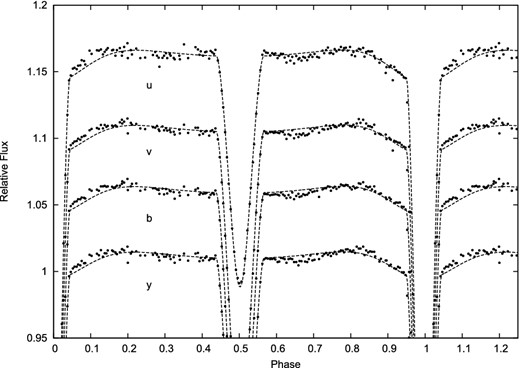
uvby photometry with enlarged ordinate scale, showing the oscillatory behaviour mentioned by Andersen et al. (1993).
We may thus consider the apparent three-to-one resonance between the oscillatory and orbital photometric variations within the context of forced effects associated with the unusually high eccentricity of the system and some inherent overstability of at least one of the component stars. Lampens (2006), noting the special relevance of young star associations in this context, considered the sequence of interactions involving orbital motion, rotation and pulsation as an interesting question, still open to detailed study. An interesting review on this subject was given by Harmanec et al. (1997), as an introduction to their concentrated work on the comparable, but much longer period eclipsing binary system V436 Per. The Chapellier et al. (1995) study of the early-type eccentric eclipsing binary EN Lac is also noteworthy in this context. Orbital circularization in early-type close binaries is expected to be a relatively fast process (Zahn 1977), i.e. τcirc < 106 yr, in general. This process would probably involve dissipative mechanisms related to g-mode oscillations (Henrard 1982; Alexander 1987, 1988; Witte & Savonije 1999).
If there already exists a κ-mechanism capable of generating inherent non-radial pulsations, particular arrangements of the eccentricity that would otherwise produce the same or similar modes may become trapped, since the dissipation affecting such modes would, in this case, be accounted for by the κ-mechanism. Work otherwise drawn from the reserve of orbital energy to cover dissipation of the excited fluid motions now comes from another source and the corresponding secular decline of eccentricity halted. Such motions are, from an idealized classical mechanics point of view, as capable of putting energy back into the orbit as being stimulated by that. But the configurations that would be more likely observed would be the quasi-static ones, where the oscillation driving just matches secular dissipation. Relative minima of the net disturbing potential would then be expected, out of which the orbit would be gradually perturbed by evolutionary changes of the κ-mechanism. In the case of slow B-type pulsator (SPB) oscillations, these can be expected over the star's main-sequence lifetime. But Lampens (2006) notes, pointedly, that six of the seven short-period SPBs found in close binary systems by De Cat & Aerts (2002) were in eccentric orbits.
The criteria discussed by De Cat & Aerts (2002) for establishing the SPB nature of a star usually involve at least two separate photometric samplings together with spectroscopic evidence, and one of the photometric sources they refer to is HIPPARCOS. In our present case, however, the amplitude of the photometric oscillation appears relatively small at ∼0.005 mag, and this is appreciably below the scatter of residuals (∼0.01 mag) in the HIPPARCOS light curve. We were therefore interested to check the photometric indications shown by Andersen et al. (1993) by an alternative technique and the application of a modern digital single-lens reflex (DSLR), high pixel count camera to this (Blackford & Schrader 2011) was opportune.
2.1.2 New photometry
Times of minima and BVR photometry of GG Lup and other stars have been conducted under the Southern Eclipsing Binaries Programme of the Variable Stars South (VSS) section of the Royal Astronomical Society of New Zealand (RASNZ). The GG Lup data were gathered using an unmodified Canon 450D (Digital Rebel XSi) and Nikkor 180 mm lens operated at f4. An unmodified Canon 600D (Digital Rebel T3i) and Canon 200 mm lens operated at f4 were used to collect similar data more recently.
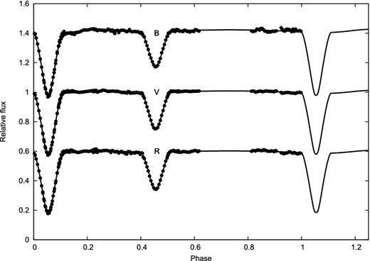
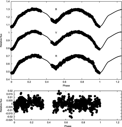
The Bayer filter array employed in DSLR cameras allows simultaneous recording of three colour (rgb) images, from which separate single colour images can be extracted and calibrated. From these images the instrumental magnitudes are determined by differential aperture photometry using an ensemble of comparison stars (six for GG Lup). Atmospheric extinction correction was performed and instrumental magnitudes transformed to the standard (Johnson BVR) system. Our GG Lup light curves are shown in Fig. 4, where we also show optimal fits to the reduced B, V and R data sets.
DSLR photometry of GG Lup and model fitting. Residuals are shown in Fig. 6.
The V residuals were subject to a frequency analysis using purpose-built (python) software carrying out a Lomb–Scargle and the results displayed in Figs 5 and 6. Apart from any indications of additional oscillatory behaviour that the eye can detect in the upper panels of these diagrams, the lower parts confirms the quasi-resonant P/3 character in the residual variations of the Clausen et al. (1993) data (Fig. 5), and is suggestive, though not strongly corroborative, of such behaviour in our own more recent data (Fig. 6).
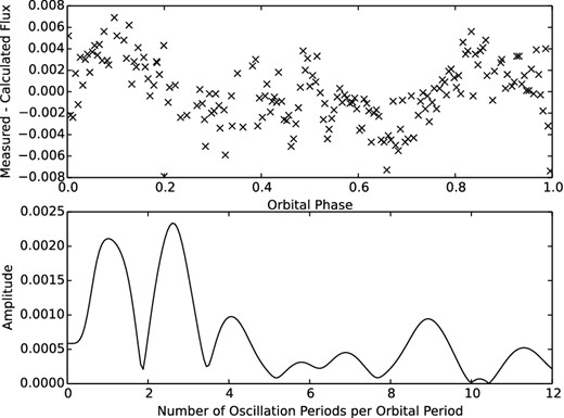
The Andersen et al. (1993) y residuals, with periodicity analysis shown in the lower panel.

The effects of orbital eccentricity are clear in the light curves shown in Figs 1–4. Those produced around 1985 (Clausen et al. 1993) or 1991 (HIPPARCOS) show the secondary minimum occurring about half-way between the primary minima, though they are distinctly wider. The line of apses must then be close to the line of sight. The recent DSLR data shown in Fig. 4, on the other hand, show the separation between primary and the following secondary minimum (of very similar widths) to be significantly less than that between secondary and following primary. This implies the line of apses now lying towards perpendicular to the line of sight. The elliptic orbit of the binary must then have rotated by about one-quarter of a complete cycle in the years between the earlier and more recent light curves. The details of the longitude of periastron variation are given in Table 4. The derived mean rate of apsidal advance should not have the same precision as that corresponding to many individual timings of minima, of course; even so, the fittings of a complete light curve, when gathered over a relatively short time, allows the periastron longitude to be accurately determined. Our best estimate for the rate of apsidal advance (one revolution in 106 ± 2 yr) is not so far from the Andersen et al. (1993) value of 101 ± 4 yr, which was matched by Wolf & Zejda (2005), who found 101.6 ± 1 yr, essentially defined by a small number of photoelectric minimum timings over a ∼10 yr interval.
Apsidal advance from the light-curve fittings (Clausen et al. 1993; HIPPARCOS and this study).
| Epoch | ω |
|---|---|
| JD 244 0000 + | (±) |
| 6136.7398 | 86.3(1) |
| 8348.881 | 108.1(4) |
| 160 69.189 | 178.7(1) |
| Epoch | ω |
|---|---|
| JD 244 0000 + | (±) |
| 6136.7398 | 86.3(1) |
| 8348.881 | 108.1(4) |
| 160 69.189 | 178.7(1) |
The implications of the derived rate of apsidal advance on the internal structure of the component stars may be checked following well-known procedures (cf. e.g. Budding 1974). The observed rate of apsidal advance has first to be corrected for a relativistic effect which, using the parameters of Table 7, amounts to some 8.16 per cent of the ratio of the orbital to proper apsidal periods P/U = 4.525×10⁻⁵. Using also the geometrical parameters of Table 2 and the rotation speeds discussed in Section 2.5, together with the formulae in section 4 of Budding (1974), we can derive a value for the mean structural constant (for the two stars) of |$\overline{k_2}$| = 0.0058 ± 0.0004, which compares favourably with the theoretical value of 0.0056 calculated by İnlek & Budding (2012) for a young star of 3 M⊙ and near solar composition; cf. also Claret & Giménez (2010), who give further background on this subject. The independent calculations of İnlek & Budding (2012) for |$\overline{k_2}$| are generally within ∼10 per cent of those of Claret & Giménez (2010) for comparable stellar models. Although our value for |$\overline{k_2}$| is within Claret & Giménez’ (2010) error limit for their theoretical value, it is outside the Andersen et al. (1993) error limit for their own empirical determination.
2.2 Spectroscopy
As in previous similar work (Paper I; Budding, Butland & Blackford 2013) our spectroscopic data were gathered using the High Efficiency and Resolution Canterbury University Large Échelle Spectrograph (HERCULES) of the Department of Physics and Astronomy, University of Canterbury, New Zealand (Hearnshaw et al. 2002). This was used with the 1-m McLellan telescope at the Mt John University Observatory (MJUO) near Lake Tekapo (∼43°59′S, 174°27′E). Some 35 spectra were taken over the period 2006 May 14–19, in fairly clear weather (occasional clouds). The 50-μm optical fibre was mostly used, enabling a resolution of ∼70 000. The CCD (SITe) camera was in position 2 (Skuljan 2004). Typical exposure times were about 500 s. The data have been reduced using the software hrsp version 5 (Skuljan 2012, private communication) that produces output conveniently in fits formatted files.
About 40 clear orders could then be displayed and studied using the program library of iraf. One of the iraf subroutines (splot), for example, allows image statistics to be checked. We could determine in this way a signal to noise ratio (S/N) for continuum pixel regions (away from flaws or telluric effects) to be usually of order 100 (with a ∼10 per cent deterioration from orders 85 to 121: the orders examined in this study). Lines that could be measured well (see Table 5) have a depth of typically 10 per cent of the continuum and a width at base of up to ∼7 Å or ∼250 pixels. The positioning of a well-formed symmetrical line can thus be expected to be typically achieved to within a few pixels or (equivalently) several km s−1. This agrees with the scatter in derived radial velocities (rvs) given below.
iraf also allows the equivalent width (ew) of features to be directly read from splot's profile-fitting tool (‘k’). We could check, in this way, the spectral-type assignations accepted in the literature (although often carried out with different techniques, dispersions and using different features than those available to us). Measured ratios of the H β/He i 6678 ews were typically ∼30. This compares favourably with a mean spectral-type of B8, using the classical guides (e.g. Jaschek & Jaschek 1987) in combination with the synthetic spectra of Gummersbach & Kaufer (2014). It follows that the secondary must be lower in spectral type than the primary, from comparing the relative He i 6678 ews of primary and secondary ∼1.8, given that the continuum luminosity ratio is ∼3 in this part of the spectrum, although the implied difference cannot be greater than two spectral classes.
The reduced high-dispersion data were manipulated as numerical text files, so that individual lines could be fitted with standard ‘dish-shaped’ profiles (convolved with a Gaussian broadening) and the rv determined from the profile centroids. Useful results were obtained from the selection of lines listed in Table 5, particularly the He i lines. Identifiable spectral lines for GG Lup are similar to those listed in Paper I. Certain secondary lines that are normally too weak to measure reliably became relatively strong during the primary minimum phases (e.g. Fe ii 5041.074). Our profile fitting software package (spectrum) was used to derive line-related parameters for the component stars. spectrum, a python module, uses functions from scipy to display spectral lines and fit various user-defined functions to the measured data. In particular, from scipy.optimize the ‘curve_fit’ function, applying non-linear least-squares optimization principles, is used for the fitting as it is tolerant of noisy data.
Spectral lines of GG Lup which were used for rv determination.
| Species | Order no. | Wavelength | Comment |
|---|---|---|---|
| He i | 85 | 6678.149 | strong, p, usable s |
| Si ii | 89 | 6371.359 | noisy p, unreliable s |
| Si ii | 95 | 5978.97 | weak p, unreliable s |
| He i | 97 | 5875.65 | strong p, usable s |
| Fe ii | 107 | 5316.693 | moderate p, weak s |
| Mg i | 110 | 5183.604 | used for s, but weak |
| Fe ii | 110 | 5169.030 | weak p, very weak s |
| Fe i | 113 | 5041.074 | moderate p, weak s |
| He i | 121 | 4713.258 | (blend) moderate p, weak s |
2.3 Radial velocities
The mean wavelengths derived from profile fitting to the lines in Table 5 allow representative rvs of the stars to be found, using the Doppler displacement principle. The full schedule of rv observations is given in Table 6. The listed dates and velocities and have been corrected to heliocentric values as in Paper I (using hrsp and iraf data reduction tools). The precision of line-positioning was discussed above. It depends essentially on the line properties, rather than the available spectrographic resolution which is high for HERCULES compared with previous studies. So while the rvs are given to one significant decimal place in Table 6, in reality, even the digit before the decimal point should be regarded with caution.
Radial velocity data for GG Lup.
| No | Phase | RV1 | RV2 |
|---|---|---|---|
| (d) | (km s−1) | (km s−1) | |
| 1 | 0.0451 | – | 28.1 |
| 2 | 0.1163 | − 64.3 | 123.3 |
| 3 | 0.1516 | − 103.7 | 169.8 |
| 4 | 0.1758 | − 118.5 | 192.5 |
| 5 | 0.1768 | − 124.8 | 198.8 |
| 6 | 0.2522 | − 143.4 | 239.3 |
| 7 | 0.2554 | − 142.4 | 236.5 |
| 8 | 0.2590 | − 143.4 | – |
| 9 | 0.2847 | − 139.0 | 230.7 |
| 0 | 0.3066 | − 127.3 | 210.0 |
| 11 | 0.3096 | − 127.6 | 202.0 |
| 12 | 0.3243 | − 119.0 | 193.6 |
| 13 | 0.3378 | − 112.6 | 181.8 |
| 14 | 0.3402 | − 115.2 | 177.8 |
| 15 | 0.3683 | − 86.0 | 153.5 |
| 16 | 0.4909 | − 3.8 | – |
| 17 | 0.5172 | 17.7 | – |
| 18 | 0.5553 | 32.8 | – |
| 19 | 0.5915 | 62.7 | − 98.0 |
| 19 | 0.6242 | 81.1 | − 120.5 |
| 20 | 0.6374 | 82.7 | − 113.4 |
| 21 | 0.6530 | 86.3 | − 136.7 |
| 22 | 0.6551 | 88.9 | − 131.3 |
| 23 | 0.6908 | 96.3 | − 156.1 |
| 24 | 0.7115 | 99.8 | − 158.8 |
| 25 | 0.7147 | 99.5 | − 159.4 |
| 26 | 0.7319 | 105.7 | − 164.0 |
| 27 | 0.7407 | 107.4 | − 168.0 |
| 28 | 0.7670 | 109.6 | − 167.4 |
| 29 | 0.7754 | 109.2 | − 167.7 |
| 30 | 0.7950 | 102.6 | − 172.9 |
| 31 | 0.8112 | 111.7 | − 170.9 |
| 32 | 0.8384 | 101.6 | − 169.0 |
| 33 | 0.8687 | 100.7 | − 150.6 |
| 34 | 0.8978 | 94.2 | − 136.9 |
| 35 | 0.8989 | 92.0 | − 140.4 |
The possibility of using cross-correlation techniques to determine rvs for this type of spectrum was considered in the Budding et al. (2013) paper on the young early-type close binary η Mus. The difference in results for particular rv estimates, which could amount to several km s−1, was explained in terms of sampling window arrangement, line asymmetries and high frequency noise. The advantages of fitting line-modelling functions for close binaries with few and broadened features were discussed in some detail by Rucinski (2002).
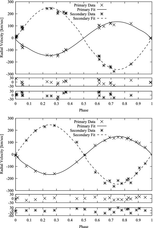
We have used the same fitting model for the rv variation, including regular proximity effects, as in Paper I. Results of the application of this program to the observed rvs are shown in Fig. 7.
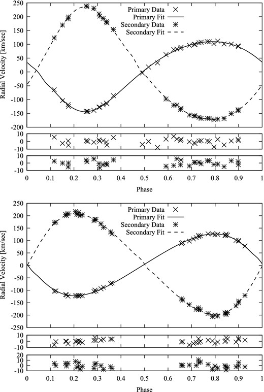
The upper panel shows our best-fitting binary rv curves for GG Lup, with residuals plotted below. The residuals of the stronger primary lines are less than those of the secondary. The former appear consistent with the random scatter in individual line measures of less than ∼6 km s−1 amplitude. In the lower panel we have plotted a similar fitting to the data of Andersen et al. (1993). The change in shape of the curves, due to the apsidal advance, can be noticed. The scatter in residuals appears comparable, in general, although that for the primary may be somewhat less in the results of Andersen et al. (1993).
2.4 Line profiles
In view of the suspected oscillatory behaviour discussed above, we sought to check for evidence of this in the line profiles (see e.g. De Cat 2002, for a review). Using the numerical model's rv parameters given in the previous subsection, the spectral response covering an 8 Å range around the He i 6678 feature was shifted to the primary star's reference frame. Results are shown in Fig. 8. An additional distorting effect on the primary profile corresponding to an eclipse phase may be seen at the top of this figure. However, any irregularity in the primary line's behaviour through the rest of the phase range may be regarded as intrinsic.
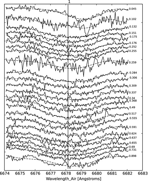
The series of He i profiles are labelled on the right with their orbital phase. The vertical spacing has been adjusted to allow feature visibility. The vertical tick marks are spaced at intervals of 10 per cent of the mean continuum. In this way it can be seen that central line depths reach to typically ∼5 per cent of the continuum.
Frequency decomposition was calculated for the wavelength window shown in Fig. 8. The amplitudes and phases of a few of the best-fitting lower frequency contributions were considered in relation to their possible dependence on orbital phase. An anomaly near orbital phase 0.1 was noticed, and this might relate to the ‘heartbeat’ effect noted in Fig. 6. But otherwise, the amplitudes showed no clearly discernible pattern, against their sizeable inherent scatter, that could be associated with a multiple of the orbital frequency. The phases of these low frequency contributions similarly suggested that the line generally tends to remain predominantly symmetrical about its centre. We thus found little clear evidence of any systematic frequency-dependent behaviour in these line profiles. Andersen et al. (1993) indicated that some of the lines they examined were not consistent with the expected trend, without expanding on possible causes.
As a check on our decomposition, the reverse transformation has been given in Fig. 8 as dashed lines for each measured orbital phase. Any regular variations of oscillation with the orbital phase should become visible in that way. But the data-quality, in the present set of spectrograms, appears of insufficiently high S/N quality to enable a detailed analysis of line profile variations with reliability. Nevertheless, superficial indications of non-constancy to the profiles of the primary (in particular), merit follow-up research.
2.5 Rotational velocities
For comparison purposes, a useful direct estimate of the synchronous rotation velocity for uniformly rotating spherical stars in circular orbits can be shown to be given by vsync = 50.6R/P, where R is the stellar radius in solar units and P is the orbital period in days. This would yield 66.2 and 49.0 km s−1 for primary and secondary values of vsync.
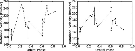
Measured rotation speeds are shown in Fig. 9. The mean apparent rotation speed of the primary at 102.6 ± 9.5 km s−1 is not far from a 3/2 resonance with the value corresponding to synchronism with the mean orbital speed, but it is still some 15 per cent greater than locking at the periastron. This has to be seen against the complications already mentioned, associated with (non-radial) pulsational effects. These imply not only that the measured line widths may arise from effects additional to the simple rotation of a near-spherical body, but that the additional role of a κ-mechanism may sustain motions that would otherwise become damped out. The scatter of results in Fig. 9 impede a clear view of any such possible phase-dependent effects, though the rotation of the primary appears generally greater in the first half of the orbital cycle than the second.
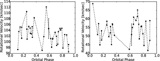
Primary and secondary rotational velocities for GG Lup. Due to the Rossiter–McLaughlin effect the interpretation of values close to phases 0.0 and 0.5 will be uncertain.
For the secondary, however, the mean rotation speed of 55.3 ± 7.2 km s−1 appears in a more expectable range, i.e. enhanced from the mean synchronization, due to greater tidal interaction near periastron, but not at the highest possible value in that respect.
2.6 Absolute parameters
Absolute parameters for GG Lup, derived from combining the foregoing photometric and spectroscopic results and Kepler's third law, are listed in Table 7. The mean photometric parallax (equation 3.42 in Budding & Demircan 2007) of 155 pc is within a reasonable error estimate of 20 pc to the astrometric value 167 pc given by HIPPARCOS.
Adopted absolute parameters for the GG Lup system. Formal errors are shown by parenthesized numbers to the right and relate to the least significant digits in the corresponding parameter values.
| Parameter | Value |
|---|---|
| Period (d) | 1.849 5927 |
| Epoch (HJD) | 2448349.0625 |
| Mags V, (B − V), (V − J) | 5.589; −0.099; −0.530 |
| Vel. amplitudes K1,2 (km s−1) | 127.5(1.0); 201.0(1.6) |
| Star separation A (R⊙) | 12.01(0.09) |
| System vel. Vγ (km s−1) | 4.0(1.0) |
| Masses M1,2 (M⊙) | 4.16(0.12); 2.64(0.12) |
| Radii R1,2 (R⊙) | 2.42(0.05); 1.79(0.04) |
| Surface grav. g (log cgs) | 4.28(0.04); 4.30(0.05) |
| Prim. mag. V1 | 5.84(0.03) |
| Sec. mag. V2 | 7.29(0.03) |
| Prim. temp. Te,1 (K) | 13 000(300) |
| Sec. temp. Te,2 (K) | 10 600(300) |
| Distance (pc) | 160(20) |
The absolute parameters of Table 7 are close to those of Andersen et al. (1993),1 particularly for the primary component, where the mass and radius values come well within our own error limits, and almost within those given by Andersen et al. Even for the secondary, whose properties are less well-determined, the differences in mass and radius are almost within our error measures. Given that the masses depend on the cube of size determinations, however, the very low error estimates of Andersen et al. appear questionable. Andersen et al. (1993) laid weight on these parameters in making inferences about the composition of young early-type stars like those of GG Lupi, which, in turn, have interesting implications for the origin of Gould's Belt stars. This point is taken up in Section 4, below.
3 μ1 Sco
The bright and hot young close binary μ1 Sco (= HD 151890, HIP 82514; V ≈ 2.98, B − V ≈ −0.16, U − B ≈ −0.85, V − J ≈ −0.48, V − H ≈ −0.50, V − K ≈ −0.72) was found to be a spectroscopic binary already over a century ago by S. I. Bailey (cf. Pickering 1896). Its membership of the Sco–Cen OB2 Association (Blaauw 1964; Preibisch & Mamajek 2008) has been adopted by many previous authors, who have used a corresponding age estimate to constrain modelling. The sky location RA (2000) = |$\mathrm{16^h 51^m 52{^{\rm s}_{.}}23}$|, Dec. (2000) = −38°02′50.″6, distance ∼160 ± 20 pc and proper motions (μαcos δ ≈ −11, μδ ≈ −22 mas yr−1) imply that the star is now located several degrees east of the main UCL concentration of the association on the sky, just ∼4° from the central plane of the Disc.
As with GG Lup, it was quite a long time after the original binary identification when Rudnick & Elvey (1938) demonstrated eclipses, using an early-type of photoelectric photometer. This was quickly followed by the van Gent (1939) photographic light curve. The history of observations of the binary was recently reviewed by van Antwerpen & Moon (2010; hereafter vAM), whose fig. 1 gives an interesting montage of seven light curves published between 1938 and 2009. The typical scatter in this montage is a few hundredths of a magnitude. These might be understood in terms of the available accuracies of older generation light detectors, particularly photographic ones. The phase range after the secondary minimum to around the second quadrature shows a larger than normal scatter, however, suggestive of some inherent additional light fluctuations.
The scatter about the fitting to the HIPPARCOS light curve (ESA 1997) is generally less than that which appears in vAM's fig. 1, but it is still appreciably larger than typical (∼0.01 mag, see our Fig. 10, for example), and it may have some systematic trends, more noticeably in the first half of the phase cycle in this data set.
3.1 Photometry and analysis
The uniformly obtained HIPPARCOS data (ESA 1997), was published with the ephemeris Min I = 2448 500.1010 + 1.446 26E. This may be compared with that of vAM who gave Min I = 2449 534.1770 + 1.446 2700E, after combining several light curves spanning a 70 yr interval. There appeared no definite evidence for any systematic variation of period beyond the sixth digit after the decimal point (in units of d) clearly distinguished in previous literature, so we adopted the light elements of vAM for our analysis. In Fig. 11 we show recent relatively high accuracy times of minima obtained within the southern binaries programme of the RASNZ VSS that support this point, although with some suggestion of a slight tendency to period increase.
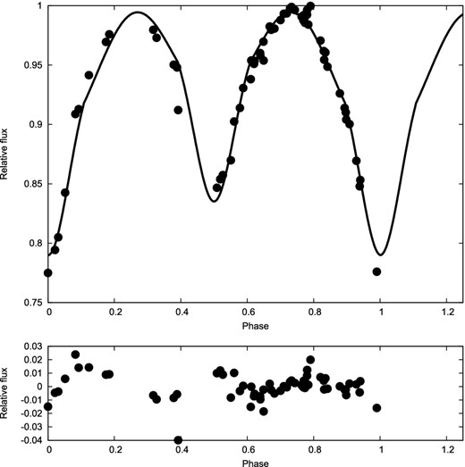
The optimized model shown in Fig. 12, together with the averaged and normalized light curve of vAM, corresponds to the parameters listed to the right in Table 8. The temperatures in this table are influenced by the values considered by vAM, as also the adopted mass-ratio. vAM argued that the photometric data would allow appreciable variation in the assigned temperatures. On the other hand, the Sahade & Garcia (1987) fitting of the UV continua appeared to give a relatively firm determination of the primary temperature (25 000 K).
Curve-fitting results for V photometry of μ1 Sco. Error estimates are given as bracketed numbers referring to the last significant digit.
| Parameter | Value | |
|---|---|---|
| HIP | vAM | |
| Th (K) | 24 000 | 24 000 |
| Tc (K) | 17 000 | 17 000 |
| M2/M1 | 0.627 | 0.627 |
| L1 | 0.48(7) | 0.55(6) |
| L2 | 0.52(7) | 0.45(6) |
| r1 | 0.350(6) | 0.311(2) |
| r2 | 0.373(8) | 0.366(3) |
| i (deg) | 62.6(8) | 64.4(3) |
| e | 0.0 | 0.0 |
| u1 | 0.24 | 0.24 |
| u2 | 0.30 | 0.30 |
| Δϕ0(deg) | 0.0 | 0.0 |
| χ2/ν | 1.03 | 0.94 |
| Δl | 0.01 | 0.007 |
Although the mean (s.d.) dispersion of 0.01 mag appears about typical for a HIPPARCOS data set, here with only 62 points, the scatter seems not so uniformly distributed, echoing suggestions from earlier observers of an intrinsic variability beyond that associated with a regular eclipsing binary system. The two fittings of Table 8 are appreciably different, in comparison with the formal error estimates, suggesting some lack of modelling adequacy to cover the inherent complexity of the system.
In agreement with previous authors is our initial result that the secondary star is larger than the primary, and certainly larger than a normal main-sequence relationship would imply for the given primary radius and the secondary's much lower mass, that we confirm later. The system must therefore be in a state involving binary (i.e. interactive) evolution. The relatively large masses, high primary surface temperature, and proximity of the components make this a very atypical arrangement for a ‘classical’ Algol binary, however. The similarity of the period and mass-ratio to that of GG Lup may be noticed, though it quickly becomes clear that μ1 Sco must be in quite a different condition. The marked proximity effects of the light curve in Fig. 12 cannot be explained by two near-main-sequence stars.
The scatter of individual light curves, like that shown in Fig. 10 , and the historic ones reviewed by vAM can be considerably reduced by averaging (‘normalizing’) data over short phase ranges. In this way, the data set shown in Fig. 12 was produced by vAM, and analysed to find parameters that are similar to those we have found and listed in Table 8. Our secondary relative radius appears larger than that of vAM, but otherwise the parameters (ours and vAM’s) are generally comparable.
HIPPARCOS V photometry of μ1 Sco and model fitting with residuals below (see Section 4.1 for details).
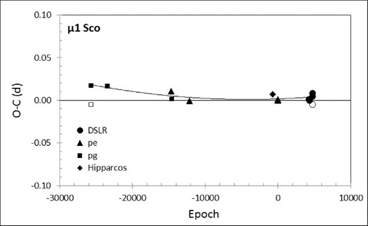
Times of minima for μ1 Sco (primary, filled symbols; secondary, open). We have added our own recent DSLR timings to the historic ones reported by vAM. There is a suggestion of a slight period increase indicated by the parabolic fit, but the second-order term in the epoch number is less than 10−10 and clearly low when placed alongside comparable Algol systems (Kreiner & Ziółkowski 1978).
Normalized V-band photometry of μ1 Sco, after van Antwerpen & Moon (2010), and model fitting.
BVR photometry of selected eclipsing binaries of the southern sky by members of the VSS section of the RASNZ (cf. Section 2.1) has included μ1 Sco, using the same (DSLR) equipment. The light curves are shown in Fig. 13, where we also show optimal fits to the reduced B, V and R data sets and the V residuals. The parameters going with these fits are listed in Table 9, where similarity of the fitting to the collected literature data of vAM (Table 8, right) may be noticed. The fractional luminosities of the two components (L) in the optical region can be seen to be comparable. This also follows from the temperature and radius ratios, given that the BVR filters fall into the ‘Rayleigh–Jeans’ radiation regime (approximately). The slight preference in the results for L1 > L2 is suggestive that the assigned value of Tc may be slightly too high.
Radau model fitting (Rhodes & Budding 2014) to DSLR BVR light curves of μ1 Sco. The residuals from the V fitting are shown below.
Curve-fitting results for this paper's BVR photometry of μ1 Sco.
| Parameter | Value | ||
|---|---|---|---|
| B | V | R | |
| Th (K) | 24 000 | ||
| Tc (K) | 17 000 | ||
| M2/M1 | 0.55 | ||
| L1 | 0.52(3) | 0.52(3) | 0.52(4) |
| L2 | 0.48(3) | 0.48(3) | 0.48(4) |
| r1 | 0.311(2) | ||
| r2 | 0.369(3) | ||
| i (deg) | 64.3(3) | ||
| u1 | 0.29 | 0.25 | 0.21 |
| u2 | 0.35 | 0.30 | 0.25 |
| Δϕ0(deg) | 0.0 | 0.0 | 0.0 |
| χ2/ν | 1.03 | 1.01 | 1.02 |
| Δl | 0.006 | 0.0055 | 0.007 |
3.2 Spectroscopy
Our spectroscopic data were gathered using the HERCULES spectrograph with arrangements essentially similar to those described in Section 2.2. The data were gathered over three allocations at MJUO in 2006 May, 2010 August and 2011 August. A new SI600s-type camera replaced the SITe one used for the 2006 data. The high brightness of μ1 Sco entailed that exposures could be taken in relatively poor weather. Seeing conditions would therefore often be relatively poor and the S/N for several of the 24 spectrograms is not as high as the brightness of the star might suggest. In fact, when recording spectral images with HERCULES it is normal to allow the integrated photon count, which is displayed as the exposure time (t) proceeds, to be terminated at a value corresponding to a continuum S/N of ∼100 for the lower used orders: typically ∼50–200 s (cf. Section 2.2).
A compromise is involved here in that while the S/N varies in proportion only to |$\sqrt{t}$|, longer exposures for binaries of shorter period will smear out the Doppler shifting and lose velocity resolution. The rotational broadenings for μ1 Sco are about double (primary) or treble (secondary) those of GG Lup, however (Section 3.4). The precision with which line positions can be specified is correspondingly reduced, as is reflected in the dispersion panels of Fig. 14. The data were reduced using the (revised) software hrsp 5 (Skuljan, private communication), further analysis being then carried out using iraf.
3.3 Radial velocities
The central issue of locating lines for rapidly rotating early-type stars was discussed in Sections 2.2 and 2.3 above. Additional complications associated with the ongoing interactive evolution of the system are likely to be also present in the case of μ1 Sco. Profile fitting using ‘dish shaped’ functions convolved with Gaussians set against slightly sloping continua was attempted, but the large broadening of the generally not intrinsically strong and possibly distorted features resulted in relatively poor determination of positions. The lines listed in Table 10 provide a guide to what was dealt with, but in many cases only the He i lines allow shifts to be determined with an acceptable accuracy of several km s−1.
Spectral lines of μ1 Sco which were used for rv determination.
| Species | Order no. | Wavelength | Comment |
|---|---|---|---|
| He i | 85 | 6678.149 | strong p, moderate s |
| He i | 97 | 5875.65 | strong p, usable s |
| He i | 113 | 5015.67 | weak p, very weak s |
| He i | 115 | 4921.93 | moderate p, weak s |
| He i | 121 | 4713.201 | weak p, weak s |
| Species | Order no. | Wavelength | Comment |
|---|---|---|---|
| He i | 85 | 6678.149 | strong p, moderate s |
| He i | 97 | 5875.65 | strong p, usable s |
| He i | 113 | 5015.67 | weak p, very weak s |
| He i | 115 | 4921.93 | moderate p, weak s |
| He i | 121 | 4713.201 | weak p, weak s |
The final set of rv measurements, which were derived from the fitting function's centroid positions, is given in Table 11. Dates and velocities and have been corrected to heliocentric values as before and are shown in Fig. 14. Although the rvs are again listed with one significant decimal place in Table 11, this gives an overoptimistic impression of the accuracy of the determination (cf. Section 2.3).
The upper panel shows the best-fitting binary rv curves for our observations of μ1 Sco, with the residuals plotted below. The excursions of the stronger primary lines are slightly less than those of the secondary. The former appear consistent with the random scatter in the individual measures of less ∼12 km s−1 amplitude. The lower panel shows our fitting to the rv data assembled by vAM (2010). Again we notice a comparable scatter in the residuals, relating to the difficulties of locating the few, very broad and shallow lines.
Radial velocity data for μ1 Sco.
| No | Phase | RV1 | RV2 |
|---|---|---|---|
| (km s−1) | (km s−1) | ||
| 1 | 0.0041 | 8.5 | 1.7 |
| 2 | 0.0070 | – | 16.2 |
| 3 | 0.0097 | – | 14.4 |
| 4 | 0.0445 | − 56.9 | 90.3 |
| 5 | 0.0496 | − 81.8 | 72.3 |
| 6 | 0.0501 | − 64.1 | 92.0 |
| 7 | 0.0525 | − 79.7 | 76.6 |
| 8 | 0.2313 | − 143.4 | 243.1 |
| 9 | 0.2615 | − 147.8 | 244.2 |
| 10 | 0.3087 | − 150.4 | 203.1 |
| 11 | 0.3116 | − 140.8 | 218.5 |
| 12 | 0.3524 | − 113.4 | 214.4 |
| 13 | 0.3682 | − 96.4 | 205.1 |
| 14 | 0.3701 | − 101.6 | 203.8 |
| 15 | 0.6114 | 102.8 | − 152.6 |
| 16 | 0.6141 | 104.6 | − 150.6 |
| 17 | 0.6143 | 80.9 | − 179.3 |
| 18 | 0.6466 | 95.2 | − 229.1 |
| 19 | 0.6953 | 118.3 | − 237.5 |
| 20 | 0.6981 | 123.4 | − 245.6 |
| 21 | 0.7217 | 108.5 | − 278.3 |
| 22 | 0.8470 | 119.8 | − 217.0 |
| 23 | 0.9887 | − 1.1 | – |
| 24 | 0.9914 | − 3.2 | – |
3.4 Rotation velocities
Measured rotational speeds are shown in Fig. 15. The mean apparent rotation speed of the primary at 191.5 km s−1 is faster than synchronization by a factor of approximately 1.5. For the secondary however, the mean rotation speed of 165.0 km s−1 appears closer to synchronization, though still ∼10 per cent higher.
Primary and secondary rotational velocities for μ1 Sco. Due to the Rossiter–McLaughlin effect the interpretation of values close to phases 0.0 and 0.5 will be uncertain.
The high rotation speed of the primary is again an issue, since the synchronization time-scale is expected to be fairly short in comparison to the main-sequence time for close pairs, as noted in Section 2.1. The circumstance of ongoing interactive evolution will significantly complicate the angular momentum history, however, so that it is not obvious that standard models can be applied to μ1 Sco.
3.5 Absolute parameters
Our derived absolute parameters for μ1 Sco are listed in Table 12.
Adopted absolute parameters for the μ1 Sco system. Formal errors are shown by parenthesized numbers to the right and relate to the least significant digits in the corresponding parameter values.
| Parameter | Value |
|---|---|
| Period (d) | 1.446 27 |
| Epoch (HJD) | 2449534.177 |
| Mags. V, (B − V), (U − B) | 2.98; −0.016; −0.85 |
| Vel. amplitudes K1,2 (km s−1) | 140(5); 257(10) |
| Star separation A (R⊙) | 12.6(0.5) |
| System vel. Vγ (km s−1) | −6(3) |
| Masses M1,2 (M⊙) | 8.3(1.0); 4.6(1.0) |
| Radii R1,2 (R⊙) | 3.9(0.2); 4.6(0.3) |
| Surface grav. g (log cgs) | 4.17(0.10); 3.77(0.12) |
| Prim. mag. V1 | 3.63(0.04) |
| Sec. mag. V2 | 3.85(0.05) |
| Prim. temp. Te,1 (K) | 24 000(1000) |
| Sec. temp. Te,2 (K) | 17 000(700) |
| Distance (pc) | 130(20) |
The distance derived from the photometric parallax (equation 3.42 in Budding & Demircan 2007), using the data of Table 12, is somewhat smaller than the HIPPARCOS value of 156 pc (van Leeuwen 2007), which lies just outside the upper 1σ range of the photometric distance estimate. The photometric estimate has neglected interstellar reddening, however, and, although small at this distance, AV can be taken to be ∼0.07 mag (vAM), which would allow the two distance estimates to agree within the errors of the determination. Either distance would be consistent with the range given for the Scorpius region of the Sco–Cen OB2 Association (De Zeeuw, Hoogerwerf & de Bruijne 1999; Preibisch & Mamajek 2008).
The absolute parameters given in Table 12 are generally within their error estimates of those of vAM, although outside the errors given by vAM. It can be seen from Figs 12–14 that the scatter in the photometric and spectroscopic sets, both vAM's and ours, is ∼10 per cent that of their amplitudes. The precision of parameters given by vAM therefore seem to be overoptimistic, as our closer checks confirm – particularly for the masses.
4 DISCUSSION
The parameters for the stars of GG Lup given in Table 7 suggest a relatively young pair, and this is supported by the physical characteristics of the system in which a high rotational velocity of the primary has still not been eroded by its frequent close encounters with its companion in the unusually eccentric orbit. In Fig. 16 we plot stellar radii versus time using the data of the Padova group (Bressan et al. 2012) with a solar composition. The derived radii and masses of the components turn out to be consistent with each other and with an age of approximately 33 Myr. This is not so young as the age estimated by Andersen et al. (1993), and indeed significantly greater than representative values for the UCL region (∼15 Myr; Preibisch & Mamajek 2008).
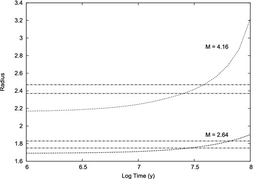
Radial evolution of the stars in GG Lup. The 1σ error bounds of the measured radii are shown as horizontal lines.
Andersen et al. (1993) argued for a metal-composition for the stars of GG Lup significantly below solar, putting particular weight on their derived relatively high gravity for the secondary star. Our findings do not give unequivocal support to that argument, even though we have re-analysed the photometric and spectroscopic data used by Andersen et al. as well as our own data and find a good measure of agreement in the basic parameters of the fitting functions used to match all the data sets, together with comparable levels of scatter in the residuals. Whilst the arguments of Andersen et al. are of interest, particularly in relation to the problem of the origin of Gould's Belt (cf. e.g. Grenier 2004), we believe that a more realistic assessment of the parameter errors, especially of the masses, do not allow GG Lup, at least not in isolation, to be used as a reliable discriminant between alternative composition possibilities. Solar composition models can provide a self-consistent picture for the observed properties. In fact, if we were to apply the lower metal abundance value considered by Andersen et al. (Z = 0.01) the starting radii in Fig. 16 are lowered and the time taken to achieve the presently observed values is increased by about 3 Myr, increasing the disparity with the average age of the UCL region stars. But the indications of pulsational instability or anomalously high rotation in the envelope of at least the primary component, given the unexpectedly persisting orbital eccentricity, may render comparisons with normal single stars inappropriate.
On the other hand, for the Sco OB2 Association member μ1 Sco, the radius of a star of the same mass as that found for the primary (8.3 M⊙) agrees closely with that measured for the star (Fig. 17). This agreement suggests that the primary has been relatively little affected by the Case A-type evolution of the secondary. The Case A scenario, considered by Giannuzzi (1983), Stickland, Sahade & Henrichs (1996) and others, involving appreciable mass-loss from the system in the relatively recent past, arises because of the anomalous mass, near Roche lobe-filling, and high-luminosity secondary star and therefore generally Algol-like condition of the system, yet with the absence of significant period variation.
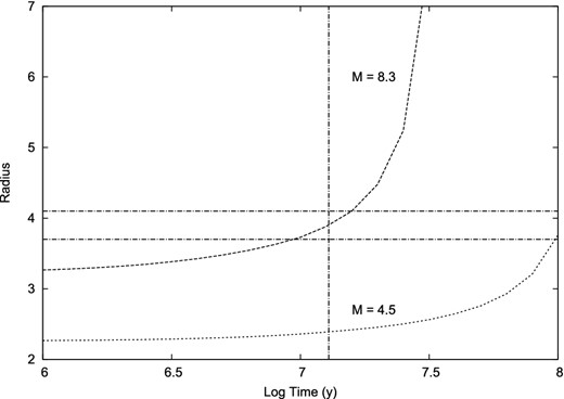
Radial evolution of a main-sequence star with the present mass of the primary of μ1 Sco. The 1σ limits within which its measured radius should lie are shown as horizontal lines. For comparison, we show also the radial evolution of a star of mass 4.5 M⊙.
In that scenario, the secondary must have lost at least ∼4 M⊙ of its original mass. The primary's condition, meanwhile, remains measurably close to what it would have been as a single star at its present mass. If all the lost matter had been transferred, the primary would have started by following the lower track in Fig. 17. But it is difficult to see how it could have then reached its present radius of about 4 R⊙ whilst maintaining stability on a Kelvin time-scale in accordance with the insignificant period variation. A plausible implication is that the very high surface temperature of the primary causes sufficient ionizing absorption in matter shed from the secondary that radiation pressure expels such plasma from the system via the external Kepler ring (De Loore & Van Rensbergen 2005).
Generous allocations of time on the 1m McLennnan Telescope and HERCULES spectrograph at the MJUO in support of the Southern Binaries Programme have been made available through its TAC and supported by its Director, Dr K. Pollard and previous Director, Professor J. B. Hearnshaw. Useful help at the telescope were provided by the MJUO management (A. Gilmore and P. Kilmartin). Considerable assistance with the use and development of the hrsp software (leading up to the latest version 5) was given by its author Dr J. Skuljan.
Encouragement and support for this programme has been shown by the School of Chemical and Physical Sciences of the Victoria University of Wellington, as well as the RASNZ and its VSS section (http://www.variablestarssouth.org). We thank VSS Director Tom Richards for advocating DSLR photometry in support of the Southern Binaries Programme.
An unnamed reviewer made helpful comments causing us to check our results as well as compare them with others more carefully, resulting in an improved presentation.
Visiting Astronomer, Department of Physics, and Astronomy, University of Canterbury, Private Bag 4800, Christchurch 8140, New Zealand.
Andersen et al. (1993) gave component masses of 4.12 ± 0.04 and 2.51 ± 0.02 M⊙, and radii of 2.38 ± 0.03 and 1.72 ± 0.02 R⊙.
