


Abstract
We present a detailed analysis of a H2-bearing metal-rich sub-damped Lyman α system at zabs = 0.10115 towards the radio-loud quasar J0441−4313, at a projected separation of ∼7.6 kpc from a star-forming galaxy. The H2, |${\rm C\,{\small \rm I}}$| and |${\rm Na\,{\small \rm I}}$| absorption are much stronger in the redder of the two components seen in the Hubble Space Telescope/Cosmic Origins Spectrograph spectrum. The best single-component fit to the strong H2 component gives log N(H2) = 16.61 ± 0.05. However, possible hidden saturation in the medium-resolution spectrum can allow for log N(H2) to be as high as 18.9. The rotational excitation temperature of H2 in this component is 133|$^{+33}_{-22}$| K. Photoionization models suggest 30–80 per cent of the total N(H i) is associated with the strong H2 component that has a density ≤100 cm−3 and is subject to a radiation field that is ≤0.5 times the Galactic mean field. The Very Long Baseline Array 1.4 GHz continuum image of the radio source contains only 27 per cent of the arcsecond scale emission. Using a previously published spectrum, no 21-cm absorption is found to be associated with the strong H2 component. This suggests that either the N(H i)) associated with this component is ≤50 per cent of the total N(H i)) or the gas covering factor is ≤0.27. This is consistent with the results of the photoionization model that uses ultraviolet radiation due to stars in the associated galaxy. The 21-cm absorption previously reported from the weaker H2 component suggests a spin temperature of ≤90 K, at odds with the weakness of H2, |${\rm C\,{\small \rm I}}$| and |${\rm Na\,{\small \rm I}}$| absorption in this component. From the inferred physical and chemical conditions, we suggest that the gas may be tracing a recent metal-rich outflow from the host galaxy.
1 INTRODUCTION
Damped Lyman α systems (DLAs) and sub-DLAs are by definition absorbers with neutral hydrogen column density N(H i))≥ 2 × 10²⁰ and ≥1 × 1019 cm−2, respectively (see Wolfe, Gawiser & Prochaska 2005, for a review). These high H i column density absorbers trace the bulk of the H i at 2 < z < 3 (Péroux et al. 2005; Noterdaeme et al. 2009b, 2012), and can in principle contribute significantly to the global star formation rate (Wolfe, Prochaska & Gawiser 2003; Srianand et al. 2005). While they have been conjectured to be originating from gas associated with high-z galaxies/protogalaxies, their direct connection with galaxies is not yet well understood. The link between DLAs/sub-DLAs and galaxies can be established by directly detecting the host galaxies and/or showing that the prevailing physical conditions in the absorbing gas are consistent with those seen in a typical galactic interstellar medium (ISM).
Because of difficulties associated with detecting high-z galaxies that are close to bright quasi-stellar object (QSO) sightlines, our understanding of the physical conditions in DLAs/sub-DLAs at z > 1.8 is primarily based on optical absorption line studies of low-ionization metal transitions and, in a few cases, H2, HD and CO molecular transitions (e.g. Varshalovich et al. 2001; Ledoux, Petitjean & Srianand 2003; Noterdaeme et al. 2008a,b, 2009a; Srianand et al. 2008). The observed high-J excitations of H2 at high-z are consistent with a strong ultraviolet (UV) field suggesting in situ star formation, while the typical temperatures and densities of the H2 components are 153 ± 78 K and 10–200 cm−3, respectively (Srianand et al. 2005). The gas producing H2 absorption probably traces diffuse molecular gas in the form of compact clouds (Balashev et al. 2011) and contains only a small fraction of the H i measured using the DLA profile (Srianand et al. 2012).
The H i 21-cm absorption line provides a complementary way to probe the physical conditions in the H i gas. If detected it can be used to investigate (1) the thermal state of H i gas, as 21-cm optical depth is a good tracer of the gas kinetic temperature being inversely proportional to the spin temperature (Kulkarni & Heiles 1988); (2) the parsec-scale structure in the absorbing gas via milliarcsecond (mas) scale spectroscopy (Srianand et al. 2013); (3) the magnetic field in the cold neutral medium (CNM) using Zeeman splitting (Heiles & Troland 2004); (4) the filling factor of cold gas in the ISM. Unfortunately, 21-cm detections from DLAs at high-z are very rare (see Srianand et al. 2012; Kanekar et al. 2014, for recent compilations). This lack of 21-cm detection is attributed to the gas being warm and/or to partial coverage of the background radio sources by the absorbing clouds.
The effect of covering factor and the size of absorbing clouds can in principle be quantified by searching for 21-cm absorption in DLAs/sub-DLAs with H2 detections. In our Galactic high latitude sightlines, a correspondence between H2 and 21-cm absorption is well established when log N(H2) ≥ 15.8 (see Roy, Chengalur & Srianand 2006). Based on this study, we know that the gas kinetic temperature measured from the rotational level populations of H2, T01, traces the H i spin temperature, Ts. Therefore, in that case the lack of 21-cm absorption from a gas showing low rotational temperature of H2 cannot be naturally attributed to the gas being warm. However, high-z DLAs with H2 detection towards radio-bright QSOs (with flux density in excess of 100 mJy at the redshifted 21-cm frequencies), at appropriate zabs (enabling 21-cm absorption search) are rare. Even the five cases where this is possible, do not follow the relationship between 21-cm and H2 absorption (see Srianand et al. 2012). This lack of correspondence may mean that only a small fraction (i.e. ≤10 per cent) of the total H i is associated with the H2 components or that the H2 clouds are too small (i.e. <15 pc) to cover even the unresolved radio components at mas scales. To resolve this, mas scale very long baseline interferometry (VLBI) imaging of the background radio source is essential to determine the covering factor (see e.g. Gupta et al. 2012). A good understanding of these issues is important to interpret the results of on-going and future 21-cm absorption line surveys, as well as surveys of H2 in DLAs/sub-DLAs.
Low-z DLAs and sub-DLAs are ideal targets to address the above issues. This is because (1) for a given angular scale one will be probing a much smaller physical scale, where the covering factor issues may have minimum effects (see Curran et al. 2005); (2) in the case of 21-cm detections one will be able to carry out VLBI spectroscopic observations to get spatial scales in the absorbing H i gas (Borthakur et al. 2010; Srianand et al. 2013); (3) direct association of the absorbers with the galaxies responsible for the absorption is possible. The last one will allow us to relate the inferred spatial scales in the absorbing gas to its location with respect to the galaxy (i.e. in the star-forming regions or in the halo). Srianand et al. (2013) have demonstrated the presence of structures in the 21-cm optical depth on parsec scales in the ISM of a low-z galaxy. In such cases of the background radio source being structured, the spatial variation of the H i gas opacity can be studied using VLBI spectroscopy.
UV spectroscopic surveys with the Hubble Space Telescope (HST) are identifying significant numbers of low-z DLAs and sub-DLAs (Meiring et al. 2011; Rao et al. 2011; Battisti et al. 2012). Thanks to the Cosmic Origins Spectrograph (COS) on board the HST, there have been three recent cases of H2 detection in low-z (i.e. z < 0.6) DLAs (Crighton et al. 2013; Oliveira et al. 2014; Srianand et al. 2014). Recently by a careful search in 27 low-z (i.e. z < 1) DLAs and sub-DLAs towards 26 QSOs, using HST/COS archival spectra, Muzahid, Srianand & Charlton (2014) have reported seven new H2 detections. With the largest sample to date (10) of H2 detections at low-z, they find ≳2 times higher H2 incidence rate at low-z compared to high-z. The H2 components in their sample have typical temperatures of 133 ± 55 K. From photoionization models and the lack of high-J excitations, the authors have shown that the prevailing radiation field is much weaker than the Galactic UV radiation field, in contrast with the results at high-z. Moreover, the large impact parameters of the host-galaxies (>15 kpc) for majority of their systems strongly suggest that the H2-bearing gas is not related to star-forming discs but probably stems from extended halo gas.
Among the low-z sample of H2 absorbers of Muzahid et al. (2014), two are towards radio-loud QSOs, which in principle facilitate detailed study of the cold gas in these absorbers. However, the redshift of one of these systems falls in the frequency range affected by radio frequency interference at available radio telescopes. The other system is the subject of detailed study in this paper. This paper is organized as follows. In Section 2, we give details of the observations and data reduction process. The physical properties of the system as derived from the absorption lines are discussed in Section 3. The properties of the associated galaxy and their comparison with that of the absorber are discussed in Section 4. Section 5 explains the results from our photoionization modelling of the absorber. In Section 6, we focus on the Very Long Baseline Array (VLBA) mas scale imaging of the background radio source at 1.4 GHz and the previously reported 21-cm absorption from the cold gas using the Australia Telescope Compact Array (ATCA). Lastly, we summarize our results in Section 7. Throughout this paper we use a flat cosmology with H0 = 70 km s−1 Mpc−1 and Ωm = 0.27.
2 OBSERVATIONS AND DATA REDUCTION
The QSO J044117.3−431343 (zem = 0.59378; also known as PKS 0439−433 and henceforth J0441−4313) was observed using COS during HST cycle-19, under program ID: 12536 (PI: V. Kulkarni). These observations consist of G130M far-UV grating integrations (5.3 ks) at a medium resolution of R ∼ 18 000 [full width at half-maximum (FWHM) ∼ 18 km s−1]. The data were retrieved from the HST archive and reduced using the calcos pipeline software. The individual reduced x1d files were first flux calibrated. Then the alignment and co-addition of the separate exposures were carried out using the software developed by Danforth et al. (2010).1 The exposures were weighted by the integration time while co-adding the flux calibrated data. The final co-added spectrum covers the observed wavelength range 1131–1435 Å and has a signal-to-noise ratio (S/N) ∼ 16–20 per resolution element. Since each COS resolution element is sampled by 6 raw pixels, we binned the spectrum by 3 pixels, which further improves the S/N per pixel. All measurements and analyses were, subsequently, performed on the binned data. Measurements are, however, found to be fairly independent of the binning. Continuum normalization was done by fitting the line-free regions with a smooth lower order polynomial.
The COS wavelength calibration is known to be uncertain at the level of 10–15 km s−1 (Savage et al. 2011; Meiring et al. 2013). Regions of the spectrum that are recorded near the edges of the detector segment are likely to have an erroneous wavelength solution (see e.g. Muzahid et al. 2014). However, in the case of the present spectrum, the velocity offsets at different wavelengths as estimated from the difference in the observed and the expected line centroids of the numerous H2 absorption lines are ≲ ±5 km s−1. Moreover, the Galactic absorption lines are found to be aligned within ≲ ±5 km s−1. The line spread function (LSF) of the COS spectrograph is not a Gaussian. Ghavamian et al. (2009) provided a characterization of the non-Gaussian LSF for COS, which was subsequently updated by Kriss (2011). We adopt this updated LSF for our Voigt profile fitting analysis. Interpolated LSF at the line centre was convolved with the model Voigt profile while fitting an absorption line using the vpfit2 code.
In addition, we use the pipeline calibrated spectrum (R ∼ 45 000, FWHM ∼ 6.6 km s−1) of QSO J0441−4313 obtained using the Ultraviolet Echelle Spectrograph (UVES) on the Very Large Telescope (VLT), available in the European Southern Observatory (ESO) archive.3 The spectra corresponding to different exposures covering our regions of interest, after applying barycentric correction, were brought to their vacuum values using the formula given in Edlen (1966). For the co-addition, we interpolated the individual spectra and their errors to a common wavelength array, and then computed the weighted mean using the weights estimated from the error in each pixel. The final spectrum covers the observed wavelength range 3732–6837 Å with S/N ∼ 40–50 per resolution element.
Furthermore, we observed the background radio source with the VLBA using the 21-cm receiver band for 1 h on 2014 August 26. The total bandwidth was 256 MHz in dual polarization (eight 32 MHz baseband channel pairs). Each baseband channel was split into 128 spectral points. Two-bit sampling and a correlator integration time of 2 s were used. The observations were carried out in nodding-style phase referencing with a cycle of ∼5 min, i.e. ∼3.5 min on source and ∼1.5 min on the phase calibrator (J0440−4333). A strong fringe finder/bandpass calibrator (DA193) was also observed at the beginning for 4–5 min. The target source was observed for ∼35 min, split into scans at different hour angles to improve the UV coverage. Data were calibrated and imaged using Astronomical Image Processing System (aips; Greisen 2003) in a standard way (see e.g. Momjian, Romney & Troland 2002; Srianand et al. 2012).
3 ABSORPTION LINE PROPERTIES OF THE SUB-DLA
The sub-DLA at zabs = 0.10115 towards J0441−4313 with log N(H i))= 19.63 ± 0.08 and log N(H2) = 16.61 ± 0.05 (Muzahid et al. 2014) presents a very interesting case for understanding the cold gas that is present around galaxies. This system was originally selected as a DLA candidate based on strong |${\rm Mg\,{\small \rm II}}$| and |${\rm Fe\,{\small \rm II}}$| absorption in the Faint Object Spectrograph (FOS) spectrum (Petitjean et al. 1996). We note that Chen, Kennicutt & Rauch (2005) derived log N(H i))= 19.85 ± 0.10 for this sub-DLA using the Space Telescope Imaging Spectrograph (STIS) G140L spectrum, consistent within 2σ of our measurement. In this section, we discuss the properties of the sub-DLA as probed by the absorption lines (metals and H2) detected in the COS and UVES spectra.
3.1 Analysis of metal lines
We detect the metal transitions |${\rm C\,{\small \rm I}}$|, |${\rm C\,{\small \rm II}}$|, |${\rm N\,{\small \rm I}}$|, |${\rm N\,{\small \rm II}}$|, |${\rm O\,{\small \rm I}}$|, |${\rm Si\,{\small \rm II}}$|, |${\rm Si\,{\small \rm iii}}$|, |${\rm P\,{\small \rm II}}$|, |${\rm S\,{\small \rm II}}$|, |${\rm Ar\,{\small \rm I}}$|, |${\rm Fe\,{\small \rm II}}$| and |${\rm Fe\,{\small \rm iii}}$| in the COS spectrum spread over a velocity range of ∼150 km s−1. Some of these absorption profiles are shown in the left-hand panel of Fig. 1. The |${\rm C\,{\small \rm II}}$|, |${\rm N\,{\small \rm II}}$|, |${\rm O\,{\small \rm I}}$|, |${\rm Si\,{\small \rm II}}$|, |${\rm Si\,{\small \rm iii}}$| and |${\rm Fe\,{\small \rm iii}}$| lines are saturated/heavily blended and hence not used in our analysis. We do not cover the |${\rm C\,{\small \rm II}}$|* λλ1335.7, 1335.6 transitions, and the |${\rm C\,{\small \rm II}}$|* λ1037 transition is heavily blended. |${\rm C\,{\small \rm I}}$|* absorption is absent and we place a 3σ upper limit on its column density using the strongest transition that is free from any blend, i.e. λ1279.9. Further, |${\rm Mg\,{\small \rm II}}$| λλ1239, 1240 and |${\rm Mn\,{\small \rm II}}$| λ1197 absorption are not detected and we use these to place 3σ upper limits on N(|${\rm Mg\,{\small \rm II}}$|) and N(|${\rm Mn\,{\small \rm II}}$|), respectively. From the Voigt profile fits to the unblended and most likely unsaturated metal lines detected in the COS spectrum, we infer two main absorbing clumps of gas at zabs = 0.10094 and 0.10119 (henceforth Component 1 and 2, respectively), ∼68 km s−1 apart (see left-hand panel of Fig. 1). We assume that all the neutral and singly ionized atoms are physically associated with the same gas cloud. Hence while fitting, the redshift and b parameter for each absorption component are tied to be the same for each of the ions, i.e. only turbulent broadening is considered. Additionally, we rejected fits with more than two components since, although having similar |$\chi ^2_{\nu }$|, they have larger values of AICC [Akaike information criteria (Akaike 1974) corrected for the finite sample size (AICC; Sugiura 1978) as given in equation (4) of King et al. (2011)] and higher errors in the parameters.
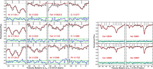
A selection of metal lines associated with the sub-DLA at zabs = 0.10115 towards J0441−4313 detected in the COS (left) and UVES (right) spectrum. Best-fitting Voigt profiles are overplotted in red. The tick marks show the component positions. The errors in flux and residuals from the fit are shown at the bottom as green lines and blue histograms, respectively.
The medium resolution of the COS spectrum is not sufficient to resolve all the different components in the absorbing gas, in particular the narrow ones. In the present case, since |${\rm Ca\,{\small \rm II}}$| and |${\rm Na\,{\small \rm I}}$| absorption lines have been detected in the high-resolution UVES spectrum (Richter et al. 2011), we can get a realistic idea of the component structure. We find that 10 and 8 components give the best fit to the |${\rm Ca\,{\small \rm II}}$| and |${\rm Na\,{\small \rm I}}$| lines, respectively (see Table 1 and right-hand panel of Fig. 1). The column densities that we obtained are consistent within errors with those reported by Richter et al. (2011). Table 2 lists the column density measurements or 3σ upper limits in the case of non-detections of the various ions. In the case of |${\rm Ca\,{\small \rm II}}$| and |${\rm Na\,{\small \rm I}}$|, to facilitate comparison between Components 1 and 2 seen in the COS spectrum, we sum the column densities in components (a)–(d) and (e)–(j), respectively.
Component-wise column densities (with errors shown in parentheses) of |${\rm Ca\,{\small \rm II}}$| and |${\rm Na\,{\small \rm I}}$| detected from the sub-DLA at zabs = 0.10115 towards J0441−4313.
| b | log N(|${\rm Ca\,{\small \rm II}}$|) | log N(|${\rm Na\,{\small \rm I}}$|) | ||
|---|---|---|---|---|
| Comp. | zabs | (km s−1) | (cm−2) | (cm−2) |
| a | 0.10084 (0.000001) | 1.55 (0.46) | 11.61 (0.04) | 11.26 (0.03) |
| b | 0.10090 (0.000003) | 4.91 (1.03) | 11.63 (0.09) | 11.16 (0.06) |
| c | 0.10093 (0.000003) | 4.44 (1.08) | 11.74 (0.08) | 10.59 (0.25) |
| d | 0.10100 (0.000005) | 8.80 (2.34) | 11.53 (0.08) | 10.46 (0.23) |
| e | 0.10108 (0.000002) | 5.88 (0.93) | 11.48 (0.06) | 11.19 (0.04) |
| f | 0.10112 (0.000002) | 1.55 (0.87) | 11.54 (0.06) | – |
| g | 0.10114 (0.000001) | 2.19 (0.20) | 12.08 (0.03) | 12.04 (0.02) |
| h | 0.10118 (0.000002) | 4.37 (1.16) | 11.72 (0.05) | 11.33 (0.06) |
| i | 0.10122 (0.000005) | 0.84 (0.80) | 11.37 (0.16) | 10.67 (0.16) |
| j | 0.10125 (0.000007) | 5.35 (2.56) | 11.34 (0.13) | – |
Component-wise column densities (with errors shown in parentheses) of metals detected from the sub-DLA at zabs = 0.10115 towards J0441−4313.
| log N (cm−2) | ||||
|---|---|---|---|---|
| Ion (X n) | Component 1a | Component 2b | Total | [X n/H]c |
| H i | – | – | 19.63 (0.08) | – |
| |${\rm C\,{\small \rm I}}$| | 13.31 (0.14) | 14.01 (0.04) | 14.09 (0.04) | – |
| |${\rm C\,{\small \rm I}}$|* | ≤13.40 | ≤13.50 | ≤13.75 | – |
| |${\rm N\,{\small \rm I}}$| | 14.64 (0.02) | 14.71 (0.02) | 14.98 (0.02) | −0.48 (0.08) |
| |${Na\,{\small i}}^{d}$| | 11.60 (0.04) | 12.18 (0.02) | 12.28 (0.02) | – |
| |${\rm Mg\,{\small \rm II}}$| | ≤15.30 | ≤15.30 | ≤15.60 | ≤0.37 |
| |${\rm P\,{\small \rm II}}$| | 13.00 (0.11) | 13.29 (0.07) | 13.47 (0.06) | +0.43 (0.10) |
| |${\rm S\,{\small \rm II}}$| | 14.65 (0.04) | 14.79 (0.03) | 15.03 (0.02) | +0.28 (0.08) |
| |${\rm Ar\,{\small \rm I}}$| | ≤12.27 | 13.22 (0.12) | 13.27 (0.14) | −0.76 (0.16) |
| |${Ca\,{\small ii}}^{d}$| | 12.24 (0.04) | 12.45 (0.03) | 12.66 (0.02) | – |
| |${\rm Mn\,{\small \rm II}}$| | ≤12.80 | ≤12.90 | ≤13.2 | ≤0.14 |
| |${\rm Fe\,{\small \rm II}}$| | 14.49 (0.05) | 14.72 (0.03) | 14.92 (0.03) | −0.21 (0.09) |
Notes.azabs = 0.10094 ± 0.000003 and b = 19.6 ± 1.5 km s−1.
bzabs = 0.10119 ± 0.000003 and b = 23.8 ± 1.3 km s−1.
cAverage metallicities without applying any ionization corrections.
dThe column densities in Components 1 and 2 are summed over components (a)–(d) and (e)–(j), respectively, as listed in Table 1.
Both the |${\rm Ar\,{\small \rm I}}$| lines (λ1066 and λ1048) are not detected in Component 1. Absorption from Component 2 at the expected wavelength ranges of |${\rm Ar\,{\small \rm I}}$| is present. The |${\rm Ar\,{\small \rm I}}$| λ1066 line is blended with some other absorption, and the |${\rm Ar\,{\small \rm I}}$| λ1048 line centroid is shifted by 1 pixel with respect to the expected peak absorption from other metal lines (see Fig. 1). It is not clear whether this shift is caused by wavelength scale uncertainties or not. Regardless, it is clear that the |${\rm Ar\,{\small \rm I}}$| strength we find is lower than what we expect if there is no relative depletion between Ar and S and if ionization corrections are ignored. Later we will discuss this issue in detail.
Since N(H i)) cannot be decomposed into components, the average abundance can be estimated as [X/H] = log (N(X n)/N(H i))) − log (N(X)/N(H i)))⊙ + IC, where N(X n) is the sum of the column densities of all the components of the dominant ion n of element X, and IC is the average ionization correction. Throughout this paper we use the solar elemental abundances as given in Asplund et al. (2009). In Table 2 , we list the average metallicities without any ionization corrections for those species which are expected to be the dominant ions of the respective elements in the neutral phase. IC for the S abundance, determined from |${\rm S\,{\small \rm II}}$|, is found to be negligible compared to the errors as discussed in Section 5. Here, IC = log |$f_{\rm H\,{\scriptscriptstyle I}} / f_{\rm S\,{\scriptscriptstyle II}}$|, where |$f_{\rm H\,{\scriptscriptstyle I}}$| and |$f_{\rm S\,{\scriptscriptstyle II}}$| are the ionization fractions of H i and |${\rm S\,{\small \rm II}}$|, respectively. Moreover, since S is known not to be affected by dust depletion, we can take the average metallicity of the absorber as that of the S abundance, which is found to be supersolar ([S/H] = 0.28 ± 0.08). Additionally, the abundance of P, most likely a non-refractory element, is found to be supersolar. This is higher than the previously reported value of log Z = −0.20 ± 0.30 by Chen et al. (2005), based on the |${\rm Fe\,{\small \rm II}}$| column density measured using the low-resolution FOS spectrum, log N(H i))= 19.85 ± 0.10, and the mean measured value of N(|${\rm Zn\,{\small \rm II}}$|)/N(|${\rm Fe\,{\small \rm II}}$|) in the DLA population.
When we consider the total column densities, we find [Ar/S] = −1.04 ± 0.14. The ratio [Ar/S] is ≤−1.66 and −0.85 in Components 1 and 2, respectively. This is much lower than the mean value of −0.4 found by Zafar et al. (2014) for high-z DLAs. The large Ar depletion we find towards our high-metallicity system with low N(H i)) is in line with the mild correlations of the [Ar/α] ratio with metallicity and N(H i)) as noted by Zafar et al. (2014). We wish to point out that such large |${\rm Ar\,{\small \rm I}}$| depletions are seen in the case of high-velocity clouds (HVCs) in the Milky Way (see Richter et al. 2001). We discuss this issue in detail in Section 5.
|${\rm Fe\,{\small \rm II}}$| is the only iron coproduction species clearly detected in our spectrum. In the absence of a |${\rm Zn\,{\small \rm II}}$| column density measurement it is difficult to interpret the Fe abundance, since differences between Fe and any other α element may reflect either Fe depletion or nucleosynthetic origin. Here we proceed with the assumption that the lower abundance of Fe is a reflection of dust depletion. Hence, the dust depletion obtained is [Fe/S] = −0.49 ± 0.04, the column density of dust in Fe is log N(Fedust) = 15.24 ± 0.01 and the dust-to-gas ratio is κ = 1.29 ± 0.29.4 The inferred Fe depletion is much less than what is typically seen in the cold gas in the Galactic ISM. From fig. 9 of Welty, Morton & Hobbs (1996), we notice that in the Galactic ISM, N(|${\rm Na\,{\small \rm I}}$|)/N(|${\rm Ca\,{\small \rm II}}$|) > 1 for the observed values of N(|${\rm Na\,{\small \rm I}}$|) in the present system. On the contrary, we find that N(|${\rm Ca\,{\small \rm II}}$|) is higher than N(|${\rm Na\,{\small \rm I}}$|) in the present case. This could mean Ca depletion is not as high as typically seen (∼−3 dex) in the Galactic ISM. Such a picture is consistent with relatively small depletion we infer for Fe from the observed [Fe/S]. As noted previously, we do not detect |${\rm Mg\,{\small \rm II}}$| λλ1239, 1240 and |${\rm Mn\,{\small \rm II}}$| λ1197. However, the 3σ limits we obtain are not stringent enough to provide further insights into the chemical history of this system.
High-z DLAs with such high values of metallicities, N(Fedust) and κ tend to show H2 absorption (Ledoux et al. 2003; Petitjean et al. 2006; Noterdaeme et al. 2008a). H2 molecular absorption is indeed detected from this system at zabs = 0.10115 from J = 0, 1, 2, 3 levels by Muzahid et al. (2014). We also notice a consistent albeit weaker H2 absorption at zabs = 0.10091. From equivalent width measurements of |${\rm Mg\,{\small \rm II}}$| λλ2796, 2803, |${\rm Fe\,{\small \rm II}}$| λ2600 given in Churchill (2001) using the FOS spectrum, and the results of Gupta et al. (2012), we find that there is a high probability of detecting 21-cm absorption from this system. A tentative weak 21-cm absorption has been reported from this system at zabs = 0.10097, however, no 21-cm absorption corresponding to the stronger H2 component (i.e. Component 2) is detected (Kanekar et al. 2001). In Section 6.2, we will discuss the implications of this 21-cm measurement in detail.
We do not find any strong (i.e. >3σ) difference in the ratios N(|${\rm Fe\,{\small \rm II}}$|)/N(|${\rm S\,{\small \rm II}}$|), N(|${\rm P\,{\small \rm II}}$|)/N(|${\rm S\,{\small \rm II}}$|) and N(|${\rm N\,{\small \rm I}}$|)/N(|${\rm S\,{\small \rm II}}$|) between the two components. While most of the metal column densities in the two components match within ∼0.2 dex, |${\rm C\,{\small \rm I}}$|, |${\rm Na\,{\small \rm I}}$|, |${\rm Ar\,{\small \rm I}}$| and H2 absorption are much weaker in Component 1. Since these species (apart from |${\rm Ar\,{\small \rm I}}$|) can be ionized by photons with energy ≲11 eV, their column densities will be useful in constraining the ionizing radiation field, as explored in Section 5.
From the column densities of |${\rm N\,{\small \rm I}}$|, |${\rm P\,{\small \rm II}}$|, |${\rm S\,{\small \rm II}}$|, |${\rm Ca\,{\small \rm II}}$|, |${\rm Fe\,{\small \rm II}}$|, we find that ∼55–65 per cent of the total metal column density is in Component 2. This implies that the fraction of N(H i)) in the strong H2 component is, |$f_{N(\rm H\,\small {i})}$| ∼ 0.55–0.65, if the metallicity is uniform across the components. On the other hand, if N(|${\rm Na\,{\small \rm I}}$|) scales with N(H i)) as seen in our Galaxy (Ferlet, Vidal-Madjar & Gry 1985; Wakker & Mathis 2000), then we would expect ∼80 per cent of the total N(H i)) to be present in Component 2. Hence, from the observed distribution of the metal column densities across the two components, |$f_{N(\rm H\,\small {i})}$| is expected to be ∼0.55–0.8 in Component 2. If the known relations of N(|${\rm Na\,{\small \rm I}}$|) and N(|${\rm Ca\,{\small \rm II}}$|) with N(H i)) in our Galaxy (Ferlet et al. 1985; Wakker & Mathis 2000) were valid for the present system, we would expect log N(|${\rm Na\,{\small \rm I}}$|) = 11.49 and log N(|${\rm Ca\,{\small \rm II}}$|) = 11.77. However, the observed column densities are 10 times higher. In other words, ∼10 times more |${\rm Na\,{\small \rm I}}$| and |${\rm Ca\,{\small \rm II}}$| per H i are present in this sub-DLA than what is typically seen in the Galactic ISM. As both |${\rm Na\,{\small \rm I}}$| and |${\rm Ca\,{\small \rm II}}$| are not the dominant ions of the respective elements in the H i phase, this may imply that the background ionizing field in this sub-DLA is weaker than the mean Galactic radiation field. We come back to this point in Section 5.
3.2 Physical conditions
3.2.1 H2 absorption
Details of the H2 absorption properties in the two components are given in Table 3, while the fits are shown in fig. C2 of Muzahid et al. (2014). We consider the N(H2) obtained from vpfit for the weaker component as an upper limit as most of the transitions are blended. Both the components are ∼10 km s−1 shifted from the redshifts of the corresponding metal components derived using the COS spectrum. However, the stronger H2 absorption arises within ∼2 km s−1 of the strongest components of |${\rm Ca\,{\small \rm II}}$| and |${\rm Na\,{\small \rm I}}$|. The inferred excitation temperature is ≤200 K in both the components, similar to what is expected from a CNM gas. However, this gas is situated outside the visible optical disc of the candidate host galaxy (see fig. 1 of Chen et al. 2005). If we consider the N(H2) of the weaker component as a measurement, the total H2 column density for this system is log N(H2) = 16.64 ± 0.05, and hence the average molecular fraction is log f(H2) = −2.69 ± 0.09.5 HD absorption is undetected and from the strongest unblended transition of HD(J=0) (λ1042), we estimate a 3σ upper limit of log N(HD, J=0) ≤ 13.90.
Component-wise summary of H2 absorption properties detected in the sub-DLA at zabs = 0.10115 towards J0441−4313 from Muzahid et al. (2014).
| Component 1 | Component 2 | |
|---|---|---|
| zabs | 0.10091 (0.000006) | 0.10115 (0.000001) |
| log N(H2) (cm−2) | ≤15.51 (0.03)a | 16.61 (0.05) |
| b (km s−1) | 32.7 (2.6) | 12.0 (0.5) |
| T01 (K) | 178 |$^{+37}_{-26}$| b | 133 |$^{+33}_{-22}$| |
| Component 1 | Component 2 | |
|---|---|---|
| zabs | 0.10091 (0.000006) | 0.10115 (0.000001) |
| log N(H2) (cm−2) | ≤15.51 (0.03)a | 16.61 (0.05) |
| b (km s−1) | 32.7 (2.6) | 12.0 (0.5) |
| T01 (K) | 178 |$^{+37}_{-26}$| b | 133 |$^{+33}_{-22}$| |
Notes.aShould be treated as an upper limit as this component is severely blended.
bShould be taken as indicative of the typical temperature expected in this component.
As pointed out by Muzahid et al. (2014), due to the moderate spectral resolution of the COS spectrum, N(H2) measurements can be highly uncertain if the intrinsic b values are small. To test the uncertainties in the N(H2) measurement, we fitted the H2 in Component 2 with multiple components with their z and b fixed to that of the |${\rm Na\,{\small \rm I}}$| components arising within 30 km s−1 of zabs = 0.10115. We find that the H2 lines can be adequately fitted with at most three of these components, and further components are superfluous. Of these three components, the component corresponding to the strongest |${\rm Na\,{\small \rm I}}$| with b = 2 km s−1, contributes ≥99 per cent to the total N(H2). The resultant log N(H2) = 18.9 ± 0.1 from this fit is much higher than that obtained from our single component fit with b as a free parameter. While the T01 (127 ± 10 K) obtained from this fit is consistent with that obtained from our single-component fit. However, the multicomponent fit gives higher AICC value (1675) as well as larger parameter errors compared to our single component fit.
Note that our approximation of fixing the b of the H2 lines as that of the |${\rm Na\,{\small \rm I}}$| components is not realistic, especially if the thermal broadening is large. In addition, as the strongest |${\rm Na\,{\small \rm I}}$| component contains almost all the N(H2), we can approximate the H2 absorber as a single cloud, and use the curve of growth (COG) to get a better handle on the b parameter of H2. For details of the COG technique to estimate the b of H2 transitions see Srianand et al. (2014). We notice that the absorption lines of the J = 3 transitions from Component 2 which have a spread in the λf values (λ: rest wavelength; f: oscillator strength) show a wide range of rest equivalent widths. Hence using a single cloud COG for H2(J = 3) transitions, we obtain b = 4–7 km s−1 for Component 2. This is of the order of one-third to one-half of the resolution of the COS spectrum. We then fit all the H2 lines by fixing b to be 4–7 km s−1 in vpfit. Here we have assumed that the b values of different J levels are the same (see however Noterdaeme et al. 2007). These fits give log N(H2) = 18.70–18.90 for Component 2, consistent with the multicomponent fit with b fixed to that of the |${\rm Na\,{\small \rm I}}$| components, and T01 = 113 ± 10 K. However, the AICC for these fits are larger compared to the fit in which the b is a free parameter, indicating that the present data do not support a narrow b and a high N(H2). Moreover, H2 absorption from the higher J-levels (J ≥ 4) as well as HD absorption, as expected for such large N(H2), are not detected in the present spectrum. However, we note that a higher resolution spectrum is required to accurately estimate both these quantities. Here we proceed assuming log N(H2) = 16.61 ± 0.05 for H2 in Component 2, though we explore the possibility of the gas having high N(H2) using photoionization modelling in Section 5.4. The important point to note here is that the T01 does not seem to depend on the b parameter, and both the multicomponent fit and the single cloud COG approach lead to T01 consistent with our original estimate.
We estimate a 3σ upper limit of log N(H2, J = 4) ≤ 13.82, using the strongest unblended line (λ1044) available. This allows us to constrain the photoabsorption rate of Lyman- and Werner-band UV photons by H2 in the J = 0 level (β0) from the equilibrium of the J = 4 level population. From equation (5) and values given in Noterdaeme et al. (2007, section 4.2), we get β0 ≤ 2 × 10⁻¹¹ s−1, i.e. one-tenth of the Galactic rate or lower. From simple formation equilibrium of optically thin H2 (Jura 1975), we have the neutral hydrogen density, nH = 0.11β0N(H2)/(RN(H i))), where R is the formation rate of H2. We use the ISM value of R (3 × 10⁻¹⁷ s−1 cm−3) scaled by the measured dust content in the system, to obtain the average density of the gas, nH ≤ 50 cm−3. Hence, from the H2 formation, the average gas density is constrained to be less than ∼50 cm−3, if the values of relevant parameters are similar to those measured in the Milky Way.
3.2.2 Ionization and fine-structure excitation of C0
Assuming solar relative abundance of C and S, and that |${\rm C\,{\small \rm II}}$| in the neutral phase can be traced by |${\rm S\,{\small \rm II}}$|, we can obtain N(|${\rm C\,{\small \rm II}}$|). Under this assumption, we derive some of the physical conditions in Component 2 using standard techniques. From photoionization equilibrium between |${\rm C\,{\small \rm I}}$| and |${\rm C\,{\small \rm II}}$| and taking the gas temperature as T01, we can estimate the electron density, ne (Srianand et al. 2005, equation 5). Assuming the Galactic photoionization rate for |${\rm C\,{\small \rm I}}$| (Γ = 2–3.3 × 10⁻¹⁰ s−1; Pequignot & Aldrovandi 1986) results in ne ∼ 0.03–0.10 cm−3 for Component 2. If C is depleted with respect to S, we expect the electron density to be higher than this value. On the other hand, if the radiation field strength is 1/10th of the Galactic mean field, as suggested from the lack of H2 absorption from J = 4 level, the inferred electron density will be lower. Taking ne/nH≈ 10−3, typical of CNM gas (Wolfire et al. 1995), leads to nH ∼ 30–100 cm−3 in this gas for the above assumed Γ. Considering Component 1, the ne/Γ ratio is 3.6 times lower than that of Component 2. If we assume Γ to be similar for both the components, this will imply that the gas density in Component 1 is lower than that of Component 2.
In addition, from |${\rm C\,{\small \rm I}}$| and |${\rm C\,{\small \rm I}}$|* equilibrium we estimate nH corresponding to Component 2, following the procedure and values given in Srianand et al. (2005, section 4.2). In Fig. 2, we plot the N(|${\rm C\,{\small \rm I}}$|*)/N(|${\rm C\,{\small \rm I}}$|) ratio as a function of temperature for different nH. From the observed upper limit of this ratio and T01 estimated for Component 2, we get a limit on the density, nH≤ 38 cm−3. While we have considered the Galactic UV pumping rate (Γ01 = 7.55 × 10⁻¹⁰ s−1) here, we note that scaling the rate does not affect the result significantly, which is expected only when collisional excitations dominate. Therefore, the ionization and fine-structure excitation of |${\rm C\,{\small \rm I}}$| are consistent with the gas density in Component 2 being few tens of H atoms cm−3. Note that the N(|${\rm C\,{\small \rm I}}$|*)/N(|${\rm C\,{\small \rm I}}$|) ratio measured for Component 1 is not stringent enough to place any useful constraints on the physical conditions in this gas.
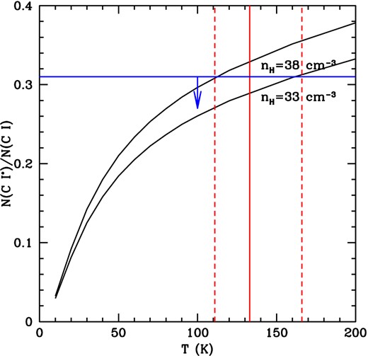
The ratio N(|${\rm C\,{\small \rm I}}$|*)/N(|${\rm C\,{\small \rm I}}$|) plotted as a function of temperature for different nH. The horizontal line shows the observed upper limit on N(|${\rm C\,{\small \rm I}}$|*)/N(|${\rm C\,{\small \rm I}}$|), while the solid and dashed vertical lines are the inferred temperature and 1σ range, respectively, for the strong H2 component.
4 CONNECTING GALAXY AND ABSORPTION PROPERTIES
The sub-DLA towards J0441−4313 is associated with a spiral galaxy at an impact parameter of ∼7.6 kpc from the QSO sightline (Petitjean et al. 1996; Chen et al. 2005). This is the lowest galaxy impact parameter at which H2 absorption has been detected at low-z (see fig. 9 of Muzahid et al. 2014), enabling the connection between absorber and galaxy properties to be well established. Chen et al. (2005) have carried out spectroscopic analysis of the galaxy, and found it to be a star-forming galaxy with an oxygen abundance more than solar ([O/H] = 0.45 ± 0.15). They derived the sub-DLA metallicity as log Z = −0.20 ± 0.30 (see Section 3.1), and hence reported a metallicity decrement along the galaxy disc. Using higher resolution data, however, we have found the average metallicity in the sub-DLA to be twice solar. Therefore, there does not appear to be any considerable metallicity gradient (−0.02 ± 0.17 dex kpc−1) along the disc of the galaxy. This is similar to the results of Péroux et al. (2012), who do not find any significant decrease between metallicity of galaxy from emission and metallicity of absorber from absorption, and even report the possibility of an increasing metallicity gradient in few cases.
Using the luminosities of the galaxy's emission lines provided by Chen et al. (2005), and the abundance determination method given in Izotov et al. (2006), we estimate [N/H] = −0.16 and hence [N/O] = −0.61 in the galaxy. Here we have assumed a typical electron temperature of 104 K. The average [N/S] ratio for the sub-DLA is −0.76 ± 0.03 (ionization corrections are negligible compared to the errors). Note that this ratio is similar within 0.1 dex across the two components. The abundances of S and O, both being α-elements, track each other. Hence, the similarity of the [N/α] ratio in both the galaxy and the sub-DLA implies that the chemical enrichment history of both are similar. Thus, the absorber may be tracing the extended neutral gas disc of the galaxy. Indeed, rotational velocity measurements of the galaxy and the sub-DLA performed by Chen et al. (2005) hints that that absorbing gas may be corotating along with the optical disc at a galactocentric radius of ∼13.6 kpc (i.e. the deprojected separation of the sub-DLA along the stellar disc). Alternatively, the gas probed by the sub-DLA could be recently ejected from the galaxy and tracing a metal-rich galactic wind/outflow.
Nitrogen can be of both primary and secondary origin, depending on whether the seed C and O are produced by the star itself during helium burning (primary), or whether they are from yields of earlier generations of stars and hence already present in the ISM from which the star formed (secondary). In nearby galaxies, it has been observed that at lower metallicities, i.e. for [O/H] ≤ 0.4, the [N/O] ratio remains constant (primary N), while it rises steeply with increasing O abundance, i.e. for [O/H] ≥ 0.7 (secondary N). Therefore, the measured [N/α] in this sub-DLA along with the high metallicity places it in the secondary regime of N production. Hence, the absorbing gas must have undergone a substantial period of star formation. This reinforces our above hypothesis of either the galaxy having an extended neutral disc out to at least ∼13 kpc or the sub-DLA tracing the metal-enriched halo gas of the galaxy. We test both these scenarios through our photoionization models in Section 5.
Another possible indication that the galaxy might have undergone recent periods of outflow is the presence of a Lyman α system at zabs = 0.10204, ∼+250 km s−1 from the sub-DLA (see fig. A2 of Muzahid et al. 2014), with Lyman α, |${\rm Si\,{\small \rm II}}$|, |${\rm Si\,{\small \rm iii}}$| and |${\rm N\,{\small \rm II}}$| transitions spread over ∼200 km s−1. We measure log N(H i)) = 14.93 ± 0.44, log N(|${\rm Si\,{\small \rm II}}$|) = 13.81 ± 0.14, log N(|${\rm Si\,{\small \rm iii}}$|) = 13.99 ± 0.19 and log N(|${\rm N\,{\small \rm II}}$|) = 14.81 ± 0.28 in this system. Based on the large metal column densities, the system could be metal rich, with metallicity and [N/α] ratio close to solar. In that case, this cloud is likely to be tracing a recent metal-enriched outflow from the galaxy. However, since only the Lyman α transition is covered for this system, the N(H i)) measurement has large uncertainties and it is plausible that the system has higher N(H i)) and lower metallicity.
5 PHOTOIONIZATION MODELS
We use the photoionization code cloudy (version 13.03; last described by Ferland et al. 2013) to model the physical conditions and infer the chemical enrichment in this system. In all our models, the absorber is considered to be a plane-parallel slab of constant density gas with the radiation field impinging on it from one side. Note that we do not aim to model all the absorbing ions detected from this system due to the multiple component nature of the absorber and complexities associated with phase structure, depletion and possible hidden saturation in the COS spectrum. We concentrate on H2, |${\rm C\,{\small \rm I}}$|, |${\rm C\,{\small \rm I}}$|* and |${\rm Na\,{\small \rm I}}$| absorption arising from Component 2, which are likely to trace the CNM and whose excitations will be governed by similar ionizing radiation. The ‘atom h2’ command of cloudy, as described in Shaw et al. (2005), is used in order to get an accurate H2 equilibrium abundance. We consider three different incident radiation fields: (i) the metagalactic UV background of QSOs and galaxies (Haardt & Madau 2012, hereafter HM12); (ii) the interstellar radiation field as in our Galaxy (Black 1987), scaled by a factor χUV and (iii) a starburst galactic radiation field. Examples of the typical incident continuum spectra for different radiation fields used in our models are shown in Fig. 3. The cosmic microwave background radiation at z = 0.1 and a cosmic ray ionization rate of log(ΓCR) = −17.3 (Williams et al. 1998) are also included. For the observed N(H i)), we find the ionization correction for the S abundance to be negligible (i.e. IC ≤−0.02) compared to the errors, for a wide range of density and radiation fields considered. Hence, the average metallicity of the system can be represented by [S/H] = 0.28 ± 0.08, i.e. Z ∼ 2 Z⊙.
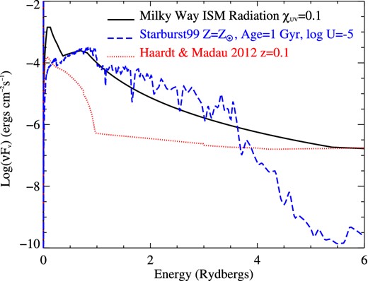
Examples of typical incident continuum spectra for different radiation fields used in our photoionization models.
In the following sections, we focus our efforts on modelling the strong H2 component (Component 2) using cloudy simulations that self-consistently compute the ion and molecular abundances along with the gas temperature. We run a grid of models by changing the density, nH (Sections 5.1 and 5.2), or the ionization parameter, U (Section 5.3), and stopping the calculations when the N(H2) in the model reaches the observed value of 1016.61 cm−2. Additionally, we discuss the effects of a high N(H2) value of 1018.9 cm−2 (see Section 3.2.1) on the models in Section 5.4. We constrain the density using the observed limit of N(|${\rm C\,{\small \rm I}}$|*)/N(|${\rm C\,{\small \rm I}}$|), the N(|${\rm C\,{\small \rm I}}$|)/N(|${\rm Na\,{\small \rm I}}$|) ratio and by requiring the N(H i)) of the model to be less than the total measured N(H i). Note that, as discussed in Section 3.1, fits to the metal lines in the COS spectrum with more than two components are not preferred. However, fitting the |${\rm C\,{\small \rm I}}$| lines with multiple components having the z and b fixed as that of the |${\rm Na\,{\small \rm I}}$| lines, allow for two times larger N(|${\rm C\,{\small \rm I}}$|) than that obtained from our best fit. We allow for this uncertainty in the column density measurements while comparing with the model predictions. Since there are many parameters in the models, for simplicity we take the metallicity in this component to be the same as the average (2 Z⊙) and the H2 formation rate, R, to be the same as that given by Jura (1975) for our Galaxy. Dust composition is assumed similar to the Galaxy and dust depletion is taken as observed for this system. The results of the models are summarized in Table 4.
Summary of the photoionization models for the strong H2 absorbing component assuming log N(H2) = 16.61 as discussed in Section 5.
| Modelsa | nH (cm−3) | |$f_{N({\rm H}\,\small {i})}$| | T (K) | log N(|${\rm C\,{\small \rm I}}$|)/N(|${\rm Na\,{\small \rm I}}$|) | log N(|${\rm C\,{\small \rm I}}$|*)/N(|${\rm C\,{\small \rm I}}$|) |
|---|---|---|---|---|---|
| HM12 TE | 0.1 | 0.5 | 160 | 2.0 | −2.3 |
| Galactic χUV = 0.1–0.5 TE | [1, 100] | [0.01, 1.0] | [20, 50] | [1.2, 1.5] | [−1.2, −0.5] |
| Galactic χUV = 0.1–0.5 CT | [3, 30] | [0.1, 1.0] | 133 | [1.1, 1.2] | [−1.3, −0.5] |
| Starburst TE | −5.5b | 0.2 | 40 | 1.6 | −0.9 |
| Starburst CT | [−5.5, −5.0]b | [0.3, 0.8] | 133 | [1.7, 1.8] | [−1.1, −1.2] |
| Observations | 133|$^{+33}_{-22}$| | 1.8 ± 0.2 | ≤−0.5 |
Notes.aTE: thermal equilibrium; CT: constant temperature.
blog (U).
5.1 Models with metagalactic UV background
We first consider the scenario in which the absorber is a gas cloud irradiated with the HM12 background. From the total N(H i)) constraint, we find that the observed N(H2) can be produced at nH ≥ 0.03 cm−3, while from the upper limit of N(|${\rm C\,{\small \rm I}}$|*)/N(|${\rm C\,{\small \rm I}}$|), we have nH ≤ 50 cm−3. For nH ∼ 0.1 cm−3, the N(|${\rm C\,{\small \rm I}}$|)/N(|${\rm Na\,{\small \rm I}}$|) ratio, N(|${\rm C\,{\small \rm I}}$|) and N(|${\rm Na\,{\small \rm I}}$|) predicted by the model is consistent with the observed values within the uncertainties. Moreover, the T01 predicted by this model is consistent with our estimation (see Table 4). Hence, just the extragalactic background can explain the observations provided the gas is at low densities. However, we note that this gas cloud is located just outside the optical disc of a star-forming galaxy (see Section 4). If we consider an incident spectrum similar to that of this galaxy and account for the measured dust extinction (see Section 5.3 for details), the expected radiation field near the absorber at 10 eV is ∼10 times higher than the HM12 background. If the |${\rm C\,{\small \rm I}}$|* absorption could be better constrained with higher resolution and S/N data or the |${\rm C\,{\small \rm II}}$|* absorption were covered, it would place additional constraint on the density, and hence allow us to test this model better. The fraction of N(H i)) associated with the H2 gas in this case is |$f_{N({\rm H\,\small {i})}} \sim 0.5$|. We estimate the size, L, of the H2 absorbing cloud, assuming spherical geometry, as ∼74 pc, using |$L = f_{N({\rm H}\,\small {i})} N({\rm H}\,\small {i}) / (f_{\rm H\,\small {i}} n_{\rm H})$|.
5.2 Models with the mean Galactic radiation field
Next, we consider the case where the absorber is situated in the extended neutral disc of a galaxy with radiation field similar to that of the Milky Way. The Galactic radiation field as given in ‘table ism’ of cloudy is the unextinguished local interstellar radiation field. However, most of the radiation field between 1 and 4 Ry is found to be heavily absorbed by gas in the ISM. Hence, using the ‘extinguish’ command of cloudy we introduce photoelectric absorption by a slab of cold neutral gas (log N(H i)) ∼ 20) to mimic typical Galactic ISM sightlines. This is a more appropriate way to model the CNM phase in the gas, since this will lead to a single neutral phase throughout the gas slab. Moreover, while the hydrogen ionizing photons emitted from the galaxy are in principle removed, the species of our interest (H2, |${\rm C\,{\small \rm I}}$|, |${\rm Na\,{\small \rm I}}$|) are susceptible to ionizing photons with energy less than 1 Ry. Note that we add the HM12 radiation field to the Galactic radiation field.
We find that when thermal equilibrium is assumed the T01 estimated by the models is too low (∼30–40 K) compared to the observed T01 (133|$^{+33}_{-22}$| K). The fact that thermal equilibrium models in cloudy produce very low T01, while using the radiation given by the ‘table ism’ in cloudy, has been noted by Srianand et al. (2014) while modelling H2 absorption in a low-z DLA. They suggested that the low temperatures in the models could be due to cloudy not considering additional non-radiative heating processes. Additional heating in DLAs can come from cosmic ray ionization (see Dutta et al. 2014). However, Srianand et al. (2014) have shown that increasing the cosmic ray ionization rate, while increasing the temperature, also causes the ion column densities to increase. Instead, they present H2 formation at lower densities through enhanced formation rate on dust grains as a possible solution for increasing the gas temperature (see also Habart et al. 2011; Le Bourlot et al. 2012).
Since the thermal equilibrium models are not able to self-consistently explain the observed temperature, we consider constant temperature models, i.e. we fix the temperature to be equal to the observed T01 throughout the gas cloud. From these models using the N(H i)) constraint and the N(|${\rm C\,{\small \rm I}}$|*)/N(|${\rm C\,{\small \rm I}}$|) limit, we find the H2 can be produced for nH ∼ 3–30 cm−3 and χUV ∼ 0.1–0.5. However, the model-predicted N(|${\rm C\,{\small \rm I}}$|)/N(|${\rm Na\,{\small \rm I}}$|) ratio for the above solution does not match the observed ratio within the allowed uncertainties (see Table 4). Hence, while the Galactic radiation field attenuated by 10–50 per cent can produce the observed N(H2), it is unlikely to produce the |${\rm C\,{\small \rm I}}$| and |${\rm Na\,{\small \rm I}}$| absorption as measured for this gas, and a weaker field may be required.
5.3 Models with starburst radiation field
Next, we consider the absorber to be present in the halo around a galaxy. Chen et al. (2005) have measured properties of the galaxy believed to be associated with this sub-DLA (see Section 4). Using their measurements, we construct a model with radiation field similar to that of the candidate host galaxy. From the Hα extinction-corrected luminosity, we estimate a star formation rate of 0.53 M⊙ yr−1 (Kennicutt 1998). Subsequently, we use starburst996 to generate the spectrum of a continuously star-forming galaxy. The metagalactic HM12 UV background is added to the above radiation field. We proceed similarly as above to estimate the physical parameters of the system, except in this case we run the model on ionization parameter grids. As in Section 5.2, the T01 estimated by this model when assuming thermal equilibrium is much lower than our measurement. Hence, we consider a model with the temperature kept constant (i.e. equal to T01). We find that such a model is consistent with our observations for −5.5 ≤ log U ≤ −5.0. This can be seen from Table 4 and Fig. 4, where we have plotted N(H i)), N(|${\rm C\,{\small \rm I}}$|*)/N(|${\rm C\,{\small \rm I}}$|), N(|${\rm C\,{\small \rm I}}$|)/N(|${\rm Na\,{\small \rm I}}$|) and column densities of |${\rm C\,{\small \rm I}}$| and |${\rm Na\,{\small \rm I}}$| obtained from the model as a function of ionization parameter. The N(|${\rm C\,{\small \rm I}}$|) and N(|${\rm Na\,{\small \rm I}}$|) are overpredicted by the model by 0.3 and 0.5 dex, respectively, which can be accounted for by depletion as seen in the Galactic CNM (Welty et al. 1999). Over the range of U where the model is consistent with our observations allowing for uncertainties in measurements and depletion effects, |$f_{N({\rm H}\,\small {i})}$| is in the range ∼0.3–0.8.
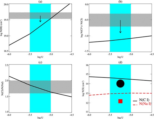
Results from photoionization model using the starburst radiation field for the strong H2 absorbing component (Section 5.3). The model-predicted N(H i)), N(|${\rm C\,{\small \rm I}}$|*)/N(|${\rm C\,{\small \rm I}}$|), N(|${\rm C\,{\small \rm I}}$|)/N(|${\rm Na\,{\small \rm I}}$|) and column densities of |${\rm C\,{\small \rm I}}$| and |${\rm Na\,{\small \rm I}}$| as a function of ionization parameter are shown in panels (a)–(d), respectively. The vertical shaded regions show the range of U in which the model is consistent with our observations. The horizontal shaded regions in (a)–(c) show the allowed range in the values from observations. The symbols circle and square in (d) show the measured N(|${\rm C\,{\small \rm I}}$|) and N(|${\rm Na\,{\small \rm I}}$|), with the size of the symbols representing the allowed uncertainties in the measurements.
We define the ionization parameter as U = QΩe− τ/(4πr2nHc), where Q is the rate at which ionizing photons are emitted by the galaxy, Ω is the solid angle subtended by the galaxy at the absorber, τ is the dust optical depth and r is the distance between the galaxy and the illuminated face of the cloud. Q can be obtained by integrating the starburst99 spectrum. Since we are estimating U using |${\rm C\,{\small \rm I}}$|, |${\rm Na\,{\small \rm I}}$| and H2 excitations, we estimate the dust optical depth at 10 eV (τ10 eV). From the extinction measurement of the galaxy, E(B − V) = 0.22 (Chen et al. 2005), the ratio of total-to-selective extinction, Rv = Av/E(B − V) = 3.1, and the Galactic extinction curve (Misselt, Clayton & Gordon 1999), we can estimate the extinction expected at 10 eV, i.e. A10 eV and hence τ10 eV. For simplicity, we approximate the galaxy as a circular disc of radius 5 kpc with uniform surface brightness, and the absorber as a point at r = 7.6 kpc along the normal to the galactic disc (Chen et al. 2005), to estimate the solid angle. Then, for the range of U obtained from the models, the expected gas density range is nH ∼ 30–90 cm−3. For the above density range and |$f_{N({\rm H}\,\small {i})}$| obtained from the models, the cloud will have size of ∼0.04–0.5 pc. We have not taken into account the angle between the absorber and the normal to the galactic disc in this simple calculation, which can cause further attenuation in the flux received by the absorber, leading to a lower density and a larger cloud size.
Hence, the absorber can be a halo cloud subject to the radiation field due to a continuously star-forming galaxy, with metallicity, star formation rate and dust extinction as seen in the candidate host galaxy. Based on the results of our photoionization models and our discussion in Section 4, we conclude that the absorber is more likely to be tracing gas ejected recently by the galaxy into the circumgalactic medium rather than originating in the extended disc. Moreover, we note that in all our photoionization model solutions, the N(|${\rm Ar\,{\small \rm I}}$|) predicted by the model is higher (by ∼0.5–1 dex) than the observed. Argon, being an inert element, is not expected to deplete on dust, and we find that |${\rm Ar\,{\small \rm I}}$| is the dominant ionization state of argon in our models. As we pointed out before, |${\rm Ar\,{\small \rm I}}$| depletion is seen in the HVCs and in some interstellar sightlines. Sofia & Jenkins (1998) have argued that this could be related to excess ionization due to hard photons. Our study suggests that for the three ionizing radiation fields considered here, Ar depletion cannot be explained by a self-consistent ionization model. Jenkins (2013) suggested that strong Ar depletion could be due to non-equilibrium ionization conditions prevailing in the absorbing gas. Alternatively, the absorber may be tracing gas that is not chemically well-mixed and that is freshly ejected into the halo from a recently exploded supernovae region in the galaxy. In order to make headway on this issue it is important to examine several species covering a wide range of ionization states using future COS observations.
5.4 Models with high |$\boldsymbol {N({\rm H}_2)}$|
In Section 3.2.1 we discussed the possibility of a high N(H2) value (1018.9 cm−2) for Component 2. However, in that case the molecular fraction will be log f(H2) = −0.57 if we consider all the N(H i)) to be associated with this component and higher otherwise. For the Galactic disc such high molecular fraction generally indicates that the N(H i)) is above the threshold (1020.7 cm−2) where the H2 molecule gets completely self-shielded from interstellar radiation (Savage et al. 1977). If we assume the H2 formation rate in this system to be same as in our Galaxy, then the high f(H2) would require either a very low photodissociation rate (i.e. a much weaker radiation field) or a very high density. We remind here that the observed T01 and fine-structure excitation of C does not allow the density to be more than few tens of H atoms cm−3 if the relevant parameters are similar to that of the Milky Way (see Section 3.2.2). To consider whether such high molecular fraction is feasible in the present system, we ran cloudy models with the three background radiation fields considered above and stopped the calculations when log N(H2) = 18.9. However, the temperature computed in all three cases is much lower (20–30 K) than the inferred T01, and hence we consider the models with constant temperature. For the extragalactic HM12 background we find that the high N(H2) can be produced for nH = 1–100 cm−3. However, the N(|${\rm C\,{\small \rm I}}$|) predicted by this model is more than 1 dex higher than the observed value. For the model with the mean Galactic radiation field, the N(H2) can be produced for nH = 10–30 cm−3 and χUV = 0.1. However, the N(|${\rm C\,{\small \rm I}}$|)/N(|${\rm Na\,{\small \rm I}}$|) ratio falls ∼1 dex below the observed value. In the case of the starburst radiation field, the N(H i)) required by the models to produce the N(H2) is higher than the total measured N(H i)) of the system. Hence, none of the radiation fields considered here is able to consistently explain the high N(H2) solution. This supports our argument that the present system is unlikely to host such high molecular fraction. However, we emphasize the need for higher S/N and higher resolution data to have better handle on the models.
6 RADIO OBSERVATIONS
6.1 VLBA mas scale imaging
This sub-DLA is unique in the sense that it is the only known low-z (i.e. z < 1.0) system with a H2 detection towards a radio-loud QSO so that 21-cm absorption observations are possible. Given the small inferred sizes from the photoionization models, mas scale VLBI imaging of the background radio source is necessary to measure the covering factor, fc, of the absorbing gas. The standard practice, in the absence of VLBI spectroscopy, is to use the ratio of the VLBI core flux density to the flux density measured in the arcsecond scale images to estimate fc (see Kanekar et al. 2009; Gupta et al. 2012; Srianand et al. 2012). We carried out continuum observations of the radio source using the VLBA. The spatial resolution achieved in our VLBA observations is ∼12 × 7 mas2, i.e. ∼23 × 13 pc2 at the redshift of the absorber. If the size of the H2 gas is of this order, then the fraction and spatial extent of the radio flux density detected in the VLBA image will determine the 21-cm absorption detectability.
The radio source is identified as a flat-spectrum radio source (Healey et al. 2007), and is unresolved at arcsecond scales with a flux density of 330 mJy at 1.29 GHz (Kanekar et al. 2001). However, most of the emission is over-resolved in our VLBA image, with only 27 per cent being recovered, assuming the continuum flux density of the radio source is constant. Our VLBA image (Fig. 5) shows an extended structure with a total flux density of 90 mJy and a peak flux density of 59 mJy beam−1. Note that we used ‘robust=2’ weighting in the aips task ‘imagr’ to obtain the image shown in Fig. 5. The largest linear size of the radio source measured from the emission detected in the VLBA image is ∼70 mas, i.e. ∼131 pc at the redshift of the absorber. From our discussion on photoionization models in the previous section, if the absorbing gas is spherical, then the expected extent of the strong H2 absorber is smaller than the extent of the radio emission seen in our VLBA image. If we associate the location of the peak emission in the VLBA image to the optical source, then the expected covering factor is ≥0.18. However, if we do not assume spherical geometry, then we do not have any constraint on the extent of the gas in the transverse direction to our line of sight. If we assume the gas to cover all the emission seen in the VLBA image, then the covering factor is 0.27. In the following section we discussion the implications of this for the detectability of 21-cm absorption.
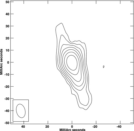
Contour plot of the VLBA image of J0441−4313 at 1.4 GHz. The rms in the image is 0.15 mJy beam−1. At the bottom of the image the restoring beam is shown as an ellipse. The beam size is 0.012 × 0.007 arcsec2. The image centre is at RA = 04h41m17|${^{\rm s}_{.}}$|3367, Dec. = −43°13′45|${^{\prime\prime}_{.}}$|4394. The contour levels are plotted as 0.46 × (−2,−1, 1, 2, 4, 8,...) mJy beam−1.
6.2 21-cm absorption
In the ATCA radio spectrum (with a channel resolution of 1.8 km s−1) reported by Kanekar et al. (2001), no 21-cm absorption is seen at the zabs of Component 2 at the level of 1.56 mJy (the spectral rms), while a line is tentatively detected at 3.3σ at zabs = 0.10097 in a spectrum smoothed to 9 km s−1. The 21-cm optical depth τ21 is related to the N(H i)) (cm−2) and Ts (K) as N(H i)) = 1.823 × 10¹⁸ (Ts/fc)∫τ21 dv, where the H i 21-cm line is assumed to be optically thin. In the galactic ISM, the kinetic temperature measured from H2 usually follows the H i spin temperature (Roy et al. 2006). We assume this to hold for the present system as well. If all the N(H i)) were associated with Component 2, we would expect a ∼3 mJy line, assuming fc = 0.27 and a line width of 5 km s−1, which is ruled out at 2σ. Hence, the H2 gas cannot have all the N(H i)) associated with it and cover all the radio emission in the VLBA image. However, if the H2 gas were to have ≤50 per cent of the total N(H i)) or cover only part the VLBA emission, the present spectrum would not be sensitive enough to detect 21-cm absorption from this gas. A factor of 3 higher S/N spectrum will allow us to detect or constrain the 21-cm absorption at a significance of 3σ.
The weak 3.3σ 21-cm detection lies within ∼15 km s−1 of the weaker H2 component, and ∼8 km s−1 of the weaker components of |${\rm C\,{\small \rm I}}$|, |${\rm Ca\,{\small \rm II}}$| and |${\rm Na\,{\small \rm I}}$|. Recall that the measured column densities of metals and dust depletion in this component are not very different from that of the strong H2 component. Usually the absence/weakness of H2 and |${\rm C\,{\small \rm I}}$| is ascribed to high temperatures and low densities (Srianand et al. 2005). In this case we know that the temperature cannot be very high, since the H2, |${\rm C\,{\small \rm I}}$|, |${\rm Na\,{\small \rm I}}$| absorption are weak, and the ratio of column densities of the J = 0 and 1 levels of H2 in this component suggests that the temperature is ≥100 K. If we consider the optical depth reported by Kanekar et al. (2001), and assume fc = 0.27 and all of the N(H i)) to be associated with the weak H2 component, then Ts will be ∼90 K. However, from the observed metal content across the components and our photoionization models, the weaker component is not likely to have all the N(H i)) associated with it. For |$f_{N({\rm H}\,\small {i})}$| = 0.5 and fc = 0.27, the Ts will be ∼45 K. In case the covering factor is lower than 0.27, the inferred Ts will be even lower. It will be surprising to have such a low temperature in a gas with N(H i)) ∼ few 1019 cm−3. It is most likely that one will need higher densities and a lower radiation field. In that case it will be interesting to ask why |${\rm C\,{\small \rm I}}$| lines are weak in such a cold and dense gas. The discussions presented in this section clearly bring out the importance of having a much higher S/N spectrum to confirm the 21-cm detection reported by Kanekar et al. (2001), and have a stronger constraint on the absence of 21-cm absorption in the strong H2 component. In addition, better constraints on the |${\rm C\,{\small \rm I}}$|* and |${\rm C\,{\small \rm II}}$|* absorption will allow us to learn more about the physical conditions of the cold gas in this interesting absorber.
7 SUMMARY
We have carried out a detailed analysis of the cold gas phase in the sub-DLA at zabs = 0.10115 towards J0441−4313, in which H2 absorption has been detected by Muzahid et al. (2014). This unique system allows us to study the physical conditions in the absorbing gas using both H2 and 21-cm absorption simultaneously for the first time at z < 1. Below we summarize the main results of our study.
The H2 absorption arises from one strong component at zabs = 0.10115, with log N(H2) = 16.61 ± 0.05, along with another weaker component at zabs = 0.10091, with log N(H2) ≤ 15.51 ± 0.03. We note that the N(H2) measurement of the strong H2 component is uncertain due the medium resolution of the COS spectrum, and that the N(H2), in principle, can be much higher if the actual b parameter is much smaller. However, the absence of H2 absorption from higher J levels and of HD absorption, as well as our photoionization modelling, do not seem to support a high N(H2). The excitation temperature (133|$^{+33}_{-22}$| K) measured in the strong component for the range log N(H2) = 16.6–18.9 is similar to what is expected from a CNM phase.
The average metallicity of the absorber is found to be twice solar and the dust depletion moderate ([Fe/S] ∼ −0.49). We do not find any significant variation in depletion across the two metal components detected in the COS spectrum. The strong H2 component accounts for 55–65 per cent of the metal column densities. Interestingly, the stronger components of |${\rm C\,{\small \rm I}}$|, |${\rm Na\,{\small \rm I}}$| and |${\rm Ar\,{\small \rm I}}$| are coincident with this component.
The sub-DLA is known to be associated with a star-forming galaxy at a projected separation of ∼7.6 kpc, just outside the optical galactic disc (Chen et al. 2005). We do not find any metallicity gradient between the host galaxy and the sub-DLA as suggested by Chen et al. (2005). Moreover, the [N/α] ratio measured in both are similar. Hence, the galaxy is likely to either have a metal-rich neutral disc extending to at least ∼13 kpc (the galactocentric radius of the sub-DLA) or have undergone recent periods of metal-rich outflow.
From photoionization modelling, we show that the observed column densities of H2, |${\rm C\,{\small \rm I}}$| and |${\rm Na\,{\small \rm I}}$| in the zabs = 0.10115 component can be consistently explained using a radiation field due to a continuously star-forming galaxy, with metallicity, star formation rate and dust extinction as measured in the associated galaxy. Alternatively, if the absorber is tracing the extended galactic disc, then the radiation field has to be weaker than half the mean Galactic radiation field. However, the models suggest that the absorber is more likely to be tracing gas in the galactic halo than in the extended galactic disc. We note that the measured column densities are also consistent with the extragalactic background radiation if the gas has nH ∼ 0.1 cm−3 and L ∼70 pc. However, from the presence of a star-forming galaxy at ∼7.6 kpc, we argue that this absorber is more likely to be a halo cloud. In that case, using simple approximations we obtain for this gas cloud, nH ∼ 30–90 cm−3 and L ∼ 0.05–0.4 pc.
The measured |${\rm Ar\,{\small \rm I}}$| absorption strength in this system is much weaker than what is expected if there is no depletion or ionization effects, and than what is predicted by all our photoionization models. Similar depletion is seen in the case of HVCs in our Galaxy. The possible explanations could be non-equilibrium ionization conditions in the absorber or the gas not being chemically well mixed due to recent ejection from supernovae region in the associated galaxy.
This sub-DLA presents a fortuitous case of a H2 absorber towards a radio-loud QSO which can be searched for 21-cm absorption. We present the VLBA mas scale image of the background radio source, which shows it to be over-resolved, with only 27 per cent of the arcsecond flux being recovered. The radio emission has a total flux density of 90 mJy, a peak flux density of 59 mJy beam−1 and an extent of ∼131 pc at the redshift of the absorber.
Kanekar et al. (2001) report a tentative detection of weak 21-cm absorption that arises within ∼15 km s−1 of the weaker H2 component. However, 21-cm absorption from the stronger H2 component is absent at the level of 2σ, indicating that either the N(H i)) associated with this component is ≤50 per cent of the total measured N(H i)) or that the covering factor of this gas is ≤0.27, consistent with results from our photoionization models.
The reported 21-cm absorption from the weaker H2 component indicates that Ts ≤ 90 K in this gas. The actual value could be much lower if a good fraction of the observed N(H i)) is associated with the strong H2 component. However, the weakness of H2, |${\rm C\,{\small \rm I}}$| and |${\rm Na\,{\small \rm I}}$| absorption from such cold gas is puzzling. A higher S/N 21-cm absorption spectrum and a UV spectrum with better coverage of species like |${\rm C\,{\small \rm I}}$|, |${\rm C\,{\small \rm I}}$|* and |${\rm C\,{\small \rm II}}$|* are essential to put more stringent constraints on the conditions in this absorbing gas.
Such detailed analysis of similar individual systems is essential to further our understanding of the properties of cold gas present around galaxies, and in particular, of the connection between H2 and 21-cm absorption. The results presented here will also facilitate interpretation of the results of large surveys of H2 and 21-cm absorption.
We thank the anonymous referee for useful comments. The VLBA is run by the National Radio Astronomy Observatory. The National Radio Astronomy Observatory is a facility of the National Science Foundation operated under cooperative agreement by Associated Universities, Inc. This work made use of the Swinburne University of Technology software correlator, developed as part of the Australian Major National Research Facilities Program and operated under license (Deller et al. 2011).
Based on observations made with the NASA/ESA Hubble Space Telescope, obtained from the data archive at the Space Telescope Science Institute, which is operated by the Association of Universities for Research in Astronomy, Inc., under NASA contract NAS 5-26555; data obtained from the ESO Science Archive Facility under request number rdutta129485; data obtained with Very Long Baseline Array (Prgrm. ID: BD187, PI: Dutta).
Here, |$N({\rm Fe}_{\rm dust}) = N(\rm S)[ 1\hbox{-}10^{[\rm Fe/S]}](\rm Fe/S)_{{\odot }}$| and |$\kappa = 10^{[\rm S/H]} [ 1\hbox{-}10^{[\rm Fe/S]}]$|.
f(H2) = 2N(H2)/(2N(H2) + N(H i))).
