On properties of Velikhov–Chandrasekhar MRI in ideal and non-ideal plasma

Abstract

1 INTRODUCTION

In the end of the 1950s – beginning of the 1960s, E. Velikhov and S. Chandrasekhar studied the stability of sheared hydromagnetic flows (Velikhov 1959; Chandrasekhar 1960). In these papers, the magnetorotational instability (MRI) in axisymmetric flows with magnetic field was discovered. MRI arises when a relatively small seed poloidal magnetic field is present in the fluid. This instability was applied to astrophysical accretion discs in the influential paper by Balbus & Hawley (1991), and since then has been considered as the major reason for the turbulence arising in accretion discs (see Balbus & Hawley 1998 for a review). Non-linear numerical simulations (e.g. Hawley, Gammie & Balbus 1995; Sorathia et al. 2012; Hawley et al. 2013) confirmed that MRI can sustain turbulence and dynamo in accretion discs. However, semi-analytical and numerical simulations (see for example, Masada & Sano 2008; Stone 2011; Hawley et al. 2013; Nauman & Blackman 2015; Suzuki & Inutsuka 2014) suggest that the total (Reynolds + Maxwell) stresses due to MRI are insufficient to cause the effective angular momentum transfer in accretion discs in terms of the phenomenological alpha-parameter α_SS (Shakura & Sunyaev 1973), giving rather low values α_SS ∼ 0.01–0.03. Note that from the observational point of view, the alpha-parameter can be reliably evaluated, e.g. from the analysis of non-stationary accretion discs in X-ray novae (Suleimanov, Lipunova & Shakura 2008), dwarf-nova and AM CVn stars (Kotko & Lasota 2012), and turns out to be an order of magnitude higher than typically found in the numerical MRI simulations.

In this paper, we use the local linear analysis of MRI in the WKB-approximation by Balbus & Hawley (1991) to examine properties of MRI for different laws of differential rotation in weakly magnetized flows, Ω²(r) ∝ r⁻ⁿ, i.e. when the solution to linearized magnetohydrodynamic (MHD) equations in the Boussinesq approximation is searched for in the form |$\sim {\rm e}^{{\rm i}(\omega t-k_r r-k_z z)}$|⁠, where k_r, k_z are wave vectors in the radial and normal direction to the disc plane, respectively, in the cylindrical coordinates.

In this approximation, the dispersion relation represents a biquadratic algebraic equation. The linear local analysis of unstable modes in this case was performed earlier (see e.g. Balbus 2012). Here, we emphasize the different behaviour of stable and unstable modes of this equation for different rotation laws of the fluid. We show that in the Rayleigh-unstable hydrodynamic case where the angular momentum decreases with radius, the Velikhov–Chandrasekhar MRI does not arise, and the magnetic field suppresses the Rayleigh instability at small wavelengths.

Then, we turn to the analysis of non-ideal plasma characterized by non-zero kinematic viscosity ν and magnetic diffusivity η. This problem has been addressed previously by different authors (see e.g. Balbus & Hawley 1998; Sano & Miyama 1999; Ji, Goodman & Kageyama 2001; Balbus 2004; Islam & Balbus 2005; Pessah & Chan 2008, among others), aimed at studying various aspects of the MRI physics and applications. To keep the paper self-contained, we re-derive the basic dispersion relation in the general case and investigate its behaviour for different values of the magnetic Prandtl number P_m = ν/η and the kinematic vicosity ν. Specifically, we consider the limitations implied by the viscosity in accretion discs with finite thickness, and find phenomenologically interesting constraints on the disc parameters where MRI can operate.

The structure of the paper is as follows. In Section 2, we repeat the linear WKB analysis for small perturbations in an ideal fluid and consider five different cases for MRI and Rayleigh modes. We also investigate the behaviour of MRI at vanishing magnetic field. In Section 3, we generalize the linear analysis for non-ideal plasma with non-zero viscosity and magnetic diffusion. First, we analytically investigate the growth of linear perturbations in a plasma with the Prandtl number P_m = 1, and then consider the case of a plasma with arbitrary Prandtl number and viscosity. We discuss the results in Section 4. In Appendix A, we delineate the derivation of the dispersion equation for non-ideal plasma in the Boussinesq approximation for both adiabatic and non-adiabatic perturbations, and in Appendix B we find the analytical solution of this dispersion equation for Keplerian discs at the neutral point.

2 LINEAR ANALYSIS FOR IDEAL FLUID

According to the classical Rayleigh criterion (Lord Rayleigh 1916), if the epicyclic frequency κ² > 0 (in this case the angular momentum in the flow increases with radius), the equilibrium is stable. If κ² < 0 (the angular momentum decreases with radius), the equilibrium is unstable. If κ² = 0 (the angular momentum does not change with radius), the equilibrium is indifferent.

2.1 Ideal MHD case

Let us start with discussing the behaviour of different modes of dispersion relation (1) in the ideal MHD case. It is instructive to investigate the asymptotics of these modes with decreasing (but non-zero) seed magnetic field (see Section 2.2 for more detail on the limiting transition for vanishing magnetic field).

If the magnetic field is present, there are five different types of solutions of equation (5) depending on how the angular velocity (angular momentum) changes with radius.

Case 1: κ² > 4Ω², n < 0. In this case, there are two stable modes (see Fig. 1), which at large k² (short-wavelength limit) tend to the asymptotic behaviour |$\omega ^2=(k_z/k)^2c_{\rm A}^2k^2$|⁠. With decreasing (but non-zero) seed magnetic field amplitude B₀ (and the corresponding unperturbed Alfvén velocity c_A), one mode tends to the classical Rayleigh branch |$\omega _{\rm R}^2=(k_z/k)^2\kappa ^2$| (the horizontal dashed line in Fig. 1), and the second mode tends to the neutral branch |$\omega _{{\rm VC}}^2\rightarrow 0$|⁠.

Figure 1.

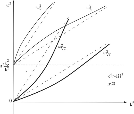
Schematic behaviour of two branches of dispersion equation (1) (‘Reynolds mode’ |$\omega _{\rm R}^2$|⁠, thin curves, and ‘MRI mode’ |$\omega _{{\rm VC}}^2$|⁠, thick curves) for two values of the Alfvén velocity |$c_{\rm A}^2$| (two values of the seed magnetic field B₀). The dashed straight lines show the asymptotic behaviour of the solutions at large k|$\omega^2=(k_z/k)^2c_\mathrm{A}^2k^2$|⁠. The smaller the seed magnetic field, the smaller the slope of the asymptotes. Case 1 of the angular velocity and angular momentum increasing with radius (κ² > 4Ω²; n < 0).

Open in new tabDownload slide

Figure 2.

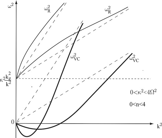
The same as in Fig. 1 for the case of decreasing angular velocity with radius but increasing angular momentum (0 < κ² < 4Ω²; 0 < n < 4) (case 2).

Open in new tabDownload slide

Case 3: κ² = 0, n = 4. In this case (see Fig. 3), both the Rayleigh mode |$\omega _{\rm R}^2$| and the MRI mode |$\omega _{{\rm VC}}^2$| go out of zero with infinite derivatives (positive and negative for the Rayleigh and MRI modes, respectively). With finite seed magnetic field, the |$\omega _{{\rm VC}}^2$| mode displays the MRI. As B₀ becomes small (but non-zero), both modes asymptotically approach the neutral mode ω² → 0.

Figure 3.

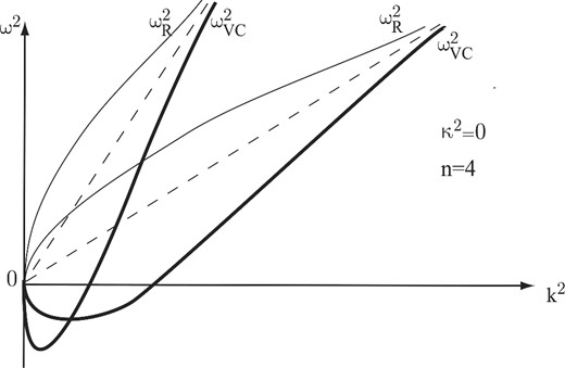
The same as in Fig. 1 for the case of constant angular momentum (κ² = 0; n = 4) (case 3). Both the Rayleigh and MRI branches have infinite derivatives dω²/dk² at k² = 0.

Open in new tabDownload slide

Case 4: κ² < 0, 4 < n < 8. In this case (see Fig. 4) in the absence of magnetic field, the instability according to the Rayleigh criterion takes place (the bottom dashed horizontal line in Fig. 4) with |$\omega _{\rm R}^2=\kappa ^2 (k_z/k)^2$|⁠. If the magnetic field is present, the Rayleigh instability is stabilized by the magnetic field at |$k^2>k^2_{{\rm cr}}$| (bottom thin curves in Fig. 4). Note that |$k_{{\rm cr}}^2$| and |$k_{{\rm max}}^2$| here are the same as in Case 2. While similar to the MRI mode, this is now the Rayleigh mode|$\omega _{\rm R}^2$| that is unstable and reaches maximum growth rate |$\omega _{{\rm R},{\rm max}}^2$| determined by equation (8). In contrast, the Velikhov–Chandrasekhar mode|$\omega _{{\rm VC}}^2$| (upper thick curves in Fig. 4) remains stable at all wavenumbers, and with decreasing (but non-zero) magnetic field |$\omega _{{\rm VC}}^2\rightarrow +0$|⁠. We stress again that the difference between the Rayleigh and MRI modes is due to their different asymptotic behaviour as B₀ → +0: the Rayleigh mode is unstable and behaves as |$\omega _{\rm R}\rightarrow -\kappa ^2 k_z^2/k^2$|⁠, unlike the stable Velikhov– Chandrasekhar mode.

Figure 4.

The same as in Fig. 1 for the case of decreasing angular momentum (κ² < 0; 4 < n < 8) (Case 4). Instability according to the Rayleigh criterion occurs. The Rayleigh branch has a negative derivative at k² = 0.

Open in new tabDownload slide

Case 5: κ² < 0, n > 8. The only difference of this case from Case 4 is that the Rayleigh mode |$\omega _{\rm R}^2$| goes out of zero with a positive derivative (bottom thin curves in Fig. 5).

Figure 5.

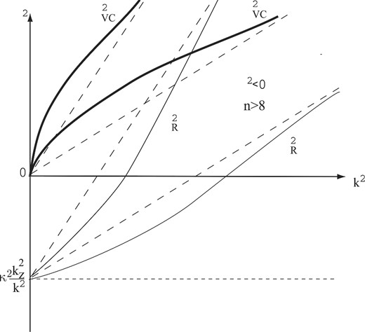
The same as in Fig. 4 for the case (κ² < 0; n > 8) (case 5 in the text); the Rayleigh branch has a positive derivative at k² = 0.

Open in new tabDownload slide

2.2 On the behaviour of MRI at vanishing magnetic field

Similarly, no smooth transition to the hydrodynamic case occurs if viscosity is included (see below). The absence of the smooth transition to the ideal hydrodynamic case when B → 0 was first noted by Velikhov (1959). At the same time, the transition to the classical Rayleigh mode with vanishing magnetic field occurs smoothly.

3 LINEAR ANALYSIS FOR FLUID WITH VISCOSITY AND MAGNETIC DIFFUSIVITY

As was shown by Balbus & Henri (2008), the magnetic Prandtl number can be of the order of one in the inner parts of accretion discs around neutron stars and black holes.

3.1 The case of the magnetic Prandtl number P_m = 1

Here, we will discuss the exact analytic solution to equation (13) for the important particular case P_m = 1 (which can be derived, for example, from the general analytic solution found in Pessah & Chan 2008) and obtain restrictions on the maximum mean-free path length of ions in accretion discs at which MRI disappears due to non-ideality effects.

Figure 6.

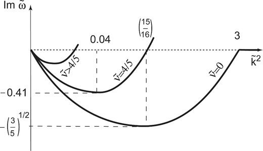
Schematics of the influence of viscosity on the MRI condition |$0<\tilde{k}<\tilde{k}_{{\rm cr}}$|⁠. Shown are curves of the imaginary part of |$\tilde{\omega }$| as a function of the dimensionless wavenumber |$\tilde{k}^2$|⁠. With increasing viscosity, the MRI interval shifts to the left and shrink (see also fig. 1 in Pessah & Chen 2008).

Open in new tabDownload slide

3.2 The case of arbitrary magnetic Prandtl number

Figure 7.

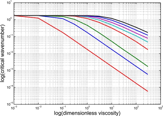
Dimensionless critical wavenumber |$\tilde{k}_{{\rm cr}}$| as a function of dimensionless viscosity coefficient |$\tilde{\nu }$| for different magnetic Prandtl numbers P_m. Lines from bottom to top correspond to P_m = 0.01, 0.1, 0.3, 3, 10, 30, 100, 300.

Open in new tabDownload slide

4 DISCUSSION AND CONCLUSION

In this paper, we have extended the original analysis of MRI in ideal MHD plasmas carried out by Balbus (2012). First, we emphasize that hydromagnetic flows in which the angular momentum increases or decreases with radius are different from the point of view of the MRI development. In the classical Rayleigh-unstable case where the angular momentum decreases with radius, the Velikhov–Chandrasekhar MRI mode is stable, while the Rayleigh mode is unstable (see Figs 4 and 5); the magnetic field stabilizes the Rayleigh mode in the short-wavelength limit. When the angular momentum in the flow increases with radius, MRI arises at long wavelengths (small wave numbers k, see Fig. 2). However, the local WKB-approximation should be applied with caution at long wavelengths. At long wavelengths, the ansatz for the solution should be rather taken in the global form |$f(r){\rm e}^{{\rm i}(\omega t-k_rr-k_zz)}$|⁠. Note that the original papers by Velikhov and Chandrasekhar analysed the linear stability of magnetized flows between cylinders exactly in that approximation (see also Sano & Miyama 1999 for the global analysis of perturbations in an inviscid magnetized protoplanetary discs with non-zero magnetic diffusivity).

Secondly, in the phenomenologically interesting case of thin Keplerian accretion discs, viscosity may restrict MRI growth. This situation can be realized in the inner parts of accretion discs. Indeed, at high temperatures the mean-free path of ions l ∼ T² can become comparable with the characteristic disc thickness H at H < r (thin discs). This means that the flow should be treated kinetically [see for example, recent 2.5D hybrid calculations (Shirakawa & Hoshino 2014) or the discussion of MRI in rarefied astrophysical plasmas with Braginskii viscosity in Islam & Balbus 2005. The seed small magnetic field under these conditions does not grow, i.e. the high ion viscosity can suppress MRI. Clearly, this interesting regime requires further study.

At large magnetic Prandtl numbers P_m ≫ 1, which can be realized in the innermost parts of accretion discs around neutron stars and black holes, the kinematic viscosity ν is much larger than the magnetic diffusivity η. In this case, plasma may become collisionless, and hydrodynamic description fails. Our analysis shows that in principle the collisionless regime (the ion mean-free path comparable to or larger than the disc thickness, l ∼ H) in Keplerian discs can be realized even for magnetic Prandtl numbers P_m ≃ 1 (see equation 39).

We have also obtained the dispersion relation for local small perturbations in the Boussinesq limit for non-adiabatic perturbations (see equation A32). This is the fifth-order algebraic equation, in contrast to the fourth-order dispersion relation for adiabatic perturbations or non-adiabatic perturbations with k_r = 0 in non-ideal plasma (equation 13). Also note that when the density perturbations are expressed through the entropy gradients (see equation 2.2 h in Balbus & Hawley 1991), the frequency appears in the denominator but the final dispersion relation (2.5) in Balbus & Hawley (1991) remains to be the fourth-order equation in ω even with taking into account the entropy gradients. Apparently, the difference is due to the fact that in the case of non-adiabatic perturbations the density variations are proportional to the azimuthal velocity perturbations u_ϕ (see our equation A21) and not to u_z and u_r as in the case considered by Balbus & Hawley (1991). The analysis of the effect of non-adiabatic perturbations deserves a separate study and will be addressed in a future work.

We conclude that in thin Keplerian accretion discs the adding of viscosity can strongly restrict the MRI conditions once the mean-free path of ions becomes comparable with the disc thickness. These limitations should be taken into account in the direct numerical simulations of MRI in astrophysical accretion discs.

We thank the anonymous referee for drawing our attention to earlier papers by Pessah & Chan (2008), Islam & Balbus (2005) and Masada & Sano (2008) and for the constructive criticism. We also thank Professor Dr. F. Meyer for discussions and MPA (Garching) for hospitality. The work was supported by the Russian Science Foundation grant 14-12-00146.

REFERENCES

APPENDIX A: DERIVATION OF THE DISPERSION EQUATION FOR NON-IDEAL PLASMA

Here, we generalize the derivation of the MRI dispersion equation (1) given in Kato et al. (1998) for the case of non-ideal plasma with arbitrary kinetic coefficients ν and η (see also Ji et al. 2001).

The system of non-deal MHD equations reads

1. mass conservation equation

   \begin{equation} \frac{\mathrm{\partial} \rho }{\mathrm{\partial} t}+\nabla \cdot (\rho \boldsymbol {u})=0\,, \end{equation}

   (A1)
2. Navier–Stokes equation including gravity force and Lorentz force

   \begin{eqnarray} \frac{\mathrm{\partial} \boldsymbol {u}}{\mathrm{\partial} t}+(\boldsymbol {u}\nabla )\cdot \boldsymbol {u}=-\frac{1}{\rho }\nabla p - \nabla \phi _{\rm g} + \frac{1}{4\pi \rho }(\nabla \times \boldsymbol {B})\times \boldsymbol {B}+\nu \Delta \boldsymbol {u} \nonumber\\ \end{eqnarray}

   (A2)

   (here ϕ_g is the Newtonian gravitational potential)
3. induction equation

   \begin{equation} \frac{\mathrm{\partial} \boldsymbol {B}}{\mathrm{\partial} t}=\nabla \times (\boldsymbol {u}\times \boldsymbol {B})+\eta \Delta \boldsymbol {B}\,, \end{equation}

   (A3)
4. energy equation

   \begin{equation} \frac{\rho {\cal R} T}{\mu }\left[ \frac{\mathrm{\partial} s}{\mathrm{\partial} t}+(\boldsymbol {u}\nabla )\cdot s \right]= Q_{{\rm visc}}-\nabla \cdot \boldsymbol {F}+\frac{\eta }{4\pi }[\nabla \times \boldsymbol {B}]^2\,, \end{equation}

   (A4)

   where s is the specific entropy (per particle), |${\cal R}$| is the universal gas constant, μ is the molecular weight, T is the temperature, and terms on the right stand for viscous, energy flux |$\boldsymbol {F}$| and Joule dissipation, respectively.
5. These equations should be completed with the equation of state for a perfect gas, which is convenient to write in the form

   \begin{equation} p=K{\rm e}^{s/c_{\rm V}}\rho ^\gamma\!, \end{equation}

   (A5)

   where K is a constant, c_V is the specific volume heat capacity and γ = c_p/c_V is the adiabatic index (5/3 for the monoatomic gas).

We will consider small axially symmetric perturbations in the WKB-approximation with space–time dependence |${\rm e}^{{\rm i}(\omega t-k_r r-k_z z)}$|⁠, where r, z, ϕ are cylindrical coordinates. The unperturbed magnetic field is assumed to be purely poloidal: |${\boldsymbol {B}_0}=(0, 0, B_0)$|⁠. The velocity and magnetic field perturbations are |$\boldsymbol {u}=(u_r,u_\phi ,u_z)$| and |$\boldsymbol {b}=(b_r, b_\phi , b_z)$|⁠, respectively. The density, pressure and entropy perturbations are ρ₁, p₁, and s₁ over the unperturbed values ρ₀, p₀, and s₀, respectively. To filter out magnetoacoustic oscillations arising from the restoring pressure force, we will use the Boussinesq approximation, i.e. consider incompressible gas motion |$\nabla \cdot \boldsymbol {u}=0$|⁠. In the energy equation, we neglect Eulerian pressure variations, p₁(t, r, ϕ, z) = 0, but Lagrangian pressure variations δp(t, r(t₀), ϕ(t₀, z(t₀)) are non-zero. (We remind that for infinitesimally small shifts the perturbed gas parcel acquires the pressure equal to that of the ambient medium; see e.g. Spiegel & Veronis 1960; Kundu, Cohen & Dowling 2012 for discussion of the Boussinesq approximation).

In the linear approximation, the system of differential non-ideal MHD equations is reduced to the following system of algebraic equations.

• The Boussinesq approximation for gas velocity |$\boldsymbol {u}$| is |$\nabla \cdot \boldsymbol {u}=0$|⁠:

  \begin{equation} k_r u_r+k_zu_z=0\,. \end{equation}

  (A6)
• The radial, azimuthal and vertical components of the Euler momentum equation are, respectively:

  \begin{eqnarray} \mathrm{i}\omega u_r-2\Omega u_\phi =\mathrm{i}k_r\frac{p_1}{\rho _0}-\frac{\rho _1}{\rho _0^2}\frac{\mathrm{\partial} p_0}{\mathrm{\partial} r}+\mathrm{i}\frac{c_{\rm A}^2}{B_0}(k_rb_z-k_zb_r)-\nu k^2u_r, \nonumber\\ \end{eqnarray}

  (A7)
  \begin{equation} \mathrm{i}\omega u_\phi +\frac{\kappa ^2}{2\Omega }u_r=-\mathrm{i}\frac{c_{\rm A}^2}{B_0}k_zb_\phi -\nu k^2u_\phi \,, \end{equation}

  (A8)

  \begin{equation} \mathrm{i}\omega u_z=\mathrm{i}k_z\frac{p_1}{\rho _0}-\frac{\rho _1}{\rho _0^2}\frac{\mathrm{\partial} p_0}{\mathrm{\partial} z}-\nu k^2u_z. \end{equation}

  (A9)

  Here, |$k^2=k_r^2+k_z^2$| so that in the linear order |$\nu \Delta \boldsymbol {u}\rightarrow -\nu k^2\lbrace u_r,u_\phi ,u_z\rbrace$|⁠,² and we have introduced the unperturbed Alfvén velocity |$c_{\rm A}^2=B_0^2/(4\pi \rho _0)$|⁠.

APPENDIX B: ANALYTICAL SOLUTION FOR THE CRITICAL WAVENUMBER |$\tilde{k}_{{\rm cr}}$| IN THE GENERAL CASE OF NON-IDEAL PLASMA