


Abstract
We study the impact of different discretization choices on the accuracy of smoothed particle hydrodynamics (SPH) and we explore them in a large number of Newtonian and special-relativistic benchmark tests. As a first improvement, we explore a gradient prescription that requires the (analytical) inversion of a small matrix. For a regular particle distribution, this improves gradient accuracies by approximately 10 orders of magnitude and the SPH formulations with this gradient outperform the standard approach in all benchmark tests. Secondly, we demonstrate that a simple change of the kernel function can substantially increase the accuracy of an SPH scheme. While the ‘standard’ cubic spline kernel generally performs poorly, the best overall performance is found for a high-order Wendland kernel which allows for only very little velocity noise and enforces a very regular particle distribution, even in highly dynamical tests. Thirdly, we explore new SPH volume elements that enhance the treatment of fluid instabilities and, last, but not least, we design new dissipation triggers. They switch on near shocks and in regions where the flow – without dissipation – starts to become noisy. The resulting new SPH formulation yields excellent results even in challenging tests where standard techniques fail completely.
1 INTRODUCTION
Smoothed particle hydrodynamics (SPH) is a completely mesh-free, fully conservative hydrodynamics method originally suggested by Lucy (1977) and Gingold & Monaghan (1977) in an astrophysical context. By now, SPH has spread far beyond its original scope and it has also found a multitude of applications in engineering. For detailed overviews over the various aspects of the method and its applications, the interested reader is referred to recent SPH reviews (Monaghan 2005; Rosswog 2009; Springel 2010a; Monaghan 2012; Price 2012; Rosswog 2014).
SPH has long been appreciated for a number of properties that are highly desirable in an astrophysical simulation. One of them is SPH's natural adaptivity that comes without the burden of additional infrastructure such as an adaptive mesh. SPH is not constrained by any prescribed geometry (as is usually the case in Eulerian approaches), the SPH particles simply follow the gas flow. SPH naturally has tendency to ‘refine on density’ and therefore vacuum is modelled with ease: it is simply devoid of SPH particles and no computational resources are wasted for modelling it. In Eulerian approaches, vacuum usually needs to be modelled as a low-density fluid and the interaction of the ‘real’ fluid with the background medium can introduce substantial artefacts such as spurious friction or shocks which need to be disentangled from the physical results.
The probably most salient advantage of SPH, however, is that the conservation of mass, energy, momentum and angular momentum can be ‘hardwired’ into discrete SPH formulations so that conservation is guaranteed independent of the numerical resolution. In practice, this conservation is only limited by, say, time integration accuracy or the accuracy with which gravitational forces are calculated. These issues, however, are fully controllable and can be adjusted to the desired accuracy. The exact conservation is usually enforced via symmetries in the SPH particle labels together with gradients that are antisymmetric with respect to the exchange of two particles. In SPH, this is usually ensured by the use of radial kernels, |$W(\boldsymbol {r})= W(|\boldsymbol {r}|)$|, and the application of direct kernel gradients with the property |$\nabla _a W(|\boldsymbol {r}_a - \boldsymbol {r}_b|) = - \nabla _b W(|\boldsymbol {r}_a - \boldsymbol {r}_b|)$|. See, for example, section 2.4 in Rosswog (2009) for detailed discussion of conservation in SPH. Below, we will also discuss an alternative gradient estimate that shares the same antisymmetry properties.
Another, highly desirable property is Galilean invariance. For an Eulerian approach, it is crucial to perform a simulation in the best possible reference frame. For example, a binary system modelled in a space-fixed frame may completely spuriously spiral in and merge while the same simulation performed in the frame of the binary system would have delivered the correct, stable orbital revolution (New & Tohline 1997). For further examples related with Galilean invariance, see Springel (2010b). Closely related is SPH's perfect advection property: a property assigned to an SPH particle, say a nuclear composition, is simply (and exactly) carried along as the particle moves. This is highly desirable in a number of contexts, for example, when fluid trajectories need to be post-processed with nuclear reaction networks.
But as every numerical method, SPH has also properties where improvements would be welcome and this is the topic of this paper. Most SPH codes use artificial viscosity to ensure the Rankine–Hugoniot relations in shocks. Often, artificial viscosity is considered a drawback, but a well-designed artificial dissipation scheme should perform similar to an approximate Riemann solver. The major challenge in this respect is to design switches that apply dissipation only where needed and not elsewhere. We discuss such switches in detail in Section 6.3. Another drawback of standard SPH approaches that has received much attention in recent years is that, depending on the numerical setup, at contact discontinuities spurious surface tension forces can emerge that can suppress subtle fluid instabilities (Agertz et al. 2007; Read, Hayfield & Agertz 2010; Springel 2010a). The reason for these surface tension forces is a mismatch in the smoothness of the internal energy and the density. This observation also provides strategies to cure the problem, either by smoothing the internal energies via artificial conductivity (Price 2008) or by reformulating SPH in terms of volume elements that differ from the usual choice m/ρ (Saitoh & Makino 2013; Hopkins 2013). Such approaches are discussed in detail and generalized to the special-relativistic case in Section 5.
SPH as derived from a Lagrangian has a built-in ‘re-meshing’ mechanism: while the particles follow the fluid flow, they try to arrange themselves into optimal relative positions that maximize the sum of the particle volumes. In other words, the SPH force is a sum of a regularization term and the approximation to the hydrodynamic force. For optimally distributed particles, the first term vanishes and the second one becomes identical to the Euler momentum equation. If the particles are, however, arranged in a non-optimal way, they start to move to improve the local distribution and this will appear as noise. Such motion is unavoidable, for example, in a multidimensional shock where the particles have to transition from the pre- to the post-shock lattice. While this re-meshing mechanism is highly desirable, the related motions should be very subtle. This can be achieved by using very smooth kernels and some dissipation in regions where such re-meshing occurs. Two improvements for this ‘noise issue’ are discussed below. One is related to the choice of the smoothing kernel, see Section 4, and the other one to a ‘noise trigger’ for artificial dissipation, see Section 6.3.
Last but not least, there is a drawback that is related to one of SPH's strengths, its refinement on density. If low-density regions are geometrically close to high-density regions and they are the major interest of the investigation, SPH is seriously challenged: even when huge particle numbers are invested, the low-density region will always be poorly resolved. For such problems, SPH may not be the right method and one may possibly obtain good results with substantially less effort by resorting to adaptive mesh refinement methods.
In this paper, we want to explore a number of technical improvements of SPH methods. Our main focus is multidimensional, special-relativistic hydrodynamics, but all discussed improvements can straight forwardly be applied also in purely Newtonian simulations. To demonstrate that the improvements also work in the Newtonian regime, we show a number of tests in this limit. Thereby, we address in particular tests where ‘standard’ SPH approaches yield very poor results. As we will demonstrate below, the suggested new SPH formulations yield excellent results also in these challenging tests. All the tests that are shown here – whether Newtonian or special-relativistic – have been performed with a new, special-relativistic SPH code called sphincs_sr.
The paper is organized as follows. In Section 3, we discuss a number of kernel interpolation techniques as a basis for the following sections. In Section 4, we discuss different kernel functions and assess their accuracy in estimating a constant density and the gradient of a linear function for the case that particles are arranged as a perfect lattice. We subsequently generalize the family of SPH volume elements that has recently been suggested by Hopkins (2013) and an integral-based gradient estimate (Garcia-Senz, Cabezon & Escartin 2012) to the special-relativistic case. These ingredients are combined into a number of different SPH formulations in Section 6 which are systematically explored in Section 7. By comparing the performance of the different SPH formulations, one can gauge how important a particular measure is for the considered benchmark test. Our large set of benchmark tests shows that the accuracy of SPH can be drastically improved with respect to commonly made choices (high, constant dissipation; standard volume element; kernel gradients and the M4 kernel). Our results are finally summarized in Section 8.
2 TRANSLATION BETWEEN NEWTONIAN AND SPECIAL-RELATIVISTIC APPROACHES
The focus of this work is the improvement of SPH techniques, and we demonstrate them at Newtonian and – with future applications in mind – special-relativistic hydrodynamic examples. In the following, we mainly stay in the special-relativistic picture, but the notation can be straight forwardly translated to the Newtonian case.
Mass
We use here the (fixed) baryon number per SPH particle ν, this corresponds to (fixed) SPH particle mass m.
Density
In the relativistic treatment, we need to distinguish between densities measured in our computing frame (CF) (N) and those measured in the local fluid rest frame (n; they differ by a Lorentz factor, see equation 46). In the Newtonian limit (γ = 1), of course, both densities coincide. The prescription how to calculate N, equation (40), corresponds to the usual Newtonian density summation for ρ.
Velocity
The derivation from a relativistic Lagrangian suggests to use the canonical momentum per baryon, |$\boldsymbol {S}$|, as momentum variable. This is beneficial, since the form of the equations becomes very similar to the Newtonian case and since it avoids numerical complications (such as time derivatives of Lorentz factors) which would otherwise appear (Laguna, Miller & Zurek 1993). Inspection of equation (54) (γ → 1, ν → m, inserting speed of light) shows that the corresponding Newtonian quantity is the velocity.
Energy
Again, the Lagrangian derivation suggests to use the canonical energy per baryon. The resulting energy equation looks very similar to the Newtonian equation for the thermokinetic energy, u + v2/2, see, for example, section 2.3.2 in Rosswog (2009). But the simplicity of the evolution, equations comes at the price of recovering the primitive variables by an iteration at every time step. This topic is discussed in Section 6.4.
Suggested improvements
The suggestions such as the gradient estimate, see Section 3, kernel choice, see Section 4, volume element, see Section 5, and dissipation triggers, see Section 6.3, then carry over straight forwardly. We have not performed extensive tests, though, to double check whether our parameters can be blindly applied in Newtonian formulations.
3 INTERPOLATION AND GRADIENTS
As a basis for the later SPH discretizations in Section 6, we briefly discuss here some basic properties of discrete kernel interpolations. For now, we keep the SPH volume element, Vb, unspecified, we discuss particular choices in Section 5. Nothing in this section is specific to the special-relativistic case. In the following, we use the convention that upper indices refer to spatial directions while lower indices refer to SPH particle identities. Usually, we will use ‘a’ for the particle of interest and ‘b’ for a neighbour particle. We will follow the convention of summing from 1 to the number of spatial dimensions D over spatial indices that appear twice. In some cases, though, we explicitly write out the summation for clarity.
3.1 SPH kernel interpolation
3.2 Standard SPH gradient
3.3 Constant-exact gradient
3.4 Linear-exact gradient
3.5 Integral-based gradient
More than five decades ago, it was realized that derivatives can also be estimated by actually performing an integration (Lanczos 1956). The resulting generalized derivative has a number of interesting properties. Among them is its existence even where conventional derivatives are not defined and the property that its value is the average of the left- and right-hand side limit of the derivative. As an example, the Lanczos derivative of |x| at x = 0 is DL(|x|) = 0. From a numerical perspective, this derivative has the desirable property that it is rather insensitive to noise in the data from which the derivative is to be estimated.
In an SPH context, integral-based estimates for second derivatives have been applied frequently, mainly because they are substantially less noise-prone than those resulting from directly taking second derivatives of kernel approximations (Brookshaw 1985; Monaghan 2005). For first-order derivatives, however, such integral approximations (IAs) have only been explored very recently (Cabezon, Garcia-Senz & Escartin 2012, Garcia-Senz et al. 2012; Jiang, Lu & Lu 2014). We will assess the accuracy of the integral-based gradient estimates under idealized conditions in Section 3.6, and, in more practical, dynamical tests in Section 7.
3.6 Assessment of the gradient accuracy
![Sensitivity of different gradient prescriptions to the regularity of the particle distribution. The left-hand panel shows results for a perfect 2D hexagonal lattice corresponding to the closest packing of spheres of radius rs. The right-hand panel shows results for a slightly perturbed hexagonal lattice that was obtained by displacing each particle in a hexagonal lattice in a random direction by a distance Δra that has been randomly chosen from [0, 10−3rs]. The parameter η determines the smoothing length via $h_a= \eta V_a^{1/D}$, where Va is the particle volume. ‘Std. SPH gradient’ refers to the direct gradient of the SPH interpolant equation (6), ‘CE gradient’ stands for ‘constant exact gradient’ and is calculated according to equation (10), ‘IA gradient’ is calculated from equation (24), the ‘fIA gradient’ from equation (21) and the ‘LE gradient’ from equation (13). For a regular particle distribution, the gradient estimate can be improved by about 10 orders of magnitude by using the IA-prescription (left; the CE gradient coincides with the standard SPH estimate and is therefore not shown). But even a small perturbation of the lattice degrades, the gradient quality to an accuracy similar to the standard SPH estimate (right-hand panel). The LE- and the fIA gradient are hardly affected and therefore not shown in the right-hand panel. See text for more details.](https://oup.silverchair-cdn.com/oup/backfile/Content_public/Journal/mnras/448/4/10.1093/mnras/stv225/2/m_stv225fig1.jpeg?Expires=1749952125&Signature=x-4sTI3r1fa23aykqazqhFRCuQ8xDDamkqh3meNGobYFKxKZNmPzgIw3ccxSsCjUCXr3zMzaInUAbWMf-Kx~PJZQRjuIFKBBxjQyHHChIIV1K5TLaWjiKx83RqZyJ4IXzbSSot4lf~gqXrGMjh0XDrKnzBvcq6CT1pT3Px8ijhmqksK3eKKrpqLLSqbz3mESPu5MXDZjSVKpacngIvEABSCsxoggyupS8WGEBPjBIXjcxH~VvbU0ZkxHmNh0poMXsDFy2bFVfMjNfYanvRpSGxM6V1jJHysTZGax3fa~0KvVZuP29D4xTF7QOcstqwwvexEcdav-8U~n6GtMncrFMQ__&Key-Pair-Id=APKAIE5G5CRDK6RD3PGA)
Sensitivity of different gradient prescriptions to the regularity of the particle distribution. The left-hand panel shows results for a perfect 2D hexagonal lattice corresponding to the closest packing of spheres of radius rs. The right-hand panel shows results for a slightly perturbed hexagonal lattice that was obtained by displacing each particle in a hexagonal lattice in a random direction by a distance Δra that has been randomly chosen from [0, 10−3rs]. The parameter η determines the smoothing length via |$h_a= \eta V_a^{1/D}$|, where Va is the particle volume. ‘Std. SPH gradient’ refers to the direct gradient of the SPH interpolant equation (6), ‘CE gradient’ stands for ‘constant exact gradient’ and is calculated according to equation (10), ‘IA gradient’ is calculated from equation (24), the ‘fIA gradient’ from equation (21) and the ‘LE gradient’ from equation (13). For a regular particle distribution, the gradient estimate can be improved by about 10 orders of magnitude by using the IA-prescription (left; the CE gradient coincides with the standard SPH estimate and is therefore not shown). But even a small perturbation of the lattice degrades, the gradient quality to an accuracy similar to the standard SPH estimate (right-hand panel). The LE- and the fIA gradient are hardly affected and therefore not shown in the right-hand panel. See text for more details.
As expected from the term that was neglected to obtain equation (24), the quality of antisymmetric gradient estimate is sensitive to the particle distribution. To illustrate this, we perform a variant of the previous experiment in which we slightly perturb the perfect hexagonal lattice. To each particle position |$\boldsymbol {r}_a$|, we add a randomly oriented vector |$\Delta \boldsymbol {r}_a$| whose modulus is chosen randomly from the interval [0, 10−3rs]. Even this very subtle perturbation substantially degrades the accuracy of those gradients that do not account for the actual particle distribution, i.e. for the standard SPH- and the IA-gradient prescriptions. The CE-, LE- and fIA-gradient estimates make use of the information on the local particle distribution and are therefore hardly deteriorated. For the perturbed distribution, the IA-gradient has no more obvious advantage with respect to the standard SPH gradient, both now show comparable errors. Therefore, further, dynamical, tests are required to see whether a regular enough particle distribution can be maintained during dynamical simulation and to judge whether the IA-gradient prescription really improves the accuracy in practice. As will be shown below, however, and consistent with the findings of Garcia-Senz et al. (2012), the integral-based, antisymmetric IA-approach by far outperforms the traditional direct kernel gradients in all dynamical tests.
4 KERNEL CHOICE
4.1 Kernels
In Section 3, we have briefly collected some kernel interpolation basics. Traditionally, ‘bell-shaped’ kernels with vanishing derivatives at the origin have been preferred as SPH kernels because they are rather insensitive to the exact positions of nearby particles and therefore they are good density estimators (Monaghan 1992). For most bell-shaped kernels, however, a ‘pairing instability’ sets in once the smoothing length exceeds a critical value. When it sets in, particles start to form pairs and, in the worst case, two particles are effectively replaced by one. This has no dramatic effect other than halving the effective particle number, though, still at the original computational expense. Recently, there have been several studies that (re-)proposed peaked kernels (Read et al. 2010; Valcke et al. 2010) as a possible cure for the pairing instability. Such kernels have the benefit of producing very regular particle distributions, but as the experiments below show, they require the summation over many neighbouring particles for an acceptable density estimate. It has recently been pointed out by Dehnen & Aly (2012), however, that, contrary to what was previously thought, the pairing instability is not caused by the vanishing central derivative, but instead a necessary condition for stability against pairing is a non-negative Fourier transform of the kernels. For example, the Wendland kernel family (out of which we explore one member below), has a vanishing central derivative, but does not fall prey to the pairing instability. This is, of course, advantageous for convergence studies since the kernel support size is not restricted.
In the following, we collect a number of kernels whose properties are explored below. We give the kernels in the form in which they are usually presented in the literature, but to ensure a fair comparison in tests, we scale them to a support of 2h, as the most commonly used SPH kernel, M4, see below. So if a kernel has a normalization σlh for a support of lh, it has, in D spatial dimensions, normalization σkh = (l/k)Dσlh when it is stretched to a support of kh.
4.1.1 Kernels with vanishing central derivatives
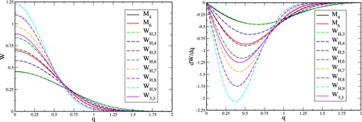
Comparison of the standard spline kernels M4 and M6 with the kernel family WH,n (kernels left, their derivatives right). Note that for ease of comparison the M6 kernel has been stretched to a support of Rk = 2. WH,3 is a close approximation of M4 and, if scaled to the same support, WH,5 is similar to M6. Also shown is the Wendland kernel W3,3.
Normalization constant σH,n of the WH,n kernels in one, two and three dimensions.
| Normalization σH,n of the WH,n kernels | |||||||
|---|---|---|---|---|---|---|---|
| n= 3 | n= 4 | n= 5 | n= 6 | n= 7 | n= 8 | n= 9 | |
| 1D | 0.660 203 38 | 0.752 215 01 | 0.834 353 71 | 0.909 204 80 | 0.978 402 21 | 1.043 052 35 | 1.103 944 01 |
| 2D | 0.450 733 24 | 0.580 312 18 | 0.710 379 46 | 0.840 709 99 | 0.971 197 17 | 1.101 784 66 | 1.232 440 06 |
| 3D | 0.317 878 09 | 0.458 917 52 | 0.617 012 65 | 0.790 449 59 | 0.977 949 35 | 1.178 510 74 | 1.391 322 15 |
4.1.2 Kernels with non-vanishing central derivatives
Here, we briefly discuss two kernel functions with non-vanishing central derivatives. The first example is the ‘linear quartic’ (LIQ) kernel that has been suggested (Valcke et al. 2010) to achieve a regular particle distribution and to improve SPH's performance in Kelvin–Helmholtz (KH) tests. The second example is shown mainly for pedagogical reasons: it illustrates how a very subtle change to the core of the well-appreciated M6 kernel seriously compromises its accuracy.
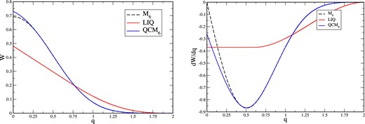
The peaked kernels LIQ and QCM6: kernel W on the left and its derivative dW/dq on the right. The QCM6 kernel has been constructed so that it hardly deviates from M6, but has a non-vanishing central derivative. For comparison also the M6 kernel plotted (dashed lines).
Parameters of the QCM6.
| Parameter | Numerical value |
|---|---|
| A | 11.017 537 |
| B | −38.111 922 |
| C | −16.619 585 |
| D | 69.785 768 |
| σ1D | 8.245 880 E-3 |
| σ2D | 4.649 647 E-3 |
| σ3D | 2.650 839 E-3 |
| Parameter | Numerical value |
|---|---|
| A | 11.017 537 |
| B | −38.111 922 |
| C | −16.619 585 |
| D | 69.785 768 |
| σ1D | 8.245 880 E-3 |
| σ2D | 4.649 647 E-3 |
| σ3D | 2.650 839 E-3 |
4.2 Accuracy assessment
4.2.1 Kernel support size
We give in Table 3 the values η that are used in the numerical experiments. They are chosen to be very large, but small enough to avoid pairing. Also given is the value qc, where |dW/dq| has its maximum, ηc = 1/qc and the corresponding neighbour number for a hexagonal lattice, Nc.
Values qc where the kernel derivative |dW(q)/dq| has the maximum, ηc = 1/qc. Nc is the neighbour number for a hexagonal lattice that corresponds to qc and η is the value used in our experiments. The latter has been chosen so that it is as large as possible without becoming pairing unstable, or, in cases where no pairing occurs, as large as computational sources allowed.
| Kernel | qc | ηc | Nc | η |
|---|---|---|---|---|
| M4 | 0.667 | 1.500 | 28 | 1.2 |
| M6 | 0.506 | 1.976 | 49 | 1.6 |
| WH,3 | 0.661 | 1.512 | 28 | 1.2 |
| WH,4 | 0.567 | 1.765 | 39 | 1.5 |
| WH,5 | 0.504 | 1.984 | 49 | 1.6 |
| WH,6 | 0.458 | 2.183 | 59 | 1.7 |
| WH,7 | 0.423 | 2.364 | 70 | 1.8 |
| WH,8 | 0.395 | 2.531 | 80 | 1.9 |
| WH,9 | 0.372 | 2.690 | 90 | 2.2 |
| W3,3 | 0.430 | 2.323 | n.a. | 2.2 |
| LIQ | n.a. | n.a. | n.a. | 2.2 |
| QCM6 | 0.506 | 1.976 | 49 | 2.2 |
4.2.2 Density estimates
To assess the density estimation accuracy, we perform a simple experiment: we place the SPH particles on a hexagonal lattice and assign all of them a constant value for the baryon number2, ν0. Since the effective area belonging to each particle with radius rs in a CP configuration is |$A_{\rm eff}= 2 \sqrt{3} r_{\rm s}^2$|, the theoretical density value is N0 = ν0/Aeff. We now measure the average relative deviation between the estimated and the theoretical density value, |$\epsilon _{N}= \sum _{a=1}^{N_{\rm part}} |N_a - N_0|/(N_0 \; N_{\rm part})$|, the results are shown in the left-hand panel of Fig. 4 as a function of the smoothing length parameter η, see equation (26). For clarity, we only show the odd members of the WH,n family. Note that we show the results up to large values of η where, in a dynamical simulation, some of the kernels would already have become pairing unstable. The ‘dips’ in the left-hand panel occur where the density error changes sign. The right-hand panel of Fig. 4 illustrates this for the case of the M4 kernel.
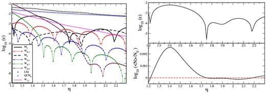
Accuracy of density estimates for different kernels. Particles are placed on a hexagonal lattice so that the density is uniform and the SPH density estimate is compared with the theoretical value to calculate the relative density error, see the left-hand panel. The parameter η determines the smoothing length, |$h_a= \eta V_a^{1/D}$|; LIQ: linear-quartic, QCM6: quartic core M6. To clarify the nature of the ‘dips’ in the left-hand panel, we plot in the right-hand panel the logarithm of the relative density error (upper right) and log (〈N〉/N0) for the case of the cubic spline kernel M4. The dips occur when the density error changes sign (exact value is indicated by the dashed red line).
The ‘standard’, cubic spline kernel M4 does not perform particularly well and simply replacing it by, say, the M6 kernel increases the density estimate already by roughly two orders of magnitude. If larger smoothing length can be afforded, however, the density estimate can be further substantially improved. For example, the WH,9 kernel for η > 2 achieves in this test approximately four orders of magnitude lower errors than what the M4 can achieve for η = 1.2 (for larger values it becomes pairing unstable). The Wendland kernel achieves a continuous improvement in the density estimate with increasing η and, as Dehnen & Aly (2012) argue, this protects the kernel against becoming pairing unstable. Although the W3,3 results in this test are less accurate than those of the higher order WH,n kernels, we gave preference to the Wendland kernel as our standard choice, since W3,3 allows only for very little noise, see below.
Both peaked kernels perform very poorly in this test, even for a very large support. It is particularly interesting to observe how the subtle change of the core of the M6 kernel (compare dashed black and the blue curve in Fig. 3) seriously compromises the density estimation ability (compare the dashed black curve with the blue triangles in Fig. 4).
4.2.3 Gradient estimates
We repeat the experiment described in Section 3.6 with the ‘standard’ SPH gradient, equation (6), for a number of different kernels. We set up particles on a 2D hexagonal lattice in [−1, 1] × [−1, 1], corresponding to a CP distribution of spheres with radius rs. All particles possess the same baryon numbers νb and are assigned pressures that rise linearly with the x-coordinate so that the slope is (∂xP) = 1. In Fig. 5, we show the impact of the kernel choice on the gradient accuracy (again, the M6 is stretched to a support of 2h). The M6 kernel (dashed black) yields, roughly speaking, a two orders of magnitude improvement over the standard SPH kernel M4 (solid black). Provided one is willing to apply larger neighbour numbers, the accuracy can be further improved by using smoother kernels. Once more, the high-order members of the WH,n kernel family perform very well for large η values. And, again, the Wendland kernel continuously improves the gradient estimate with increasing η. None of peaked kernels reaches an accuracy substantially below 10−2, not even for very large η-values.
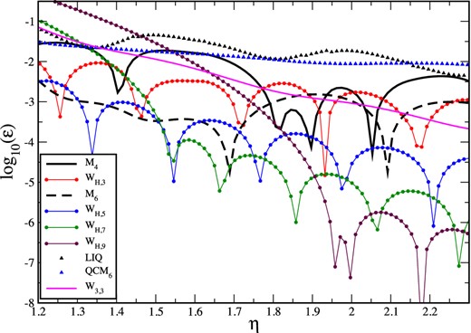
Accuracy of gradient estimates (calculated via equation 6) for different kernels. Particles are placed on a hexagonal lattice so that the density is uniform and the pressure linearly increasing. The parameter η determines the smoothing length, |$h_a= \eta V_a^{1/D}$|; LIQ: linear-quartic, QCM6: quartic core M6.
5 GENERALIZED VOLUME ELEMENTS
Here, we discuss the volume elements that are needed for the kernel techniques described in Section 3. In the following discussion, we use the baryon number ν and the CF baryon number density N, but every relation straight forwardly translates into Newtonian SPH by simply replacing ν with the particle mass m and N with the mass density ρ.
At contact discontinuities, the pressure is continuous, but density and internal energy suffer a discontinuity. For a polytropic equation of state (EOS), P = (Γ − 1)un, where n is the baryon number density in the local rest frame,3 the product of density and internal energy must be the same on both sides of the discontinuity to ensure a single value of P at the discontinuity, i.e. n1u1 = n2u2. Here, the subscripts label the two sides of the discontinuity. If this constraint is violated on a numerical level, say, because density and internal energy have a different smoothness across the discontinuity, spurious forces occur that act like a surface tension. This can occur in ‘standard’ SPH formulations since the density is estimated by a kernel-weighted sum over neighbouring particles and therefore is smooth, while the internal energy is a property assigned to each particle that enters ‘as is’ (i.e. un-smoothed) in the SPH evolution equations. Such spurious surface tension forces can compromise the ability to accurately handle subtle fluid instabilities, see for example Agertz et al. (2007), Springel (2010a) and Read et al. (2010). One may, however, question whether an unresolvably sharp transition in u is a viable initial condition in the first place. Note that Godunov-type SPH formulations (Inutsuka 2002; Cha & Whitworth 2003; Cha, Inutsuka & Nayakshin 2010; Murante et al. 2011; Puri & Ramachandran 2014) do not seem to suffer from such surface tension problems.
The problem can be alleviated if also the internal energy is smoothed, for example by applying some artificial thermal conductivity. This approach has been shown to work well in the case of KH instabilities (Price 2008; Valdarnini 2012). But it is actually a non-trivial problem to design appropriate triggers that supply conductivity in the right amounts exclusively where needed, but not elsewhere. Artificial conductivity applied where it is undesired can have catastrophic consequences, say by spuriously removing pressure gradients that are needed to maintain a hydrostatic equilibrium.
An alternative and probably more robust cure comes from using different volume elements in the SPH discretization process. Saitoh & Makino (2013) pointed out that SPH formulations that do not include density explicitly in the equations of motion avoid the pressure becoming multivalued at contact discontinuities. Since the density usually enters the equation of motion via the choice of the volume element νa/Na (or ma/ρa, respectively, in the Newtonian case), a different choice can possibly avoid the problem altogether. This observation is consistent with the findings of Heß & Springel (2010) who used a Voronoi tessellation to calculate particle volumes. In their approach, no spurious surface tension effects have been observed. Closer to the original SPH spirit is the class of kernel-based particle volume estimates that have recently been suggested by Hopkins (2013) as a generalization of the Saitoh & Makino (2013) approach. In the following, we will make use of these ideas for our relativistic SPH formulations.
To illustrate the impact that the choice of the volume element has on the resulting pressure across a contact discontinuity, we perform the following experiment. We place particles on a uniform hexagonal lattice, assign baryon numbers so that the densities for x < 0 have value N1 = 1 and N2 = 2 for x > 0 and internal energies as to reproduce a constant pressure P0 = 1 on both sides, ui = P0/((Γ − 1)ni). Here, i labels the side and Γ = 5/3 is the polytropic exponent. Once set up, we measure the densities according to equation (36) and since here n = N, we calculate the pressure distribution across the discontinuity, once for each choice of X. The standard SPH volume element corresponding to weight factor X = ν produces a smooth density transition, see upper panel of Fig. 6 that together with the sharp change in u causes the ‘pressure blip’ (orange oval) that is also frequently seen in SPH shock tests and that is the reason behind the spurious surface tension forces discussed above. The same experiment, if repeated using X = Pk, does not show any noticeable deviation from the desired value of unity. The phenomenon of spurious surface tension is further explored by numerical experiments in Section 7.3.
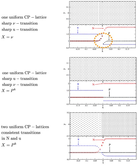
Different ways to set up a contact discontinuity. In the upper panel, particles are placed on a uniform hexagonal lattice (‘close packed’, CP) and masses/baryon numbers and internal energies are assigned as to reproduce the constant states, with a sharp transition at x = 0. Since the subsequent density calculation (with X = ν) produces a smooth density transition, the mismatch between a sharp internal energy u and a smooth density N leads to a ‘pressure blip’ (orange oval) that leads to spurious surface tension forces at the interface. If for the same setup X = Pk is used, both N and u have a sharp transition and the pressure blip disappears, see middle panel. The lower panel shows an alternative setup with equal masses/baryon numbers where the density structure is encoded in the particle distribution (here two uniform hexagonal lattices). The corresponding density calculation (with X = Pk) also produces a smooth density transition, but the internal energy is consistently (and therefore smoothly) assigned from the calculated density and the condition of uniform pressure.
As an alternative numerical model for a contact discontinuity, we show in the last panel of Fig. 6 a setup for the case of constant particle masses/baryon numbers. In this case, the information about the density is encoded in the particle distribution, for which we use here two uniform hexagonal lattices. Also here (X = Pk) the density transition is smooth, but the internal energy is calculated (via an iteration) from the condition of constant pressure, so that the smoothness of N and u are consistent with each other.
6 SPECIAL-RELATIVISTIC SPH
We will now apply the techniques discussed in Sections 3–5 to the case of ideal, special-relativistic fluid dynamics. Excellent descriptions of various aspects of the topic (mostly geared towards Eulerian methods) can be found in a number of recent textbooks (Alcubierre 2008; Baumgarte & Shapiro 2010; Goedbloed, Keppens & Poedts 2010; Rezzolla & Zanotti 2013). In a first step, see Section 6.1, we generalize the derivation from the Lagrangian of an ideal relativistic fluid to the case of the generalized volume elements as introduced in equation (38). This leads to a generalization of the kernel-gradient-based equations given in Rosswog (2010). In a second formulation, see Section 6.2, we use integral-based gradient estimates, see equation (25), again for the case of a general volume element.
6.1 Special-relativistic SPH with kernel derivatives
We assume a flat space–time metric, ημν, with signature (−,+,+,+) and use units in which the speed of light is equal to unity, c = 1. We reserve Greek letters for space–time indices from 0…3 with 0 being the temporal component, i and j refer to spatial components and SPH particles are labelled by a, b and k.
6.1.1 The general momentum equation
6.1.2 The general energy equation
6.1.3 Consistent values for smoothing lengths, densities and weights
The smoothing lengths, the CF density and possibly the weight X depend on each other. If the weight depends on the density, say for the case X = Pk, we first perform a few steps to find accurate values of the new pressure: (a) calculate new volumes according to equation (38) using the smoothing lengths and weights from the previous time step, (b) from the resulting new value of the density we update the pressure according to equation (62), (c) update the smoothing length according to equation (26) (d) once more update the volume and (e) again the pressure. This pressure value is finally used to perform an iteration between volume, equation (38), and the smoothing length, equation (26). Due to the previous steps, the guess values at this stage are already very accurate, so that on average only one iteration is needed to meet our convergence criterion |N(n+1) − N(n)|/N(n+1) < 10−4.
While this procedure requires a number of iterations, we find that it is worth the effort, since a careless update of the smoothing length can produce a fair amount of noise that can compromise the quality of a simulation. An inaccurate update of the smoothing lengths may be a largely overlooked source of noise in many SPH codes.
6.2 Special-relativistic SPH based on IAs to derivatives
In this scheme, the smoothing lengths are updated exactly as described above for the kernel-gradient based method, see Section 6.1.3.
6.3 Dissipative terms
6.3.1 Controlling the amount of dissipation: triggers on shocks and velocity noise
Artificial dissipation is really only needed under specific circumstances such as to produce entropy in shocks where it mimics nature's behaviour, though on a larger, resolvable scale. Nevertheless, in older SPH implementations artificial dissipation was (and still often is) applied everywhere, regardless of whether it is actually needed or not and, as a consequence, one is modelling some kind of a viscous fluid rather than the intended inviscid Euler equations.
Recently, Cullen & Dehnen (2010) suggested further improvements to the Morris & Monaghan (1997) approach. They argued that a floor value for the viscosity parameter is unnecessary and that the original scheme may, in some situations, be too slow to reach the required values of the dissipation parameter. They suggest to immediately raise the viscosity parameter to the desired value rather than obtaining it by integrating the above ODE. Moreover, and as already noted in the original paper of Morris & Monaghan (1997), a scheme with the originally suggested source term, equation (81), would also spuriously trigger on a constant slow compression with |$\nabla \cdot \boldsymbol {v}$|= const. Therefore, Cullen & Dehnen (2010) suggested to trigger on the time derivative of |$\nabla \cdot \boldsymbol {v}$|. They further pointed out that |$\nabla \cdot \boldsymbol {v}$| as calculated by standard SPH gradients can have substantial errors which trigger unnecessary dissipation in shear flows even if standard shear-limiters (Balsara 1995) are used.
The noise trigger of equation (88) actually only triggers on the signs of |$\nabla \cdot \boldsymbol {v}$| and does not take into account how substantial the compressions/expansions are compared to the ‘natural scale’ cs/h. The above noise trigger therefore switches on even if the fluctuation is not very substantial, but only causes a very small level of the dissipation parameter (∼0.02 for our typical parameters, see below). One might therefore, alternatively, consider to simply apply a constant ‘dissipation floor’ Kmin. We chose, however, the trigger-version, both for the aesthetic reason that we do not want untriggered dissipation and since the triggered version shows a slightly higher convergence rate in the Gresho–Chan test. The differences, however, are not very significant.
The functioning of our dissipation triggers is illustrated in Fig. 32.
6.4 Recovery of the primitive variables
Similar to many grid-based approaches, we have to pay a price for the simplicity of the evolution equations (55)/(61) or (64)/(65) with the need to recover the physical variables from the numerical ones (Chow & Monaghan 1997; Rosswog 2010). The strategy is to express all variables in equation (62) in terms of the updated variables |$\boldsymbol {S}, \epsilon , N$| and the pressure P, then solve for the new pressure, and finally substitute backwards until all physical variables are available.
6.5 Time integration
7 MULTIDIMENSIONAL BENCHMARK TESTS
All of the following tests, whether in the Newtonian or special-relativistic regime, are performed with a new 2D SPH code, called sphincs_sr. At the current stage, it is by no means optimized, its entire purpose is to explore different (special-relativistic) SPH formulations.
In the following, we scrutinize the effects of the different new elements in number of benchmark tests by using four different SPH formulations:
Formulation 1 (|$\mathcal {F}_1$|):
Density: equations (36) and (38) with weight X = Pk, k = 0.05
Momentum equation: equation (64)
Energy equation: equation (65)
Kernel: Wendland kernel W3,3 with η = 2.2, see equation (26)
We expect results of similar quality for the WH,9 kernel, but since the Wendland kernel W3,3 produced less noise in the ‘noise box’ and the Gresho–Chan vortex test we chose it as our default kernel.
Formulation 2 (|$\mathcal {F}_2$|):
Density: equations (36) and (38) with weight X = Pk, k = 0.05
Momentum equation: equation (55)
Energy equation: equation (61)
Kernel: Wendland kernel W3,3 with η = 2.2, see equation (26)
The difference between |$\mathcal {F}_1$| and |$\mathcal {F}_2$| measures the impact of the different gradient prescriptions.
Formulation 3 (|$\mathcal {F}_3$|):
Momentum equation: equation (64)
Energy equation: equation (65)
Kernel: Wendland kernel W3,3 with η = 2.2, see equation (26)
Same as |$\mathcal {F}_1$|, but with the more ‘standard’ choice X = ν to explore the impact of volume element.
Formulation 4 (|$\mathcal {F}_4$|):
Momentum equation: equation (55)
Energy equation: equation (61)
Dissipative terms: see Section 6.3, use equation (76), constant dissipation parameter K = 1
Kernel: M4 kernel with η = 1.2, see equation (26)
These are choices close to what is used in many SPH codes. As will become clear below, these are rather poor choices, i.e. in many cases the accuracy of a code could be substantially increased by a number of relatively simple measures with respect to ‘standard recipes’.
Usually, we will focus on the results of the |$\mathcal {F}_1$| formulation, but when larger deviations for other formulations occur, we also show a brief comparison.
All of the following tests are performed with the special-relativistic code sphincs_sr. But since the discussed improvements are not specific to special relativity but instead concern SPH techniques in general, we discuss both Newtonian and special-relativistic tests. Each of the tests is marked accordingly: ‘N’ for Newtonian and ‘SR’ for special relativity.
7.1 Initial particle distribution (N/SR)
The initial conditions and in particular the initial particle distribution are crucial for the accuracy of an SPH simulation. Of course, the quality indicators |$\mathcal {Q}_{1}$|–|$\mathcal {Q}_{4}$|, equations (4) to (9), should be fulfilled to good accuracy and this suggests to use some type of lattice. Unfortunately, this is not enough and the particle distribution should have at least two more properties: (a) it should be stable for the used SPH formulation–lattice combination, i.e. particles in pressure equilibrium should remain in their configuration and (b) there should not be preferred directions in the particle distribution. Condition (a) means that the particles should be in a minimum energy configuration and how this relates to the kernel choice and the form of the SPH equations is from a theoretical point of view poorly understood to date. Simply placing particles on some type of lattice is usually not good enough: the particles will in most cases begin moving off the lattice and introduce noise. We will explore this explicitly in Section 7.2. Condition (b) is necessary since preferred directions can lead to artefacts, for example, a shock travelling along a preferred direction of a lattice will collect preferentially particles in this direction and this can lead to unwanted ‘ringing’ effects. An example of this effect is shown in Fig. 17.
In the following tests, we will, as a default, place the SPH particles on a hexagonal lattice, see Fig. 7, upper-left panel, but if artefacts can occur we will use a ‘glass-like’ particle distribution instead (upper-rightmost panel). To produce the glass, our strategy is to start from a hexagonal lattice, perturb it heavily and subsequently drive that particles into positions so that they represent a good partition of unity, see equation (4). We proceed according to the following steps.
Place the desired number of particles on a hexagonal lattice (upper-left panel) corresponding to the closest packing of spheres with radii rs, where each particle has an effective volume of |$2 \sqrt{3} r_{\rm s}^2$| (Fig. 7, first panel, upper row).
Apart from ‘frozen’ boundary particles, perturb the particles heavily by displacing them by a distance r0 = 0.9rs in a random direction (Fig. 7, second panel, upper row).
- The perturbed particle distribution is then driven to a good partition of unity by applying pseudo-forces proportional to the negative gradient of the quality indicator |$\mathcal {Q}_1$|, see equation (4). Since in the end we want a uniform particle distribution so that all volumes Vb should finally be the same, V0, we take the volumes out of the sum, use a uniform smoothing length |$h_0= 2.2 \sqrt{V_0}$| and as pseudo-force simplytogether with the Wendland kernel. The maximum value of all particles at the initial, heavily perturbed distribution is denoted |$\boldsymbol {f}_{\rm max}^0$|. Obviously, equation (101) just corresponds to a force opposite to the gradient of the SPH particle number density as measured via a kernel summation, so driving the particles to a uniform number density.(101)\begin{equation} \boldsymbol {f}_a= - \sum _b \nabla _a W_{ab}(h_a) \end{equation}
- As a next step, an iteration is performed. Rather than really using an acceleration and a time step, we apply a displacement so that the particle with the maximum force |$\boldsymbol {f}_{\rm max}^0$| is allowed to be displaced in the first iteration by a distance r0 = 0.5rs and in all subsequent iterations byThis iteration is performed until max|$_a (|\delta \boldsymbol {r}_a|)/r_{\rm s} < 10^{-3}$|. Since the algorithm is designed to take small steps, it takes a large number of steps to meet the convergence criterion (several hundreds for the above parameters); however, the iterations are computationally inexpensive, since they can all be performed with a once (generously large) created neighbour list, so that neighbours only need to be searched once.(102)\begin{equation} \delta \boldsymbol {r}_a = \frac{r_0}{f_{\rm max}^0} \boldsymbol {f}_a. \end{equation}
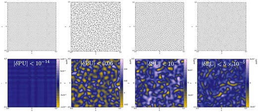
Particle distributions (first row): initial hexagonal lattice (left-hand column), heavily perturbed hexagonal lattice (second column), after 10 iterations (third column) and final distribution (fourth column). The second row shows the deviation from a partition of unity, δPU. Note that the colour bar shows vastly different scales.
7.2 Static I: ‘Noise box’ (N)
To date, there is still only poor theoretical understanding which particle configurations represent stable minimum energy configurations and how this depends on the chosen kernel. As a heuristic approach, one can apply a ‘relaxation method’ where artificial damping is used to drive the particles into a near-optimal configuration. However, this can be very time consuming, it is not necessarily clear when the equilibrium has been reached and the approach can become very challenging in practice for complicated initial conditions.
Often, the particles are simply placed on a lattice which ensures accurate interpolation properties, see Sections 3.1 and 3.2, but this does not guarantee that the particles are in a stable equilibrium position. In practice, for most kernel–lattice combinations the particles will start ‘moving off the lattice’ and keep moving unless they are explicitly damped. It has been observed (Springel 2010a) that this moving-off-the-lattice can hamper proper convergence in KH instabilities and, as we will see below, it also plays a major role in the convergence of the Gresho–Chan vortex problem.
We perform here a simple experiment where we place 10K particles in the domain [0,1] × [0,1] so that their density is N = 1 and their pressure is P = 100 everywhere (Γ = 5/3). We add margins of three smoothing lengths with of ‘frozen boundary particles’ at each side. We perform the experiment twice, once with a hexagonal or ‘CP’ (‘CP-lattice’; left-hand panel in Fig. 8) and once with a quadratic lattice (‘Q-lattice’; right-hand panel in Fig. 8). Ideally, these configurations should be perfectly preserved. Subsequently, we let the inner particles evolve freely (in practice we set our noise parameter to |$\mathcal {N}_{\rm \; \; noise}= 10^6$|, see equation 94, so that the noise trigger does not switch on and no dissipation is applied) and thereby monitor the average particle velocity (in units of the sound speed, 〈v〉/cs) as a function of time (in units of the sound crossing time, τs).
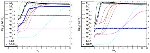
Results of the ‘noise box test’ for an initial hexagonal (left) and Q-lattice (right). Shown is the logarithm of the average particle velocity (in units of the sound speed) as a function of time (in units of the sound crossing time through the computational domain). For both initial lattice configurations and nearly all kernel choices, the particles start eventually moving off the lattice and move with average velocities of 1–2 per cent of the speed of sound. For the hexagonal lattice, only the cubic spline kernel (solid black, right-hand panel; ‘M4’) and the Wendland kernel (W3,3) are stable. For the Q-lattice only, the modified quintic spline kernel (blue triangles; ‘QCM6’) retains the particles in their original configuration on the time-scale of the experiment.
There are a number of interesting conclusions from this experiment. First, for almost all kernel choices, the particles eventually move off the initial lattice and move with average velocities of 1–2 per cent of the sound speed. Interesting exceptions are the cubic spline kernel for which the hexagonal lattice seems to be a stable minimum energy configuration (〈v〉/cs ≈ 10−4). The Wendland kernel W3,3 remains to an even higher accuracy (〈v〉/cs ≈ 5 × 10⁻⁷) on the CP lattice. The WH,9-kernel remains for around three sound crossing times perfectly on the CP lattice, but then the particles begin to move and settle to a noise level comparable to the lower order kernels (〈v〉/cs ≈ 10−2). It is also interesting that kernels that are naively expected to be close approximations to each other show a very different behaviour in this test. The WH,3-kernel, which closely approximates M4, see Fig. 2, shows a very different noise behaviour: at the chosen η (=1.2, like M4), it already starts forming pairs while M4 stays nearly perfectly on the CP lattice. Also, the WH,5-kernel is substantially more noisy than the original M6-kernel. The modified quintic spline kernel, QCM6, although not very accurate in previous tests, see Figs 4 and 5, shows actually only little noise. It does not stay on the CP lattice, but nevertheless only produces little noise (〈v〉/cs ≈ 5 × 10⁻³), and it is the only kernel that remains exactly on the Q-lattice (〈v〉/cs < 10−6). Both the WH,9- and the W3,3-kernels move off the Q-lattice after about three sound crossing times, but W3,3 shows a much lower noise level (〈v〉/cs < 10−3 versus ≈10−2).
The behaviour in this ‘noisebox test’ is consistent with the results in the Gresho–Chan vortex, see Section 7.4, where noise is one of the accuracy-limiting factors. Also in this latter test, the W3,3 shows the least noise, followed by the QCM6-kernel, which performs even better than WH,9. Interestingly, there seems to be no clear relation between the degree of noise and the kernel order, at least not for the explored initial configurations. The stability properties of particle distributions deserve more theoretical work in the future.
7.3 Static II: surface tension test (N)
As discussed in Section 5, depending on the initial setup, the standard choice for the SPH volume element Vb = νb/Nb (or Vb = mb/ρb in the Newtonian case) can lead to spurious surface tension forces across contact discontinuities which can prevent subtle instabilities from growing.
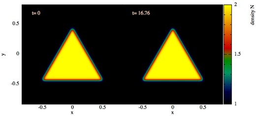
To test for the presence of such a spurious surface tension for the different choices of the volume element, we set up the following experiment. We distribute 20K particles homogeneously on a hexagonal lattice within an outer box of [−1, 1] × [−1, 1]. For the triangular central region with edge points (|$-0.5,-\sqrt{3}/4$|), (|$0.5,-\sqrt{3}/4$|) and (|$0,\sqrt{3}/4$|), we assign the density Ni = 1.0, the outer region has density No = 2.0, the pressure is P = P0 = 2.5 everywhere and the polytropic exponent is chosen as Γ = 5/3. Ideally, the system should stay in exactly this state if it is allowed to evolve. Possibly, present spurious surface tension forces would have the tendency to deform the inner triangle into a circle. We perform this test with formulation |$\mathcal {F}_1$| and |$\mathcal {F}_3$|, but the only difference that matters here is the volume element. In fact, after only t = 5 or about 2.6 sound crossing times, the standard X = ν-discretization has already suffered a substantial deformation, see Fig. 9, while |$\mathcal {F}_1$| does not show any sign of surface tension and is indistinguishable from the original configuration (left-hand panel). The choice X = 1, by the way, yields identical results to X = Pk.
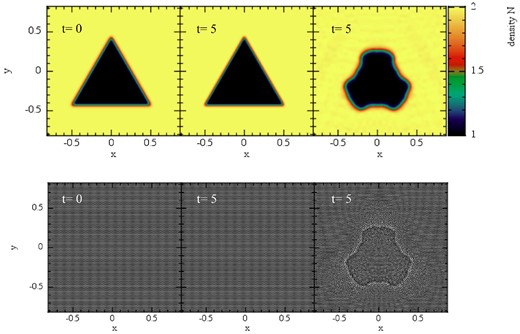
Surface tension test: evolution of a triangular region in pressure equilibrium with its surroundings. The first row shows the density N, the second the corresponding particle distribution. The first column shows the initial condition, the second column the result for weighting factor X = Pk (visually identical to the results obtained with X = 1) and the last column shows the result for the standard SPH volume choice (X = ν corresponding to Vb = νb/Nb, or, Vb = mb/ρb in Newtonian language). The standard SPH volume choice shows at t = 5 already strong deformations that are the result of spurious surface tension forces. The alternative choices X = Pk and X = 1 (not shown) perfectly preserve the original shape.
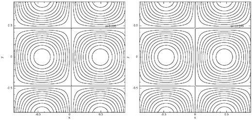
7.4 Gresho–Chan-like vortex (N)
The differential rotation displaces the particles from their original hexagonal lattice positions and therefore introduces some amount of noise. The noise trigger |$\mathcal {N}_{\rm \; \;1}$|, see equation (88), triggers local values of Ka of up to 0.04, |$\mathcal {N}_{\rm \; \;2}$| does not switch on, just as it should. Also, the shock trigger works very well and does practically not switch on at all: in an initial transient phase, it suggests (still negligible) values for the dissipation parameter Ka of ∼10−3 and then decays quickly to <10−6. We have used this test to gauge our noise triggers. We find good results for a noise reference value of |$\mathcal {N}_{\rm \; \; noise} = 50$|, this will be explored further below.
As a first test, we compare the performance of the different formulations |$\mathcal {F}_1$| to |$\mathcal {F}_4$| for 50K particles, see Fig. 10 .
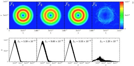
Performance of the different SPH formulations in the Gresho–Chan vortex test (from left to right column: |$\mathcal {F}_1$| to |$\mathcal {F}_4$|; snapshots are shown at t = 1, all 50K particles are displayed). The upper row shows |$|\boldsymbol {v}|$| colour-coded in the x–y-plane, the lower row shows the velocity as a function of the distance to the vortex centre. In the lower row also the L1-error is indicated. The constant high dissipation in |$\mathcal {F}_4$| seriously deteriorates the result compared to |$\mathcal {F}_1$| to |$\mathcal {F}_4$|. The impact of the integral-based versus kernel-derivative gradients can be judged by comparing |$\mathcal {F}_1$| (integral-based; first column) to |$\mathcal {F}_2$| (kernel gradient based; otherwise identical; second column). The choice of the volume element hardly makes a difference in this test (see |$\mathcal {F}_1$| versus |$\mathcal {F}_3$|).
To better understand the role of the chosen kernel function, we perform an additional experiment, where we use the best SPH formulation, |$\mathcal {F}_1$|, but vary the kernel (with the smoothing lengths as indicated in Table 3). As already noticed in the ‘noise-box’ test, different kernels exhibit different levels of noise which is crucial for the accuracy in this test. In Fig. 11, we show the results for 25K particles for the CS, M6, WH,9 and the W3,3 kernel. The upper row shows the velocity, colour-coded as function of the position, the lower row displays the velocity as function of the distance to the vortex centre. For our chosen noise reference value |$\mathcal {N}_{\rm \; \; noise}$|, only very little dissipation is released in response to particle noise. Therefore, at the shown time t = 1, the triangular velocity shape is still reasonably well captured in all cases, though with substantial noise overlaid in all cases but WH,9 and W3,3. A large fraction of the error is due to the particles moving off their original hexagonal lattice. These results are consistent with the findings from the ‘noise box’ test, see above, and show once more that the W3,3 kernel only produces a very small amount of noise in comparison to the other explored kernels. We have run this test for the peaked kernels, each time with the same support as the W3,3 kernel (η = 2.2), not shown. While the LIQ kernel performs poorly and produces very noisy results with a large error (L1 = 6.06 × 10⁻²), the QCM6 kernel performs again astonishingly well, though not as good as W3,3. It produces symmetric, relatively noise-free results with an error of only L1 = 1.06 × 10⁻², actually even slightly better than the WH,9 kernel (L1 = 1.58 × 10⁻²).
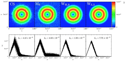
Performance of different kernels in the Gresho–Chan vortex test. All tests used 25K particles and the SPH formulation |$\mathcal {F}_1$| (apart from the kernel choice, of course), results are shown at t = 1. Upper row: |$|\boldsymbol {v}|$| in x–y-plane, lower row: |$|\boldsymbol {v}|$| as a function of the distance from the vortex centre. From left to right: cubic spline, quintic spline, WH,9 and Wendland kernel. In the lower row also the L1 error norm of the velocity is given. Clearly, the Wendland kernel produces the most accurate result.
We also explore the convergence with the effective, one-dimensional particle number N1D of the different formulations in Fig. 12. Clearly, the ‘standard SPH recipe’ formulation |$\mathcal {F}_4$| (blue triangles) performs very poorly, consistent with the findings of Springel (2010a) who concludes that (standard) SPH does not converge to the correct solution. Both our formulations |$\mathcal {F}_1$| (black circles) and |$\mathcal {F}_3$| (green diamonds) converge roughly linearly (long-dashed line). The kernel-gradient version |$\mathcal {F}_2$| converges roughly |$\propto \!N_{\rm 1D}^{-0.6}$|, consistent with the findings of Dehnen & Aly (2012). Recently, also Hu et al. (2014) have implemented a number of worthwhile modifications into the gadget code (Springel 2005) that substantially improve the convergence in the Gresho–Chan vortex. They measured a convergence rate close to 0.8. Read & Hayfield (2012) report a convergence rate close to 0.9.
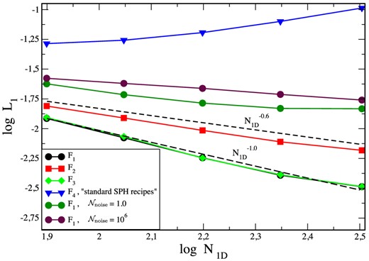
Convergence in Gresho–Chan vortex test. Our best SPH formulation |$\mathcal {F}_1$| converges close to linearly with the effective, one-dimensional particle number N1D (long-dashed line), |$\mathcal {F}_3$| performs very similar. Our version with kernel derivatives, |$\mathcal {F}_2$|, converges somewhat slower, roughly |$\propto\! N_{\rm 1D}^{0.6}$| (short-dashed line), consistent with the findings of Dehnen and Aly (2012). The noise trigger clearly improves the convergence, both too little (|$\mathcal {N}_{\rm \; \; noise}= 10^6$|) and too high sensitivity (|$\mathcal {N}_{\rm \; \; noise}= 1.0$|) to noise deteriorate the convergence rate. The ‘standard SPH recipe’ formulation, |$\mathcal {F}_4$|, fails this test rather catastrophically.
We also perform experiments to explore the impact of the noise trigger on the convergence: once we run the test without dissipation (in practice |$\mathcal {N}_{\rm \; \; noise}= 10^6$|) and once we deliberately apply too much dissipation (|$\mathcal {N}_{\rm \; \; noise}= 1.0$|). In the first case, there is steady (though slower, approximately |$\propto\! N_{\rm 1D}^{-0.6}$|) convergence, whereas the excessive dissipation in the second case seems to hamper convergence. The moderately triggered dissipation by noise therefore increases the convergence rate. This is our main motivation for using the noise trigger |$\mathcal {N}^{(1)}$|, see equation (88). For many tests, however, we would expect to obtain very similar results even if this (small) source of dissipation was ignored.
7.5 Advection tests (SR)
For our Lagrangian schemes, advection tests do not represent any particular challenge since the code actually has not much to do apart from accurately recovering the primitive variables and advancing the particle positions. Therefore, advection is essentially perfect. We briefly demonstrate the excellent advection properties in the two following tests.
7.5.1 Advection I
In this first test, we start from the configuration of the surface tension test, see Section 7.3, with 7K particles placed inside the domain [−1, 1] × [−1, 1]. We now give each fluid element a velocity in x-direction of vx = 0.9999 corresponding to a Lorentz factor of γ ≈ 70.7 and apply periodic boundary conditions. In Fig. 13, we show the results for the |$\mathcal {F}_1$| equation set. After 10 times crossing the computational domain,5 the shape of the triangle has not changed in any noticeable way. The |$\mathcal {F}_2$| results are visually identical, |$\mathcal {F}_3$| and |$\mathcal {F}_4$| (not shown) deform the triangle like in the previous surface tension test.
Advection test 1: the initial density pattern shown on the left, constant pressure everywhere, is advected with vx = 0.9999 (c = 1) corresponding to a Lorentz factor γ = 70.7 through the computational domain with periodic boundary conditions. Right-hand panel: shape after 10 times crossing the computational domain.
7.5.2 Advection II
Advection test 2: a density pattern is advected with a velocity of 0.9 c (γ = 2.29) through a box with periodic boundaries. The initial condition (t = 0.000) is shown in the left-hand panel, the result after crossing the box five times (t = 10.299) is shown on the right.
7.6 Riemann problems (SR)
Since we have tested a large variety shock benchmark tests in previous work (Rosswog 2010, 2011) and the results of the new formulations do not differ substantially in shocks, we restrict ourselves here to a few standard shock tests and focus on multidimensional tests where either the differences due to the new numerical elements are more pronounced or where SPH has been criticized to not perform well.
7.6.1 Riemann problem I: Sod-type shock
This mildly relativistic shock tube (γmax ≈ 1.4) has become a widespread benchmark for relativistic hydrodynamics codes (Marti & Müller 1996; Chow & Monaghan 1997; Siegler 2000; Del Zanna & Bucciantini 2002; Marti & Müller 2003). It uses a polytropic exponent of Γ = 5/3, vanishing initial velocities everywhere, the left state has a pressure PL = 40/3 and a density NL = 10, while the right state is prepared with PR = 10−6 and NR = 1.
We place 50K particles initially on a hexagonal lattice in [−0.4, 0.4] × [−0.02, 0.02], with particles in the low-density region being rotated by 30°, see below, and use our standard parameter set. The SPH result of the |$\mathcal {F}_1$| formulation (squares, at t= 0.3) agrees very well with the exact solution (solid line), see Fig. 15. Only directly after the shock front some ‘re-meshing noise’ is visible. This is unavoidable since the particles have to move from their initial configuration into a new one which also involves small velocity components in y-direction. This re-meshing noise could be further reduced by applying more dissipation, though at the price of reducing the height of the density plateau near x = 0.25. Note, that with the presented dissipation scheme the theoretical density peak is reached with only 50K particles while in earlier work (Rosswog 2010) it was hardly reached even with 140K particles. This is mainly due to the new shock trigger where the dissipation parameter peaks ∼2 smoothing lengths ahead of the shock and starts decaying immediately after, similar to the case of the Cullen & Dehnen (2010) shock trigger.
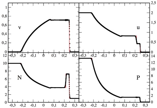
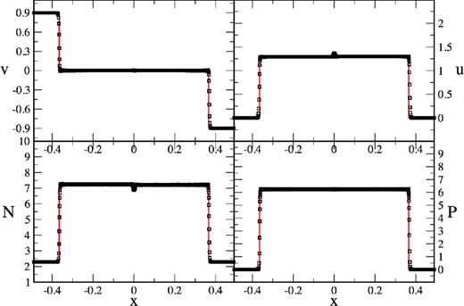
2D relativistic Sod-type shock tube at t = 0.3. The SPH result (|$\mathcal {F}_1$| formulation, 50K particles; note that every particle is shown, i.e. no averaging has been applied) is shown as black squares, the red line is the exact solution.
A comparison between the different formulations for only 20K particles (at t = 0.3) is shown Fig. 16. We focus on the post-shock plateau of N since here dissipation effects are particularly visible. The |$\mathcal {F}_1$| formulation delivers the cleanest and ‘edgiest’ result. Note that the choice of X = ν (|$\mathcal {F}_3$|) introduces additional density oscillations. This ‘lattice-ringing’ phenomenon at low dissipation using the standard volume element (i.e. for |$\mathcal {F}_3$|) has been observed in a number of the following tests (KH instabilities, Section 7.7.1), the blast–bubble interactions and the ‘blast-in-a-box’ problem, see Section 7.8). The clearly worst, excessively dissipative result is obtained with formulation |$\mathcal {F}_4$|.
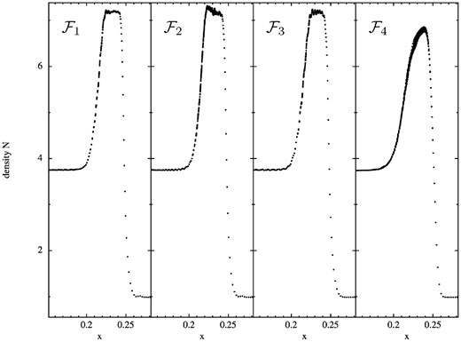
Low-resolution (20K particles) 2D Sod shock tube test. Shown is the post-shock density plateau at t = 0.3 for the SPH formulations |$\mathcal {F}_1$| to |$\mathcal {F}_4$| (left to right). The plateau is best captured by the formulations that use the integral-based kernel (|$\mathcal {F}_1$| and |$\mathcal {F}_3$|), among them the version with volume weight X = Pk (|$\mathcal {F}_1$|) shows fewer oscillations. The version with weight X = Pk but direct kernel gradients (|$\mathcal {F}_2$|) still works reasonably well, but the ‘standard SPH recipe’ formulation (|$\mathcal {F}_4$|) is excessively dissipative. Note that the small oscillations in the plateau could be further reduced, though at the expense of more dissipation.
In the previous cases, we had rotated the particle distribution on the RHS by 30° to avoid continuously collecting particles along the direction of motion. We illustrate the impact of this measure in the experiment shown in Fig. 17, left-hand panel: we set up a low-resolution (5K particles) version of the above test, once we use the same lattice orientation on both sides (left-hand column, left-hand panel) and once we rotate the distribution by 30° (right-hand column, left-hand panel). While both cases capture the overall solution well, the case without rotation shows a substantial ‘re-meshing noise’ behind the shock while in the rotated case the particles remain well ordered without much velocity noise. Such noise could be removed by adding more dissipation, but rotating the particle distribution is certainly the better option. In the right-hand panel of Fig. 17, we show the results of another experiment (30K particles) where we demonstrate the working of our dissipation triggers. The dissipation parameter K is shown together with the desired values from the noise trigger. We also show the values for the entropy function A, as reconstructed from pressure and density via A = P/nΓ.
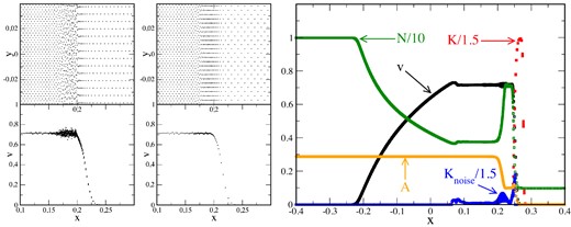
Left: the importance of the initial particle lattice is illustrated by zooming into the shock front of a low-resolution, 2D, relativistic Sod simulation (5K particles). The left-hand column shows the result (particle distribution, above, and velocity, below) for the case where on both sides of the shock a hexagonal lattice with a symmetry axis along the shock motion direction was used. The only difference in the right-hand column is that the initial lattice on the right-hand side was rotated by 30°. This substantially reduces the ‘re-meshing noise’ in the velocity (near x ≈ 0.2) behind the shock. Right: 2D shock tube test (30K particles) where also the dissipation parameter K is shown (red). The blue circles show the parameter values suggested by the noise trigger, the orange symbols show the values of the entropy function A = P/nΓ.
7.6.2 Riemann problem II: relativistic Planar Shock Reflection
As a second problem, we show the result of another standard relativistic shock benchmark test where two gas streams collide, see e.g. Hawley et al. (1984), Eulderink & Mellema (1995), Falle & Komissarov (1996) and Aloy et al. (1999). We use a polytropic exponent of Γ = 5/3 and the left and right state are given by [n, vx, vy, u]L = [1.0, 0.9, 0.0, 2.29 × 10⁻⁵] and [n, vx, vy, u]R = [1.0, −0.9, 0.0, 2.29 × 10⁻⁵], where the incoming velocities correspond to Lorentz factors of γ = 2.29. The result from a simulation with 160K particles initially placed on a hexagonal lattice between [−2.0, 2.0] × [−0.05, 0.05] at t = 0.875 is shown in Fig. 18. Overall, there is excellent agreement with the exact solution (red line), only at the centre an ‘overheating’ or ‘wall heating’ phenomenon occurs in the density and internal energy. This is a well-known phenomenon (Norman & Winkler 1986; Noh 1987; Eulderink & Mellema 1995; Mignone & Bodo 2005) that plagues a large number (if not all) shock-capturing schemes (including, e.g. the Roe, HLLE and HLLC Riemann solvers).
2D, relativistic planar shock reflection test where two gas streams collide with vx = ±0.9c. The exact solution is shown by the solid, red line the SPH solution (|$\mathcal {F}_1$| formulation, t = 0.875) is shown as black squares.
As a more extreme version of this test, we use initial velocities of 0.9995c, i.e. [n, vx, vy, u]L = [1.0, 0.9995, 0.0, 2.29 × 10⁻⁵] and [n, vx, vy, u]R = [1.0, −0.9995, 0.0, 2.29 × 10⁻⁵]. Here, the incoming velocities correspond to Lorentz factors of γ = 31.6. We use the same setup as above, but only 80K particles in the same computational domain. Also in this extreme test, the solution is robustly and accurately captured, see Fig. 19. The solution with the |$\mathcal {F}_1$| formulation and our standard parameter set is shown (at t = 0.5) as blue circles and agrees very well with the exact solution (red line). Only at the origin, a wall-heating phenomenon occurs in the internal energy and the density. As an experiment, we repeat the same test with exactly the same setup and parameters, but now we use a dissipation floor Kmin = 1, see equation (82). The continued dissipation reduces the amount of wall heating. This is consistent with earlier studies, e.g. Noh (1987) and Rosswog & Price (2007), that find that wall heating is reduced by applying artificial conductivity. The other formulations perform similar well, with differences consistent with those seen in Riemann problem I (see Fig. 16): |$\mathcal {F}_2$| and |$\mathcal {F}_3$| show slightly larger oscillations in the shocked region, |$\mathcal {F}_4$| leads to rounder edges, but also, like the black square solution in Fig. 19, to a slightly quieter shocked region and reduced wall heating due to the larger dissipation.
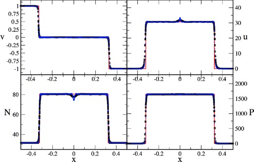
Two-dimensional, relativistic planar shock reflection test where two gas streams collide with vx = ±0.9995c. The exact solution is shown by the solid, red line the SPH solution (|$\mathcal {F}_1$| formulation, t = 0.5) is shown as blue circles for our standard parameter set and as black squares for the same parameters but a dissipation floor Kmin = 1, see equation (82).
7.6.3 Riemann problem III: Einfeldt-type rarefaction test
Here, we explore the ability to properly capture rarefaction waves by means of an Einfeldt-type (Einfeldt et al. 1991) test. The initial conditions6 are given by [n, vx, vy, P]L = [0.1, −0.5, 0.0, 0.05] and [n, vx, vy, P]R = [0.1, 0.5, 0.0, 0.05], so that two rarefaction waves (γ ≈ 1.15) are launched in opposite directions. This test had originally been designed to point out a failure mode of Riemann solvers that can return negative densities or pressures in strong rarefaction waves. We setup this test with only 5K particles, placed on a hexagonal lattice between [−0.45, 0.45] × [−0.05, 0.05]. Note that despite the very low particle number, the results of the numerical simulation (|$\mathcal {F}_1$|-formulation; squares; t = 0.3) agree very well with the exact solution (red, solid line), see Fig. 20.
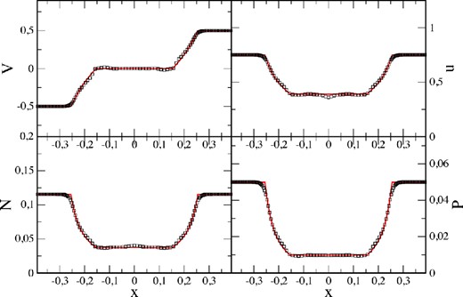
Result of a 2D, Einfeldt-type rarefaction test. The SPH solution (at t = 0.3) is shown as black squares, the exact result as solid, red line. Note that only 5000 particles have been used for this two-dimensional test.
7.7 Fluid instabilities (N)
7.7.1 KH instabilities
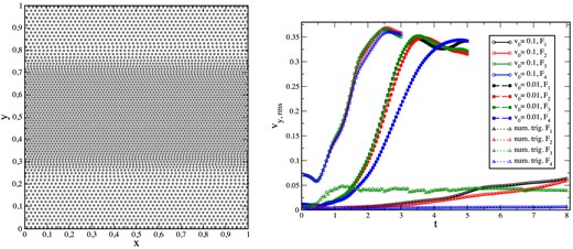
Left-hand panel: example of a ‘quasi-CP’ particle distribution (8K particles) for a KH experiment that produces for equal-mass particles a double-step density distribution. Right-hand panel: growth of the rms y-velocity component as a function of time in the different experiments. The solid lines with circles refer to the strongly triggered cases (vy, 0 = 0.1; up to t = 3), dashed lines with squares to the weakly triggered experiments (vy, 0 = 0.01; up to t = 5) and dotted lines with triangles to the numerically triggered experiments (up to t = 8).
The results for vy,0 = 0.1 for the different formulations |$\mathcal {F}_1$| (top row) to |$\mathcal {F}_4$| (bottom row) are shown in Fig. 22, each time at t = 0.5, 1.0, 2.0 and 3.0. Overall, there is good agreement between the different SPH formulations, all show a healthy KH growth. Only |$\mathcal {F}_4$| is, as expected, excessively diffusive. In the vy,0 = 0.01 case, the instability grows slower; therefore, we show in Fig. 23 snapshots at t = 1.0, 3.0, 4.0 and 5.0. Once more, all formulations, even the worst and most diffusive |$\mathcal {F}_4$|, are able to capture the instability. This is different from the findings of Garcia-Senz et al. (2012), their standard SPH formulation does not show a healthy growth, despite their slightly larger particle number (62.5K compared to our 50K). The difference may come from subtleties, for example, they use particles of different masses while we use equal-mass particles. Their particles are placed on a Q-lattice (which is not an equilibrium configuration, see Section 7.2) while ours are on a hexagonal lattice. Moreover, since we apply the dissipation to the numerical variables, see Section 6.3, which contain also the specific energy, this introduces a small amount of conductivity, which might help the instability to grow (Price 2008). Last but not least, we have found that the exact algorithm for the smoothing length update can introduce a fair amount of noise. In our algorithm, we have taken particular care to avoid noise and to have consistent values to a very high accuracy, see Section 6.1.3.
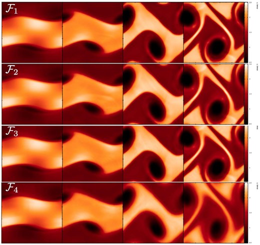
Comparison of the performance of the different formulation (with 50K particles; colour-coded is the density N) in a KH test triggered by a moderate initial velocity perturbation of vy,0 = 0.1. Each row corresponds to the result of one formulation (top to down: |$\mathcal {F}_1$| to |$\mathcal {F}_4$|), each of the panels in one row refers to t= 0.5, 1.0, 2.0 and 3.0. The |$\mathcal {F}_1$| formulation performs best, but the differences between the different formulations are overall only moderate.
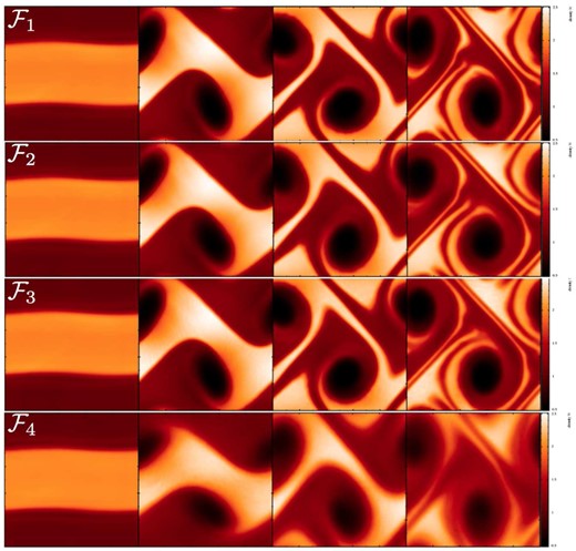
Comparison of the performance of the different formulation (with 50K particles; colour-coded is the density N) in a KH test triggered by a small initial velocity perturbation amplitude of only vy,0 = 0.01. Each row corresponds to the result of one formulation (top to down: |$\mathcal {F}_1$| to |$\mathcal {F}_4$|), each of the panels in one row refers to t = 1.0, 3.0, 4.0 and 5.0. All cases show a healthy growth of the instability despite the only very small perturbation.
In a further KH test, no particular mode is excited and the instability is seeded numerically. To this end, we place 200K particles in three stripes of cubic lattices in the computational domain [−1, 1] × [−1, 1], with high-density strip of N = 2 moving with v = 0.2 to the right, while the low-density strips with N = 1 move with v = −0.2 to the left, the pressure is P = 10 and the polytropic exponent Γ = 5/3. The results are shown in Fig. 24 at times t = 4.0, 6.0 and 8.0. In all cases apart from |$\mathcal {F}_4$|, a KH instability with the characteristic billows develops. In the very diffusive |$\mathcal {F}_4$| case, perturbations still grow at the end of the simulation, but at an extremely slow pace. Note that in the case of the ‘standard’ SPH volume element, |$\mathcal {F}_3$|, small vibrations in the particle distributions emerge which appear in the plot as an overlaid ‘grid-like’ pattern (this is not an artefact of the visualization). Such vibrations have also been observed in other tests with |$\mathcal {F}_3$|, see for example Fig. 16. Comparing |$\mathcal {F}_1$| and |$\mathcal {F}_2$| one sees that the more accurate integral-based gradients resolve sharper features in comparison to the kernel-based variant.
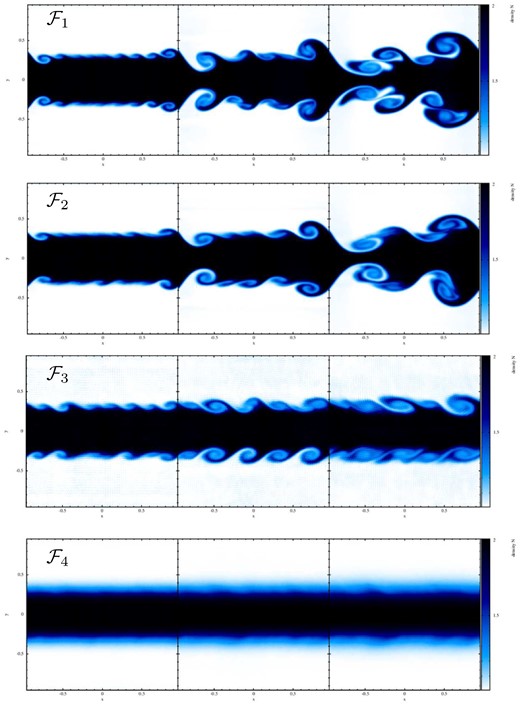
Numerically triggered KH instability (200K particles; colour-coded is the density N). The high-density band (N = 2) initially moves at −0.2c to the left, while the low-density bands (N = 1) move at 0.2c to the right. No particular mode is excited, the instability grows from small numerical perturbations as the particles at the interface pass along each other. Snapshots are shown at t = 4.0, 6.0 and 8.0 (left to right) for the SPH formulations |$\mathcal {F}_1$| (top) to |$\mathcal {F}_4$|(bottom). Note that the grid-like structure for the |$\mathcal {F}_3$| result is not an artefact of the visualization, here the particles vibrate around their lattice positions.
As a last example, we follow the evolution of 1000K particles with the |$\mathcal {F}_1$| formulation, again without explicitly triggering a particular mode, we simply wait until small numerical perturbations grow into healthy KH billows, see Fig. 25.
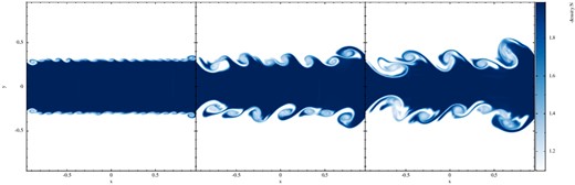
Growth of a KH instability (|$\mathcal {F}_1$|-formulation) that has not been triggered explicitly (1000K particles). The density N is shown at t = 2.0, 4.0 and 5.25.
7.7.2 Rayleigh–Taylor instabilities
The Rayleigh–Taylor (RT) instability is another classical test case. In its simplest form, it occurs when a denser fluid rests on top of a lighter one in a gravitational field. When perturbed, the denser fluid begins to sink down and the release of gravitational energy triggers a characteristic, ‘mushroom-like’ flow pattern, both for the lighter fluid rising up and the heavier one sinking down. Generally, SPH is thought to be seriously challenged in dealing with RT instabilities, but as we will show below, the suggested measures provide a major improvement also in this case.
The hydrodynamic evolution for |$\mathcal {F}_1$| to |$\mathcal {F}_4$| is shown (each time at t = 2.5, 5.0 and 8.25) in Fig. 26. Consistent with the findings of other tests, |$\mathcal {F}_1$| develops the finest density structures and the instability grows fastest. The results for |$\mathcal {F}_2$| and |$\mathcal {F}_3$| are not very different, though, they also show a healthy growth of RT mushrooms. Like in the untriggered KH case, the ‘standard method approach’ |$\mathcal {F}_4$| fails completely and does not allow the weakly triggered instability to grow.
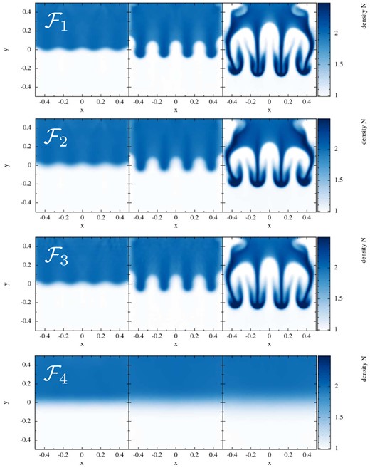
Growth of a weakly triggered RT instability (50K particles) for the SPH formulations |$\mathcal {F}_1$| to |$\mathcal {F}_4$|. For each formulation, the snapshots are taken at t = 2.5, 5.0 and 8.25.
In modern adaptive mesh refinement simulations, e.g. Keppens et al. (2012), secondary KH events occur on the falling spikes/pillars. The resolution in our tests is not large enough to resolve them. This is mainly due to the large smoothing length required for the Wendland kernel and due to the use of equal-mass/baryon number particles which lead to particularly low resolution in the low-density regions.
7.8 Combined tests
We also perform a number of more complex tests for which no exact solutions are available and the results need to be compared to other methods documented in the literature. These tests illustrate the robustness and flexibility of the new approaches and demonstrate that a complex interplay between shocks, rarefaction and fluid instabilities can be handled with ease.
7.8.1 Relativistic blast–bubble interaction I (SR)
In Fig. 27, we show the density at t = 90, 180, 270, 360, 450, as in the original paper, for the |$\mathcal {F}_1$| formulation. The results agree excellently with those found in the relativistic adaptive mesh refinement approach of He & Tang (2012), see their figs 13 and 14, including the shape and location of the various travelling waves.
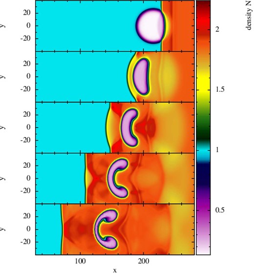
Blast–bubble interaction I: a blast wave is impacting from the right on to a low-density bubble in pressure equilibrium. This test has been performed with the |$\mathcal {F}_1$| formulation and 100K particles. Snapshots are shown at t = 90, 180, 270, 360 and 450.
To explore the impact of the various new ingredients, we repeated this test for formulations |$\mathcal {F}_1$| to |$\mathcal {F}_4$| with only 50K particles. A comparison of the results at t = 500 is displayed in Fig. 28. |$\mathcal {F}_1$| clearly performs best, |$\mathcal {F}_4$| does not capture any of the ‘curling in’ of the upper and lower lobe. Here, the gradient accuracy seems crucial (compare |$\mathcal {F}_1$| and |$\mathcal {F}_3$| with |$\mathcal {F}_2$| and |$\mathcal {F}_4$|).
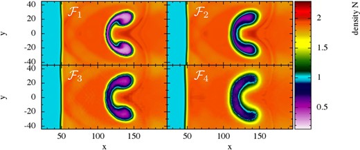
Comparison of different approaches for blast–bubble interaction I for low resolution (50K particles; at t = 500). Once more, the |$\mathcal {F}_1$| formulation clearly performs best, both gradient accuracy (compare |$\mathcal {F}_1$| and |$\mathcal {F}_2$|) and the volume element (upper row versus lower row) impact on the result.
7.8.2 Relativistic blast–bubble interaction II (SR)
This test is similar to the previous one, but now the bubble has a larger density of N = 3.1538, as in He & Tang (2012), their example 6.9. The higher density results in a different flow pattern, just as in non-relativistic hydrodynamics. This setup results in mildly relativistic velocities (v ≈ 0.35, γ ≈ 1.07). Fig. 29 shows snapshots (200K particles) at t = 100, 200, 300, 400 and 500, just as in the original paper. Again, we find excellent agreement with their results. We again explore the sensitivity to our new ingredients by re-running this test with formulations |$\mathcal {F}_1$| to |$\mathcal {F}_4$| with only 50K particles. The results at t = 500 are displayed in Fig. 30. The tendencies are similar to the previous test. While |$\mathcal {F}_1$| to |$\mathcal {F}_3$| show reasonable agreement, |$\mathcal {F}_1$| shows the cleanest, oscillation-free bubble surface. |$\mathcal {F}_1$| and |$\mathcal {F}_3$| at least show a vague reminiscence of the ‘hole’ near x = 160, y = 0 that is found in high-resolution case. For such small-scale features, the gradient accuracy seems crucial. Again, some oscillations appear for |$\mathcal {F}_3$| near x = 180). Not much structure is visible in the case of |$\mathcal {F}_4$| due to the very large dissipation and surface tension effects.
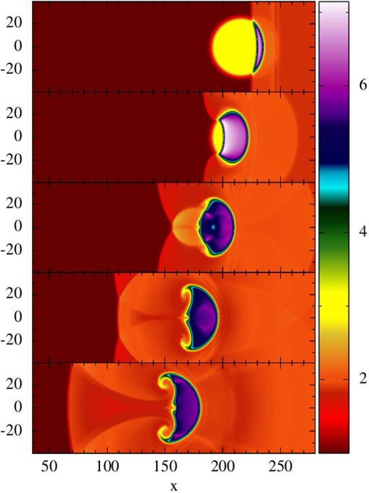
Blast–bubble interaction II: a blast wave is impacting from the right on to a high-density bubble in pressure equilibrium. This test has been performed with the |$\mathcal {F}_1$| formulation and 200K particles. Snapshots are shown at t = 100, 200, 300, 400 and 500. Colour-coded is the CF baryon density N.
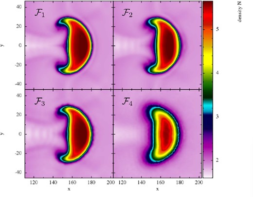
Comparison of different approaches |$\mathcal {F}_1$| to |$\mathcal {F}_4$| for a low-resolution comparison of blast–bubble interaction II test (50K particles; t = 500).
7.8.3 ‘Blast in a box’ (SR)
This test simulates an overpressured central region that expands in a perfectly, spherically symmetric manner. Once the blast is reflected by the boundaries, a complicated interaction between shock–shock and shock–contact discontinuities sets in. In the Newtonian setup of, e.g. Stone et al. (2008), these interactions create the Richtmyer–Meshkov instabilities in the central low-density region. The Richtmyer–Meshkov instabilities in this test are a serious challenge for SPH simulations since they occur in the lowest density regions which are very poorly resolved. Therefore, we run this test at a relatively large resolution (600K particles), but also compare low-resolution simulations (200K) of the different formulations.
In this test, we have experimented somewhat with the initial particle setup, since lattices may lead to a ‘pile up’ of particles in certain directions. We have experimented with a particle setup as described in Section 7.1, but since the combination of Wendland kernel and IA-gradient produces also very symmetrical results for a hexagonal lattice we use for simplicity such a setup in the following tests.
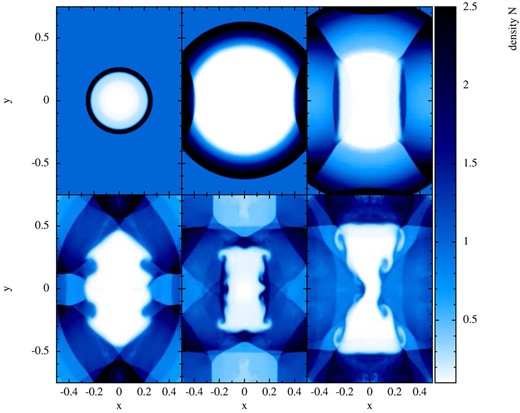
Blast in a box: shown are snapshots at t = 0.2, 0.7, 1.0, 2.0, 3.0, 4.0 (left to right, top to bottom, |$\mathcal {F}_1$|) of the CF baryon number density. Note the mushroom-like structures appearing in the central and upper/lower parts of panels 5 and 6.
To illustrate the working of the dissipation switches in such a geometrically complicated situation, we show in Fig. 32 snapshots at t = 0.5 of the simulation shown in Fig. 31. As can be seen from the lower left panel, the shock trigger really only switches on at the shock location, where it produces a razor-sharp circle of high K-values. The noise trigger produces dissipation where particles are arranging themselves after the shock as passed.
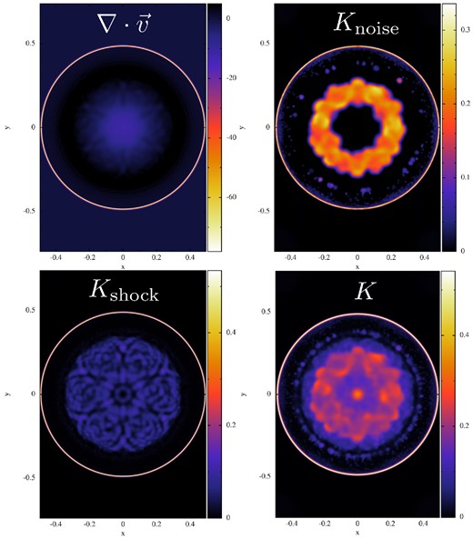
Illustration of the dissipation switches at the ‘blast in a box’ problem (at t = 0.5). Shown are snapshots of |$\nabla \cdot \boldsymbol {v}$|, upper left, the instantaneous value of Knoise, added to calm down particles when they are noisy, see equation (93), upper right, the instantaneous value of Kshock, see equation (86), lower left, and the currently used value of K.
We also briefly compare the four SPH formulations for the case where only 200K particles are used, see Fig. 33. in the low-density central region. Vague anticipations of the Richtmyer–Meshkov instabilities appear in |$\mathcal {F}_1$| to |$\mathcal {F}_3$|, but not in |$\mathcal {F}_4$|. The Richtmyer–Meshkov instabilities for |$\mathcal {F}_2$| seem actually slightly more pronounced than those of |$\mathcal {F}_1$|. We attribute this to the larger noise level for the case of kernel-gradient formulations that helps triggering the instabilities. The mushroom-like structure near x = 0 at the upper and lower boundaries are most developed for |$\mathcal {F}_1$|. As outlined above, however, the major deficiency here is simply the lack of resolution.
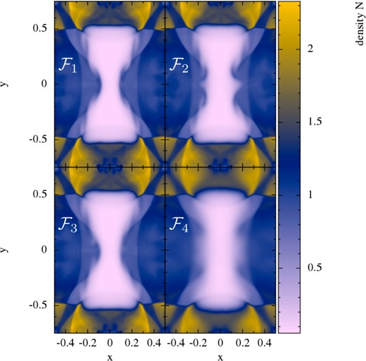
Comparison of the different formulations (|$\mathcal {F}_1$|, upper left, to |$\mathcal {F}_4$|, lower right) for a low-resolution version (200K) of the ‘blast-in-box’ test.
We use this to compare the new gradient prescription with the standard, kernel-gradient approach. We use 200K particles and compare |$\mathcal {F}_1$| and |$\mathcal {F}_2$|. In Fig. 34, we show density snapshots at t= 0.3. At this stage, the pattern should be perfectly spherically symmetric; however, in the |$\mathcal {F}_2$| case the sixfold symmetry of the underlying hexagonal lattice becomes visible while |$\mathcal {F}_1$| shows practically perfect symmetry. Note, however, that a special colour scheme was chosen to make the noticeable but still moderate differences visible.
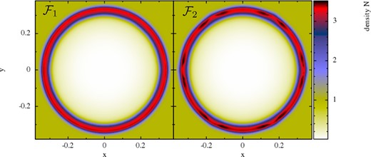
Comparison between the IA-gradient (|$\mathcal {F}_1$|, left) and the standard kernel gradient (|$\mathcal {F}_2$|, right) for a low-resolution version (200K) of the ‘blast-in-box’ test. The IA-gradient shows essentially perfect symmetry while the kernel-gradient shows signs of sixfold symmetry of the underlying hexagonal particle lattice. Note, however, that the differences are small and a particular colour scheme has been chosen to them well visible.
We perform another test to compare the performance of different kernels under challenging conditions. In particular, we are interested in the level of noise and the question whether the grid symmetries are reflected in aggregated quantities such as the density. To this end, we performed this test with the |$\mathcal {F}_1$| formulation, but once we use the CS kernel (η = 1.2), once the M6 kernel (η = 1.6), once WH,9 (η = 2.2) and once the Wendland kernel W3,3 (η = 2.2). For this test, 79K particles were used. The results at t = 0.45, just before the shock hits the first set of walls, is shown in Fig. 35. The first row shows the density N and the second and third one show |$\nabla \cdot \boldsymbol {v}$| which is a sensitive indicator for the presence of noise. The kernel functions are noted in the panels. Clearly, after the passage of the shock the particles have to re-arrange themselves into a new configuration, so some particle motion and therefore a non-zero value of |$\nabla \cdot \boldsymbol {v}$| is expected. The cubic spline kernel produces the noisiest results, followed by M6 and the higher order kernels. The Wendland kernel performs slightly better than WH,9, especially close to the explosion centre where it produces the most symmetric results of all kernels. It is also the only kernel that does not show any sign of the sixfold symmetry of the original hexagonal lattice configuration. Consistent with our previous tests, the Wendland kernel produces the cleanest and least noisy results.
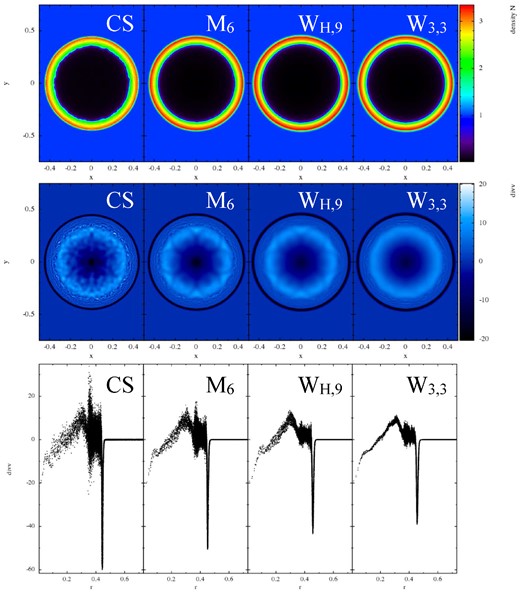
Importance of the kernel choice in the ‘blast-in-a-box’ test. All tests are performed with the |$\mathcal {F}_1$| formulation, apart from the kernel choice. The upper row shows the CF baryon number density and the other rows show |$\nabla \cdot \boldsymbol {v}$| as an indicator for the presence of noise, one colour-coded in the XY-plane (middle) and once as function of the distance from the explosion centre (bottom). The first column shows the result for the cubic spline kernel (η = 1.2), the second the M6 kernel (η = 1.6) and column three and four show the results for WH,9 and the Wendland kernel (both with η = 2.2).
8 SUMMARY
In this paper, we have explored the impact of various SPH discretization choices. Motivated by future relativistic applications, we have developed a 2D special-relativistic SPH code, called sphincs_sr, that allows us to explore a large number of different choices. All the tests of this paper – whether in the Newtonian or special-relativistic limit – have been performed with this new code. Part of the motivation of this paper was to show that modern SPH formulations perform very well even in challenging tests where more traditional SPH approaches fail badly.
The effects of the improvements are the following.
Gradients
The first measure concerns the calculations of gradients. We have explored here in particular a prescription that starts from an integral-based function representation and requires the (analytical) inversion of a small matrix. By neglecting appropriate terms, one can recover the same desirable antisymmetry property in particle indices as the standard SPH kernel gradient (for radial kernel functions). Thus, numerical conservation can be ensured in a similar manner as in standard SPH. Such gradient prescriptions had been explored earlier in an astrophysical context by Garcia-Senz et al. (2012) and Cabezon et al. (2012) and, in an engineering context, by Jiang et al. (2014). As we show in Section 3.6, the gradient accuracy can be dramatically increased (∼ 10 orders of magnitude!) if the particle distribution is regular, see Fig. 1. The new prescription also yields much more accurate results under less idealized circumstances. The SPH formulations with the new gradient prescriptions are able to resolve smaller details and they result in less velocity noise (compare |$\mathcal {F}_1$| and |$\mathcal {F}_3$|), see, for example, Figs 10 and 16. Moreover, the gradient prescription turns out to be very beneficial in resolving fluid instabilities, see Section 7.7.
Kernel choice
Apart from the commonly used, ‘standard’ SPH kernel M4 and the M6 kernel, we have explored examples of peaked kernels and in particular some high-order members of a recently suggested kernel family (Cabezon et al. 2008) and a high-order Wendland kernel (Wendland 1995). We found that the most commonly used SPH kernel M4 actually performs rather poorly, see for example Figs 4, 5, 11 and 35. The M6 kernel is better, but the results still can be substantially improved by employing higher order kernels. The overall best performance was found for the Wendland kernel. It allows for only very little velocity noise, even in highly dynamical situations, see Figs 8, 11 and 35. The explored peaked kernels performed very poorly in practically every respect, even for very large kernel supports.
Volume elements
Motivated by recent suggestions of Saitoh & Makino (2013) and Hopkins (2013), we have generalized our previous relativistic SPH formulation to a class of more general volume elements, see equation (38), that differ from the traditional choice m/ρ in the Newtonian and ν/N in the special-relativistic case. We have in particular explored the case where the weighting quantity is a power of the pressure, |$X_b= P_b^k$|, k = 0.05. This formulation removes spurious surface tension effects, see Fig. 9, and it performs in all of the tests at least as good, but sometimes substantially better than the standard choice Xb = νb (corresponding to the usual SPH density sum). In fact, for the standard SPH choice Xb = νb together with low dissipation, we have seen in a number of tests ‘lattice ringing effects’, see for example, Figs 24, 30, 28 and 33. Other choices for the weight X are certainly possible and should be explored in future studies.
Dissipation triggers
We have also designed new triggers to decide where dissipation should be applied. Our general strategy is ‘react immediately, decay fast’: if the triggers indicate a desired value that is higher than the currently used value, the dissipation parameter is raised immediately to the indicated value (Cullen & Dehnen 2010) and subsequently it decays exponentially on a very short time-scale. We trigger on both shocks and velocity noise. Our shock trigger is based on the temporal change of the velocity divergence, very similar to the approach of Cullen & Dehnen (2010). We also trigger on the occurrence of velocity noise, see equations (88) and (92). The first of these noise triggers only releases very little dissipation, based on fluctuations in the sign of |$\nabla \cdot \boldsymbol {v}$|. This small amount of extra dissipation substantially improves the convergence rate in the Gresho–Chan test, see Fig. 12, but for a number of tests probably very good results would be obtained even if this trigger was ignored. The second trigger hardly ever switches on, but when it does so, it efficiently damps possibly remaining post-shock oscillations/noise. The addition of such noise triggers allows us to safely choose a very short decay time for the dissipation parameter, since possibly appearing noise is efficiently taken care of. An illustration of the functioning of our dissipation triggers is shown in Figs 17 and 32. In summary, our treatment takes at each time step for each particle a decision on the required dissipation value. This leads to a very local dissipation and essentially removes unwanted effects while providing accurate and robust solutions, even in strong shocks, see Section 7.6.
To disentangle the different effects in benchmark tests, we use four different SPH formulations, in the paper referred to as |$\mathcal {F}_1$| to |$\mathcal {F}_4$|, which are explained in detail at the beginning of Section 7. The first one, |$\mathcal {F}_1$|, contains all suggested improvements, while |$\mathcal {F}_4$| uses every time the worst choices (CS-kernel, direct kernel derivatives, standard SPH volume element and constant, large dissipation parameters), choices that are actually not too far from what is implemented in a number of frequently used SPH codes. The |$\mathcal {F}_1$| formulation delivers excellent results, even in those tests where the ‘standard choices’ fail completely. For example, |$\mathcal {F}_4$| does not converge to the correct solution in the Gresho–Chan vortex, consistent with earlier findings of Springel (2010a), while |$\mathcal {F}_1$| converges in this test close to linearly. Another example are the weakly triggered or untriggered fluid instabilities, see Sections 7.7.1 and 7.7.2, where |$\mathcal {F}_4$| hardly shows any evolution at all while all other formulations show a healthy growth of the instabilities.
We have found |$\mathcal {F}_1$| to be a major improvement over commonly made choices, whether in Newtonian or relativistic tests. So far, no efforts have been undertaken to optimize any of the SPH formulations in terms of computational speed and in this form |$\mathcal {F}_1$| takes approximately twice as much time as |$\mathcal {F}_4$|, mainly due to the required matrix inversion and the substantially larger neighbour number (η = 2.2 rather than 1.2; see equation 26). While we think that the results more than justify the additional computational effort even in the purely hydrodynamic case, the inclusion of other physics ingredients such as self-gravity may actually make the extra effort practically negligible.
In recent years, a number of projects have been carried out to compare numerical hydrodynamics methods that are commonly used in astrophysics (Price & Federrath 2010; Creasey et al. 2011; Bauer & Springel 2012; Scannapieco et al. 2012; Sijacki et al. 2012; Torrey et al. 2012; Bird et al. 2013; Hayward et al. 2014; Hubber, Falle & Goodwin 2013; Nelson et al. 2013). At least to some extent, these investigations were triggered by Lagrangian Voronoi-tesselation codes having become available both for Newtonian (Springel 2010b) and special-relativistic hydrodynamics (Duffell & MacFadyen 2011). Where shortcomings of SPH were identified, they were attributed to excessive dissipation, velocity noise and gradient accuracy. As demonstrated in this study, all these issues can be substantially improved by the suggested measures. Comparisons of the suggested |$\mathcal {F}_1$| SPH formulation (or its Newtonian equivalents) with other methods are left to future studies.
It is a pleasure to acknowledge inspiring discussions with Daniel Price and Joe Monaghan during a sabbatical stay at Monash University. Also the hospitality of the University of Queensland in Brisbane and Monash University, Clayton, Vic 3800, Australia is gratefully acknowledged. The stay in Australia was supported by the DFG by a grant to initiate and intensify bilateral collaboration. This work has further been supported by the Deutsche Forschungsgemeinschaft (DFG) under grant number RO-3399/5-1, by the Swedish Research Council (VR) under grant 621-2012-4870 and by the CompStar network, COST Action MP1304. This work has profited from visits to Oxford which were supported by a DAAD grant ‘Projektbezogener Personenaustausch mit Großbritannien’ under grant number 313-ARC-XXIII-Ik and from visits to La Scuola Internazionale Superiore di Studi Avanzati (SISSA), Trieste, Italy. It is a pleasure to acknowledge in particular the hospitality of John Miller (Oxford, Trieste). SR also gratefully acknowledges the hospitality of Andrew MacFadyen (New York University) and of Enrico Ramirez-Ruiz (UC Santa Cruz) and their home institutions where part of this work was carried out. The stay in Santa Cruz was generously supported by the David and Lucile Packard Foundation. Many of the figures of this article were produced with the visualization software splash (Price & Monaghan 2007). The author also thanks Marius Dan and Franco Vazza for their careful reading of the manuscript. It is a pleasure to acknowledge detailed conversations with Walter Dehnen and to thank him for his insightful comments and a number of useful suggestions.
We use the convention that W refers to the full normalized kernel while w is the un-normalized shape of the kernel.
This is equivalent to assigning a constant particle mass for the Newtonian case.
As will be described in more detail below, we measure energies here in units of the baryon rest mass energy m0c2. The Newtonian correspondence of the expression is, of course, P = (Γ − 1)uρ.
We express here everything in terms of our notation where the dissipation parameter is called K. In the literature on non-relativistic SPH, the dissipation parameters are usually called α and β. To translate our approach to non-relativistic SPH, one may replace K by α and choose β as a multiple (usually = 2) of α.
The numerical value, t = 16.76, comes from our periodic boundaries being four smoothing length inside the nominal box boundaries.
Note that we are specifying here local rest-frame densities rather than CF densities. This is simply for a straightforward comparison with the analytical result obtained by the code ‘riemann-vt.f’ from Marti & Müller (2003).
