


Abstract
We present an analysis of the diffuse emission at 5 GHz in the first quadrant of the Galactic plane using two months of preliminary intensity data taken with the C-Band All-Sky Survey (C-BASS) northern instrument at the Owens Valley Radio Observatory, California. Combining C-BASS maps with ancillary data to make temperature–temperature plots, we find synchrotron spectral indices of β = −2.65 ± 0.05 between 0.408 and 5 GHz and β = −2.72 ± 0.09 between 1.420 and 5 GHz for −10° < |b| < −4°, 20° < l < 40°. Through the subtraction of a radio recombination line free–free template, we determine the synchrotron spectral index in the Galactic plane (|b| < 4°) to be β = −2.56 ± 0.07 between 0.408 and 5 GHz, with a contribution of 53 ± 8 per cent from free–free emission at 5 GHz. These results are consistent with previous low-frequency measurements in the Galactic plane. By including C-BASS data in spectral fits, we demonstrate the presence of anomalous microwave emission (AME) associated with the H ii complexes W43, W44 and W47 near 30 GHz, at 4.4σ, 3.1σ and 2.5σ, respectively. The CORNISH (Co-Ordinated Radio ‘N’ Infrared Survey for High mass star formation) VLA 5-GHz source catalogue rules out the possibility that the excess emission detected around 30 GHz may be due to ultracompact H ii regions. Diffuse AME was also identified at a 4σ level within 30° < l < 40°, −2° < b < 2° between 5 and 22.8 GHz.
1 INTRODUCTION
Diffuse Galactic radio emission is a combination of free–free, synchrotron, anomalous microwave and thermal dust emission. Below 10 GHz, free–free and synchrotron contributions account for the majority of the emission, while anomalous microwave emission (AME) reaches its peak between 10 and 30 GHz (Gold et al. 2009; Planck Collaboration XV 2014). At frequencies >100 GHz, the total Galactic emission is dominated by thermal emission from dust (Finkbeiner & Schlegel 1999). Measurements of the diffuse Galactic emission are used for both the interpretation of cosmological data and the understanding of our Galaxy. Synchrotron emission can reveal information on the Galactic magnetic field and cosmic ray physics (Jaffe et al. 2011) while free–free emission measurements can be used to explore H ii regions and the warm ionized medium (WIM; Davies et al. 2006). The cosmological demand for increasingly sensitive, large-scale maps of Galactic emission is driven by the need to remove these ‘foreground’ emissions to obtain an accurate measurement of the cosmic microwave background (CMB) signal. This is particularly the case for imaging the CMB polarization signal and identifying B-modes, where the intrinsic cosmological signal is a small fraction of the foregrounds (Betoule et al. 2009; Dunkley et al. 2009; Errard & Stompor 2012; Bennett et al. 2013). This issue has been exemplified by the recent claim of a detection of intrinsic CMB B-modes (Ade et al. 2014), which now appears to be contaminated by foregrounds (Planck Collaboration XXX 2014).
As different foregrounds dominate over different spectral and spatial ranges, it is important to have all-sky data available covering a range of frequencies and with ∼1° resolution if CMB polarization experiments are to live up to their full potential in determining cosmological parameters (Planck Collaboration XII 2014). The low-frequency all-sky intensity surveys currently most used for this purpose are at 0.408 GHz (Haslam et al. 1982), 1.420 GHz (Reich & Reich 1986; Reich, Testori & Reich 2001; Testori et al. 2001), 22.8 GHz (Bennett et al. 2013) and 28.4 GHz (Planck Collaboration I 2014). Jonas, Baart & Nicolson (1998) and Carretti et al. (2013) provide Southern hemisphere maps at 2.3 GHz in intensity and polarization, respectively. Sun et al. (2007) present a polarization survey of the Galactic plane at 5 GHz with a full width at half-maximum (FWHM) of 9.5 arcmin so as to capture the small-scale structures. However, the lack of all-sky, degree scale surveys between 1.420 and 22.8 GHz introduces great uncertainties in the spectral behaviour of free–free, synchrotron and AME across the full sky (Peel et al. 2012).
C-BASS, the C-Band All-Sky Survey, is a project currently mapping Galactic intensity and linear polarization at a frequency of 5 GHz (Jones et al. in preparation, King et al. 2010). At this frequency, the polarized emission is negligibly affected by Faraday rotation at high latitudes (Δψ ≲ 1° across most of the |b| > 10° latitude sky). C-BASS consists of two independent telescopes: C-BASS North observes from the Owens Valley Radio Observatory (OVRO) in California, USA (latitude 37| $_{.}^{\circ}$|2 N) whilst C-BASS South is located at the Klerefontein support base for the Karoo Radio Astronomy Observatory (latitude 30| $_{.}^{\circ}$|7 S). C-BASS North achieved first light in 2010 and entered its final survey mode in late 2012 after a period of commissioning and upgrades (Muchovej et al. in preparation). C-BASS South is currently being commissioned. The final all-sky maps will have an FWHM resolution of 43.8 arcmin and a nominal sensitivity in polarization of ≈0.1 mK per beam. On completion, the C-BASS data will be used to probe the Galactic magnetic field using synchrotron radiation, constrain the spectral behaviour of AME, and provide a polarized foreground template for CMB polarization experiments. The large angular scale and high sensitivity of the final survey will be of particular use for confirming B-mode detections at low multipoles.
In this paper, we present some of the Galactic science that can be achieved using preliminary C-BASS intensity results. We focus on the composition of the Galactic plane at 5 GHz, determining the spectral index of synchrotron emission between 0.408 and 5 GHz and the fractional composition of free–free and synchrotron emission present. We extend this analysis to include higher frequency data to constrain the AME amplitude and spectrum towards a few compact regions. For this analysis, we use only two months of preliminary C-BASS North intensity data (2012 January and February), which has a sufficient signal-to-noise ratio (SNR) to constrain the properties of the bright emission near the Galactic plane. The main observational parameters for C-BASS North are shown in Table 1.
C-BASS North observational parameters. The full-beam area is defined as being within 3| $_{.}^{\circ}$|5 of the main beam peak and the first main-beam null is at 1° from the main-beam peak.
| Parameter | C-BASS North |
|---|---|
| Latitude | 37| $_{.}^{\circ}$|2 N |
| Antenna optics | Symmetric Gregorian |
| Antenna geometry | Az/El |
| Diameter | 6.1 m |
| Primary beamwidth (FWHM) | 44 arcmin |
| First null | 1| $_{.}^{\circ}$|5 |
| Main-beam efficiency (<1| $_{.}^{\circ}$|0) | 72.8 per cent |
| Full-beam efficiency (<3| $_{.}^{\circ}$|5) | 89.0 per cent |
| Intensity centre frequency | 4.76 GHz |
| Intensity noise-equivalent bandwidth | 0.489 GHz |
| Noise equivalent temperature | 2 mK|$\sqrt{\rm {s}}$| |
This paper is organized as follows: Section 2 describes the C-BASS and ancillary data, and presents a derivation of the free–free template used in subsequent analysis. The quality of the C-BASS data calibration is verified in Section 3. In Section 4, we investigate the synchrotron spectral index of the Galactic plane (|b| < 4°), determining the intermediate latitude (4° < |b| < 10°) synchrotron-dominated spectral index between 0.408/1.420 and 5 GHz, as well as the in-plane (0° < |b| < 4°) synchrotron spectral index once we account for free–free emission in this region. In Section 5, we use the C-BASS data alongside higher frequency data from the Wilkinson Microwave Anisotropy Probe (WMAP) and Planck satellites to constrain the spectral behaviour of AME in −2° < b < 2°, 30° < l < 40°. Conclusions are presented in Section 6.
2 DATA
2.1 C-BASS
C-BASS North observes by repeatedly scanning over 360° in azimuth at a constant elevation. Several different scan speeds close to 4° per second are used, to ensure that a given feature in the time-ordered data does not always correspond to the same angular frequency on the sky, in the case of data corruption by effects such as microphonics. The C-BASS North data are subject to 1.2 Hz (and harmonics) microphonic oscillations from the cryostat pump but these effects are reduced to a negligible level within the intensity data, especially within the high signal-to-noise regions investigated here, by our data reduction pipeline (Muchovej et al., in preparation). We scan at an elevation of 37| $_{.}^{\circ}$|2 (through the North Celestial Pole) for about two-thirds of the time, and at higher elevations (mostly 47| $_{.}^{\circ}$|2) for the remainder of the time, in order to even out the sky coverage. The northern receiver is a continuous-comparison receiver (King et al. 2014), which measures the difference between sky brightness temperature and a temperature-stabilized resistive load. This architecture reduces receiver 1/f noise, which would otherwise contaminate the sky signal.
The conversion between flux density and full-beam brightness temperature required for this calibration scheme, alongside the opacity (calculated from skydips) and colour corrections, carry with them a few per cent uncertainty. The main source of uncertainty in the calibration comes from the telescope aperture efficiency, which is required to convert between flux density and antenna temperature. The aperture efficiency of the northern telescope has been determined by simulations, to an accuracy that we estimate to be 5 per cent, dominated by uncertainties in the modelling of standing waves between the feed and the sub-reflector. Further work is being done on both simulation and measurement of the aperture efficiency for the calibration of the full survey. In the meantime, a conservative 5 per cent calibration error has been assigned to these preliminary data.
The C-BASS maps are constructed from the pipeline-processed time-ordered data using the DEStriping CARTographer, descart (Sutton et al. 2010). descart performs a maximum likelihood fit to the data, by modelling the contribution of 1/f noise in the timestreams as a series of offsets of a given length. The multiple crossings of each pixel over a range of parallactic angles in long sets of observations allow these offsets to be well determined. The characteristic time-scale (‘knee frequency’) of typical 1/f fluctuations in the C-BASS intensity data is tens of mHz (corresponding to tens of seconds), depending on the atmospheric conditions. We adopt an offset length of 5 s, although we achieve similar results with 10 s. We use power spectra of the time-ordered data to estimate the white-noise variance and knee frequency, providing a model of instrumental noise which is used in the mapping process. The data are inverse-variance weighted in each pixel to achieve the optimal weighting for SNR. No striations are visible in our final map. The data are gridded into healpix (Górski et al. 2005) maps with Nside = 256, corresponding to 13.7 arcmin pixels.
The completed intensity survey made using all available data will be confusion limited, but the maps used in this analysis were made with just two months data and are noise limited. The C-BASS confusion noise limit in intensity is estimated to be ≈130 mJy beam−1 (Condon 2002) or 0.8 mK, while the thermal noise limit for the two month preliminary data used in this analysis is ≈6 mK. The Galactic signals analysed in this paper are > 500 mK.
The four regions listed in Table 2 and outlined in Fig. 1. The four regions can be considered as off-plane (Area 1, which is split into two) and in-plane (Areas 2, 3 and 3). Fig. 1 shows the Galactic plane and higher latitudes as seen at 4.76 GHz by C-BASS North as well as the northern part of the Gould Belt, a star-forming disc tilted at 18° to the Galactic plane. The Gould Belt is known for its increased supernova activity (Grenier 2000) and includes the Ophiuchus cloud complex.
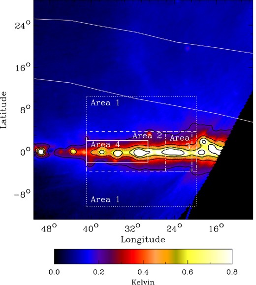
C-BASS 4.76-GHz intensity map using data taken in 2012 January and February showing a region in the first Galactic quadrant. The data are at Nside = 256 and FWHM of 44 arcmin. The white dashed rectangles highlight the four regions, used in this analysis and the white solid curved lines delineate the northern part of the Gould Belt. The empty map region, bottom-right, is due to an absence of C-BASS North data below declination = −30°; this area will be mapped by C-BASS South observations in the future. The colour bar scale is in kelvin and the black contours are spaced at 0.2 K intervals.
The four Galactic plane regions investigated in this work.
| Area | Long. (°) | Lat. (°) | Motivation |
|---|---|---|---|
| 1 | 20–40 | −10 → −4 and 4 → 10 | Synchrotron dominated |
| 2 | 20–40 | −4 → 4 | The RRL data region |
| 3 | 21–26 | −4 → 4 | Typical diffuse region |
| 4 | 30–39 | −2 → 2 | AME region |
| Area | Long. (°) | Lat. (°) | Motivation |
|---|---|---|---|
| 1 | 20–40 | −10 → −4 and 4 → 10 | Synchrotron dominated |
| 2 | 20–40 | −4 → 4 | The RRL data region |
| 3 | 21–26 | −4 → 4 | Typical diffuse region |
| 4 | 30–39 | −2 → 2 | AME region |
2.2 Ancillary data
We have compared the C-BASS maps with the all-sky maps at other frequencies listed in Table 3. We will now briefly discuss each data set in turn. All maps were used in healpix format. Those maps that were originally in a different format were converted to healpix using a nearest-neighbour pixel interpolation. The maps were first smoothed to a common 1° resolution, assuming that the original survey beams were Gaussian with the FWHM specified in Table 3. Depending on the application, the maps were resampled as required to healpixNside = 256 (13.7 arcmin pixels) or Nside = 64 (55 arcmin pixels).
The data used in this paper alongside their frequency, FWHM, healpixNside, calibration uncertainty, average thermal noise (in mK Rayleigh–Jeans unless stated otherwise) and reference. The two bottom rows are derived component separation products.
| Survey | ν | (GHz) | Res. | (arcmin) | Nside | Calibration (per cent) | σ | Reference | ||
|---|---|---|---|---|---|---|---|---|---|---|
| Haslam | 0 | .408 | 51 | 512 | 10 | 700 | Haslam et al. (1982) | |||
| RRLs | 1 | .4 | 14 | .8 | 512 | 15 | 5 | Alves et al. (2012) | ||
| Reich | 1 | .420 | 35 | 512 | 10 | 140 | Reich & Reich (1986) | |||
| Jonas | 2 | .3 | 20 | .0 | 256 | 5 | 30 | Jonas et al. (1998) | ||
| C-BASS | 4 | .76 | 43 | .8 | 256 | 5 | 6 | King et al. (2010) | ||
| WMAP | 22 | .8 | 49 | 512 | 0 | .2 | 0 | .04 | Bennett et al. (2013) | |
| WMAP | 33 | .0 | 40 | 512 | 0 | .2 | 0 | .04 | Bennett et al. (2013) | |
| WMAP | 40 | .7 | 31 | 512 | 0 | .2 | 0 | .04 | Bennett et al. (2013) | |
| WMAP | 60 | .7 | 21 | 512 | 0 | .2 | 0 | .04 | Bennett et al. (2013) | |
| WMAP | 93 | .5 | 13 | 512 | 0 | .2 | 0 | .03 | Bennett et al. (2013) | |
| Planck | 28 | .4 | 32 | .65 | 1024 | 0 | .4 | 0 | .009 | Planck Collaboration I (2014) |
| Planck | 44 | .1 | 27 | .92 | 1024 | 0 | .4 | 0 | .009 | Planck Collaboration I (2014) |
| Planck | 70 | .4 | 13 | .01 | 1024 | 0 | .4 | 0 | .008 | Planck Collaboration I (2014) |
| Planck | 143 | 7 | .04 | 2048 | 0 | .4 | 0 | .0006 | Planck Collaboration I (2014) | |
| Planck | 353 | 4 | .43 | 2048 | 0 | .4 | 0 | .0003 | Planck Collaboration I (2014) | |
| Planck | 545 | 3 | .80 | 2048 | 7 | 0 | .0001 | Planck Collaboration I (2014) | ||
| Planck | 857 | 3 | .67 | 2048 | 7 | 0 | .000 06 | Planck Collaboration I (2014) | ||
| COBE-DIRBE | 1249 | 37 | .1 | 1024 | 13 | .5 | 0 | .5 MJy sr−1 | Hauser et al. (1998) | |
| COBE-DIRBE | 2141 | 38 | .0 | 1024 | 10 | .6 | 32 | .8 MJy sr−1 | Hauser et al. (1998) | |
| COBE-DIRBE | 2997 | 38 | .6 | 1024 | 11 | .6 | 10 | .7 MJy sr−1 | Hauser et al. (1998) | |
| Derived | ||||||||||
| MEM | 22 | .8 | 60 | 128 | – | – | Bennett et al. (2013) | |||
| MCMC | 22 | .8 | 60 | 64 | – | – | Bennett et al. (2013) |
2.2.1 Low-frequency data
We use the Haslam et al. (1982) 408-MHz, Reich & Reich (1986) 1.42-GHz, and Jonas et al. (1998) 2.326-GHz radio maps to provide additional low-frequency information on synchrotron/free–free emission. The Haslam data are used in their unfiltered form, so point sources and striations are still present. These data, alongside the Jonas et al. (1998) data are also used to determine the spectral index between 0.408 and 4.76 GHz outside of the Galactic plane. The Jonas et al. (1998) data only cover the southern sky (−83° < δ < 13°) but fortunately the survey extends to the Galactic plane region under investigation in this work.
Haslam et al. (1982) estimate an uncertainty of 3 K in their global zero level. Although the true random noise is far less than this, striations present in the data are typically 0.5 K and worsen to 3 K in some regions, so we take 3 K as a conservative local uncertainty in the pixel values.
The temperature scale of the 1.420 GHz map is problematic, as extensively discussed by Reich & Reich (1988). The map is nominally on the full-beam scale. Because of the near-sidelobe response within 3| $_{.}^{\circ}$|5, fluxes of point sources obtained by fitting a Gaussian to the central lobe of the beam are expected to be underestimates, and this may be corrected by converting to a ‘main-beam’ brightness temperature. Based on the observed beam profile, this correction was expected to be about 1.25 ± 0.15; however, Reich & Reich (1988) find 1.55 ± 0.08 from direct observations of calibrators, so either the measured beam area or the original temperature scale is in error by around 24 per cent. In our application, we multiplied the data by the empirically deduced correction factor of 1.55. We too find this factor to be consistent with our calibration observations of Barnard's Loop (Section 3). We assign a 10 per cent uncertainty, mainly due to the unquantified variation of the temperature scale with the angular size of the source. We note that Reich & Reich (1988) estimate a full-to-main beam factor of 1.04 ± 0.05 for the 0.408 GHz survey, so it suffers much less from this ‘pedestal’ effect.
To allow for scanning artefacts in the 1.42 GHz maps, we use a conservative local uncertainty of 0.5 K equal to the original estimate of the zero-level uncertainty.
2.2.2 High-frequency data
We use the Planck and WMAP 9-year data to help constrain the spectral form of AME. The WMAPK-band data are specifically used to determine the ratio of AME to total emission between 5 and 23 GHz. The WMAP thermal noise in each healpix pixel (σ) was calculated using the relation (Bennett et al. 2013) |$\sigma = \sigma _{0}/\sqrt{N_{{\rm {obs}}}}$|, where Nobs is the map hit count and σ0 is the thermal noise per sample. Therefore, the rms thermal noise values listed in Table 3 for WMAP are average values across the sky. The Planck 100 and 217 GHz maps were not used as these data include unwanted and significant contributions from the CO lines (Planck Collaboration XIII 2014).
An additional 3 per cent uncertainty was assigned to both the WMAP and Planck data, as in Planck Collaboration XX (2011), to account for residual beam asymmetries after smoothing. Both WMAP and Planck have unblocked and severely underilluminated apertures to reduce sidelobes to extremely low levels, and so the difference between the antenna temperature and full-beam brightness temperature scale is less than 0.5 per cent [in the case of WMAP, the data are corrected for far sidelobe contamination and the corrections from the WMAP ‘main-beam’ to the C-BASS full-beam are less than 0.6 per cent (Jarosik et al. 2007)], and we have not made any correction in this analysis.
We use the COBE-DIRBE band 8, 9 and 10 data to help constrain the spectral form of thermal dust emission. The COBE-DIRBE data used are the Zodi-Subtracted Mission Average data (Hauser et al. 1998).
2.2.3 Free–free templates
At low Galactic latitudes (|b| < 4°), the intensities of the diffuse free–free and synchrotron emission are comparable at gigahertz frequencies. We separate the synchrotron and free–free contributions to total emission in the Galactic plane at 5 GHz; to do this, a free–free emission template was required as well as the C-BASS data. Free–free emission is unpolarized and characterized by a spectral index of β ≈ −2.1 (Dickinson, Davies & Davis 2003; Gold et al. 2009), for optically thin regions. At high frequencies (≈ 90 GHz), the free–free spectral index will steepen (Draine 2011) to −2.14 due to the Gaunt factor, which accounts for quantum mechanical corrections, which become important at higher frequencies.
The source of the diffuse Galactic free–free emission is the WIM, with its intensity proportional to the emission measure (EM), given by EM = ∫(ne)2 dl, where ne is the electron density. The WIM also radiates Hα recombination lines, including the optical Balmer-alpha line (656.28 nm) and high-n radio recombination lines (RRLs) whose strength also depends on the EM. As a result, Hα lines can be used to calculate free–free emission intensities provided the electron temperature is known. However, Hα lines are not satisfactory free–free tracers in the Galactic plane: dust absorption along the line of sight of the Hα lines (which needs to be corrected for throughout the Galaxy) reaches a maximum in the plane due to the increased density of dusty star-forming regions. RRLs from ionized hydrogen provide an absorption-free alternative for tracing free–free emission in the Galactic plane (Alves et al. 2012). We derive the free–free template used in this analysis from RRL data constructed from the HI Parkes All-Sky Survey (Barnes et al. 2001).
The RRL data have a beam FWHM of 14.8 arcmin, and have thermal noise and calibration uncertainties of 5 mK and 15 per cent, respectively. The RRL data (Alves et al. 2012) cover 20° < l < 40°, −4° < b < 4° and were used by Alves et al. to produce a free–free emission template from the data by using an average electron temperature of 6000 K across the whole region. This average value carries a large uncertainty (±1000 K), as it does not account for the presence of warmer and cooler regions. This uncertainty is the dominant factor in the 15 per cent uncertainty assigned to the free–free template.
For this analysis, the RRL data provide our free–free template of choice. As this is a novel approach to deriving free–free templates, we find it illuminating to compare the RRL-derived result with those from WMAP. All-sky free–free models are available from the WMAP 9-year product release constructed using a maximum entropy method (MEM) and Markov Chain Monte Carlo (MCMC) simulation (ADS/Sa.WMAP#K_mem_freefree_9yr_v5.fits and ADS/Sa.WMAP#mcmc_fs_k_freefree_temp_9yr_v5.fits). The MCMC free–free model (Gold et al. 2009) at 22.8 GHz used in this work (‘model f’) fits the total emission model for each pixel as a sum of a power law with a free spectral index parameter for synchrotron emission, a fixed-index power law for the free–free emission, a CMB term, a power law with free spectral index for the thermal dust emission and a theoretical spinning dust curve with amplitude. The MEM free–free model at 22.8 GHz is a similar spectral pixel-by-pixel fit, which uses Bayesian priors for pixels where the data do not constrain the parameters very well (see Gold et al. 2009 for details).
3 DATA VALIDATION
We have considered the effect of pointing errors, absolute intensity calibration, colour (bandpass) corrections and atmospheric opacity on the C-BASS temperature scale, but the dominant error is the uncertainty on the aperture efficiency, which we estimate at 5 per cent. To assess the consistency of the C-BASS temperature scale, we compare C-BASS data with other radio surveys. We focus on Barnard's Loop, an H ii shell within the Orion complex (Heiles et al. 2000). This region is known to be dominated by optically thin free–free emission at these frequencies, which allows us to use the well-defined spectral index to compare data at a range of frequencies. Fig. 2 shows Barnard's Loop in Hα Balmer line emission and in 4.76 GHz radio continuum as seen by C-BASS North. The boxed region shows the specific area selected for analysis in Fig. 3. The close morphological similarity indicates that free–free emission from warm ionized gas dominates.
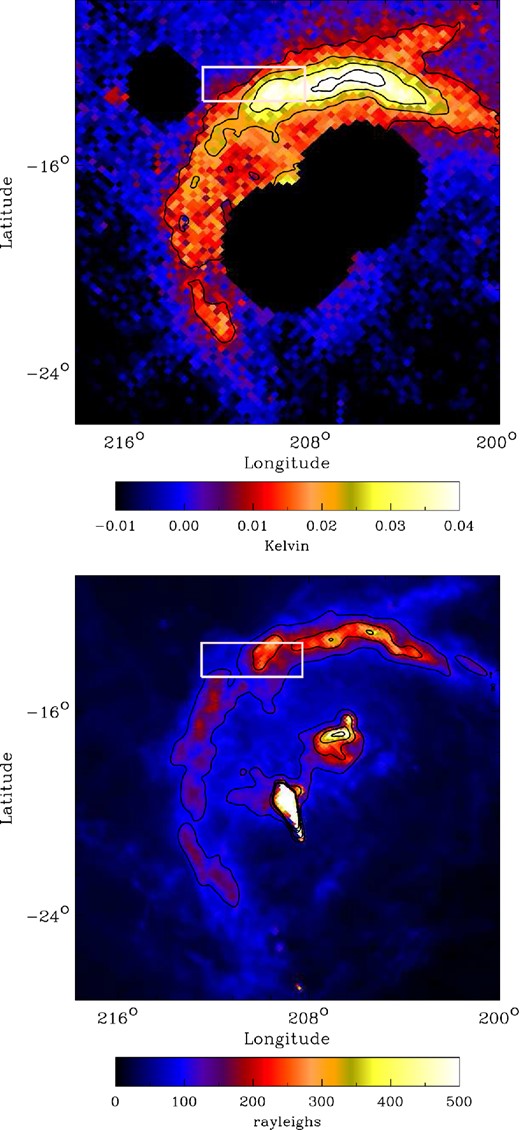
Top: Barnard's Loop as seen at 4.76 GHz by C-BASS North. Nside = 256 and FWHM resolution of 0| $_{.}^{\circ}$|73. Orion A, Orion B and NVSS J060746-062303 are masked out. The colour scale is in kelvin and the contours are spaced at 0.01 K intervals. Bottom: Barnard's Loop in Hα emission at healpixNside = 512 and resolution 6.1 arcmin. The colour scale is in rayleighs and the contours spaced at 100 rayleigh intervals between 100 and 500 (Finkbeiner 2003). The morphological similarity between the maps suggests that free–free emission is dominant at 4.76 GHz. The white box encapsulates the region selected for temperature analysis.
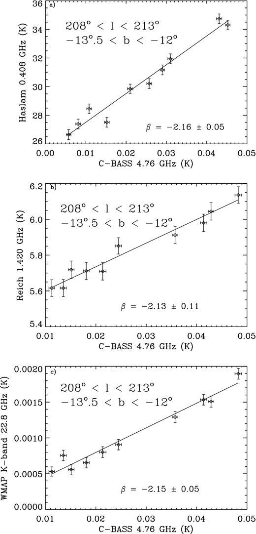
T–T plots of the Barnard's Loop region between 4.76 GHz and (a) 0.408 GHz, (b) 1.42 GHz and (c) 22.8 GHz. The spectral indices confirm a free–free emission-dominated region.
The compact sources Orion A (M42), Orion B and NVSS J060746-062303 have been masked out of the C-BASS image using a diameter 3.5 times the C-BASS FWHM for Orion A and B and 2 times the C-BASS FWHM for NVSS J060746-062303 (see Fig. 2). A smaller mask size could be used for NVSS J060746-062303 as the source is fainter than Orion A or Orion B.
Fig. 3 displays T–T plots using the C-BASS data for Barnard's Loop against Haslam et al. (1982), Reich & Reich (1986) and WMAPK-band data. The T–T plots are made at Nside = 64 to reduce correlations between the pixels – at an FWHM of 1°, this gives <2 pixels per beam.
The error bars in Fig. 3 represent the pixel noise for the respective radio maps calculated using 1000 iteration Monte Carlo simulations. These include the effects of confusion noise (0.8 mK for the C-BASS data), zero-level uncertainties (3 K for the Haslam et al. 1982 and 0.5 K for the Reich & Reich 1986 data), CMB anisotropies (for the WMAP data), healpix smoothing and degrading as well as the rms thermal noise. The CMB anisotropies were simulated using the camb web interface1 (Lewis, Challinor & Hanson 2011) and the standard, pre-set cosmological parameters. It was determined that calibration uncertainty, and not pixel noise, was the dominant source of uncertainty. The uncertainties quoted for the spectral indices are a quadrature combination of the pixel errors and calibration uncertainties associated with each data set.
The 0.408–4.76, 1.42–4.76 and 4.76–22.8 GHz T–T plots in Fig. 3 show linear fits; the reduced χ2 values are 1.9, 0.5 and 1.3 for the 0.408–4.76, 1.42–4.76 and 4.76–22.8 GHz data, respectively. The average spectral index of β = −2.15 ± 0.03 confirms a free–free-dominated spectrum for Barnard's Loop. This spectral index is consistent within 1σ of the expected value (β ≈ −2.12).
The multiplicative factor required to bring C-BASS data to be in perfect agreement with WMAP 22.8 GHz data (assuming all the emission is due to free–free emission) is 0.95 ± 0.05. This validation gives us confidence that there are no significant systematic calibration errors in excess of the 5 per cent calibration error assigned to the preliminary C-BASS data.
4 DIFFUSE EMISSION BETWEEN 0.408 AND 4.76 GHz
The total diffuse Galactic plane radio continuum emission seen at 4.76 GHz is primarily a mixture of free–free and synchrotron emission. Free–free emission is known to have a narrow latitude distribution while synchrotron emission is broader (Alves et al. 2012; Planck Collaboration XXIII 2014). The narrow width of the free–free distribution shown in Section 4.2 suggests that the free–free contribution is negligible compared to the synchrotron contribution at latitudes higher than four degrees. This suggestion is supported by the Hα free–free template (Dickinson et al. 2003), which covers off-plane regions. It is therefore possible to determine the spectral index of synchrotron emission between 0.408 and 4.76 GHz at intermediate and high Galactic latitudes without having to perform any free–free/synchrotron emission separation.
4.1 Intermediate latitude total emission spectral indices
The spectral index of the Galactic synchrotron emission varies significantly, both spatially and with frequency. Strong, Orlando & Jaffe (2011) review results from sky maps between 22 MHz and 23 GHz at intermediate latitudes, finding a steepening in the synchrotron spectrum from β ≈ −2.5 at 0.1 GHz to β ≈ −3 at 5 GHz. Between 0.408 and 3.8 GHz, an index of ≈−2.7 has been estimated in the Galactic plane whereas between 1.42 and 7.5 GHz the spectrum appears to steepen to ≈−3.0 (Platania et al. 1998). Jaffe et al. (2011), Lawson et al. (1987) and Bennett et al. (2003) also discuss the spectral steepening of synchrotron emission in the Galactic plane and it is clear that between 2.3 and 22.8 GHz the spectral index undergoes a steepening from ≈−2.7 to ≈−3.1. Due to the relationship between electron energy distribution N(E) ∝ E δ, and synchrotron spectral index β = −(δ + 3)/2, this spectral index steepening results from a steepening of the cosmic ray electron spectrum. It resembles that expected from synchrotron losses, i.e. a ‘break’ (actually a rather smooth steepening) of 0.5–1 in β assuming a steady state between injection of fresh particles, radiative loss and transport out of the Galaxy (e.g. Bulanov & Dogel 1974; Strong et al. 2011). However, the time-scale for electrons to leave the Galaxy implied by this interpretation is far shorter than the cosmic ray residence time-scales inferred from the presence of spallation product nuclei in the cosmic rays, so in current models (e.g. Orlando & Strong 2013) the steepening is explained by a break in the electron injection energy spectrum; the break due to radiative losses is predicted to occur at a much lower frequency than is actually observed.
The steepening of the synchrotron spectrum at a few GHz is consistent with the measured steepening of the local cosmic ray electron spectrum (Abdo et al. 2009), with δ varying from <2.3 to ≈3 between 1 and 10 GeV (solar modulation prevents accurate measurement of δ much below 1 GeV).
Reich & Reich (1988) observed a steepening along the Galactic plane of the synchrotron β (between 0.408 and 1.420 GHz) with β = −2.86 at (l, b) = (20°, 0°) and β = −2.48 at (l, b) = (85°, 0°). Peel et al. (2012) comment on the lack of flatter-spectrum (β ≈ −2.7) emission at high latitudes between 2.3 and 30 GHz, in contrast to the Galactic plane. Conversely, the most sophisticated models of cosmic ray propagation in the Galaxy to date (Orlando & Strong 2013) predict variations in β of no more than 0.1 between different directions, e.g. between the plane and higher latitudes. These models are explicitly of the large-scale diffuse emission only, and so will omit any spectral variations caused by features on sub-kpc scales, including the radio ‘loops’ that dominate the high-latitude synchrotron emission. These are expected to cause variations in β because they may be sites of particle injection, hence with flatter spectra (as for most supernova remnants) and because they have stronger magnetic fields, so emission at a given frequency is from lower energy electrons (which will also flatten the spectrum). Spectra steeper than the diffuse emission require that they contain old electrons confined by a very low effective diffusion coefficient in magnetic fields much stronger than typical interstellar fields, so that significant in situ radiative losses can occur without compensating particle acceleration. It is also worth noting that the low-latitude regions claimed to show flatter synchrotron spectra are the ones most contaminated by free–free emission, e.g. the Cygnus X region at l = 75°–86°.
Fig. 4 shows T–T plots of semicorrelated pixels (6 pixels per beam), which were made in the off-plane latitude range of 4° < |b| < 10° with no masking of specific regions. We expect this region to be dominated by synchrotron emission between 0.408/1.420and 4.76 GHz. The positive and negative latitude ranges are plotted separately to differentiate between Galactic plane emission and emission from the North Polar Spur and the Gould Belt. The region in Figs 4(b) and (d) encompass part of the Gould Belt and the North Polar Spur. The variation in synchrotron spectral index across the positive latitude range results in a bulged point distribution in Fig. 4(b) between 0.12 and 0.16 K on the x-axis.
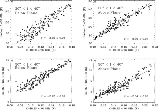
Top row: T–T plots between 0.408 and 4.76 GHz for (a) −10° < b < −4° (Below plane) and (b) 10° > b > 4° (Above plane). Bottom row: T–T plot for 1.420 and 4.76 GHz for (c) −10° < b < −4° and (d) 10° > b > 4°. The off-plane spectral indices between 0.408 and 4.76 GHz can be seen to range between −2.67 and −2.72.
The mean spectral indices shown in Fig. 4 are summarized in Table 4 and range between β = −2.64 and −2.72. The weighted mean spectral indices between 0.408–4.76 and 1.420–4.76 GHz are −2.67 ± 0.04 and −2.68 ± 0.06, respectively. These results are consistent with, but more accurate than, those in the literature, which typically give an average synchrotron spectral index of ≈−2.7 both within the Galactic plane and away from the radio ‘loops’. The C-BASS data provide a longer lever-arm for constraining spectral indices with uncertainties Δβ < 0.1. The larger uncertainties on the 1.420–4.76 spectral indices are due to the larger uncertainties in the 1.42 GHz survey. We expect the full C-BASS survey to have a significantly reduced uncertainty in its calibration, and in conjunction with other modern surveys such as S-PASS (Carretti et al. 2013) we should be able to constrain the spectral index and possible curvature (steepening/flattening) of the spectrum even more accurately.
The off-plane (4° < |b| < 10°) spectral indices between 0.408/1.420 and 4.76 GHz.
| Long. (°) | Lat. (°) | ν (GHz) | β |
|---|---|---|---|
| 20–40 | −10 → −4 | 0.408–4.76 | −2.65 ± 0.05 |
| 20–40 | 4 → 10 | 0.408–4.76 | −2.69 ± 0.05 |
| 20–40 | −10 → −4 | 1.420–4.76 | −2.72 ± 0.09 |
| 20–40 | 4 → 10 | 1.420–4.76 | −2.64 ± 0.09 |
| Long. (°) | Lat. (°) | ν (GHz) | β |
|---|---|---|---|
| 20–40 | −10 → −4 | 0.408–4.76 | −2.65 ± 0.05 |
| 20–40 | 4 → 10 | 0.408–4.76 | −2.69 ± 0.05 |
| 20–40 | −10 → −4 | 1.420–4.76 | −2.72 ± 0.09 |
| 20–40 | 4 → 10 | 1.420–4.76 | −2.64 ± 0.09 |
4.2 Free-free cleaned maps at 0.408/1.420/4.76 GHz
At low Galactic latitudes (|b| < 4°), the free–free emission cannot be assumed to be negligible; the synchrotron and free–free components need to be separated. Assuming that below 5 GHz only synchrotron and free–free emission are present at a detectable level, synchrotron maps can be formed from the Haslam et al. (1982), Reich & Reich (1986) and C-BASS data using a pixel-by-pixel subtraction of a free–free template of choice. More sophisticated component separation methods, such as parametric fitting, could be used to acquire synchrotron maps but this would require an accurate estimate of the C-BASS zero-level. Therefore, until the full survey is complete, we use simpler methods of component separation.
In Fig. 5, we present two latitude profiles for the RRL, MEM and MCMC free–free templates overplotted on the C-BASS data for the same region. The RRL, MCMC and MEM templates have been scaled to 4.76 GHz using the free–free spectral index of β = −2.1. The free–free profiles all have their baselines subtracted so that the in-plane emissions can be compared without biasing from different survey zero-levels. The baseline level was established using a cosecant (1/sin(|b|)) plus a slope to the |b| < 10° points for each of the curves. We then subtract the slope (offset and gradient) to leave the plane emission. The 1° FWHM maps were resampled at healpixNside = 64 to match the MCMC template. The two latitude profiles average over (a) 21° < l < 26° and (b) the full RRL longitude range 20° < l < 40°. The 21° to 26° longitude range was selected to be a typical bright diffuse region as it contained the fewest bright, compact areas in the C-BASS map. Both profiles span the full RRL latitude range of −4° < b < 4°.
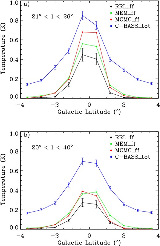
Free–free latitude distribution for |b| < 4° using averaged longitude data from the RRL, MCMC, MEM free–free templates all scaled to 4.76 GHz for the longitude range of (a) 21°–26° and (b) 20°–40°. The maps have been smoothed to 1° resolution and downgraded to healpixNside = 64.
The C-BASS data were used as a ‘testbed’ for these templates and help to identify regions over which they fail to describe the measured emission. The RRL free–free template is systematically lower in temperature than the MEM and MCMC templates because the electron temperature used is 1000 K lower than the 7000 K assumed by WMAP. The RRLs are a more direct free–free measure as they are not subject to the same parameter degeneracies faced by the MCMC and MEM templates but of course are so far only available for |b| < 4° and a limited range of longitudes.
Three synchrotron maps at 0.408, 1.420 and 4.76 GHz were made by subtracting the RRL free–free template from the Haslam et al. (1982), Reich & Reich (1986) and C-BASS maps. The RRL free–free template was scaled to the different frequencies using a single power law with β = −2.1. The synchrotron maps, scaled to 4.76 GHz (using β values given in Table 5), are shown as latitude profiles in Fig. 6. The best-fitting synchrotron spectral indices required to match the 0.408/1.420 GHz latitude profiles with their corresponding 4.76 GHz values are shown in Table 5. The data are shown at healpixNside = 256 so as to fully sample the latitude profile, resulting in correlated pixel errors. The thermal noise is shown as error bars while the average calibration errors (based on a 0.4 K signal) are shown in the legend. Fig. 6(a) averages over the 21° to 26° longitude range while Fig. 6(b) averages over the entire 20° to 40° longitude range. As in Fig. 5, the synchrotron curves are shown after the subtraction of their zero-levels. Both Figs 6(a) and (b) display the broad peaks typically associated with synchrotron emission. Although one average synchrotron spectral index is clearly a good approximation across the |b| = 4° latitude range, small-scale differences are seen between the curves. A full analysis of the intensity and polarization data sets will reveal which of these differences are physically interesting.
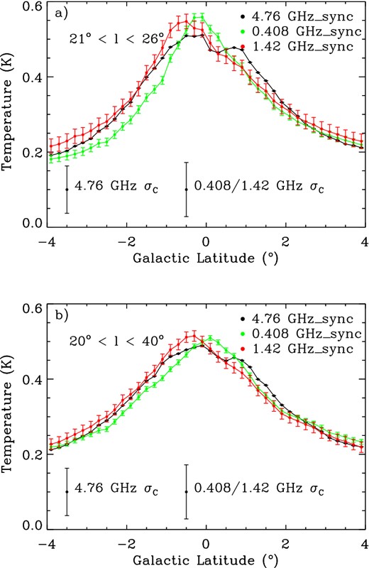
Latitude profiles of Galactic synchrotron emission for |b| < 4° using averaged longitude data from the RRL free–free-subtracted Haslam et al. (1982), Reich & Reich (1986) and C-BASS data, all scaled to 4.76 GHz for the longitude range of (a) 21°–26° and (b) 20°–40° (see Table 5). The maps have been downgraded to healpixNside = 256 and are smoothed to 1° resolution. The thermal noise is shown as error bars on the data points while the calibration uncertainty (based on a 0.4 K signal) are shown at the bottom of each panel. The broad profile expected for synchrotron emission is clearly visible.
The Galactic plane synchrotron spectral indices as determined using synchrotron maps formed using the RRL free–free templates.
| Long. (°) | ν range | β |
|---|---|---|
| 21–26 | 0.408–4.76 | −2.59 ± 0.08 |
| 21–26 | 1.420–4.76 | −2.69 ± 0.17 |
| 20–40 | 0.408–4.76 | −2.56 ± 0.07 |
| 20–40 | 1.420–4.76 | −2.62 ± 0.14 |
| Long. (°) | ν range | β |
|---|---|---|
| 21–26 | 0.408–4.76 | −2.59 ± 0.08 |
| 21–26 | 1.420–4.76 | −2.69 ± 0.17 |
| 20–40 | 0.408–4.76 | −2.56 ± 0.07 |
| 20–40 | 1.420–4.76 | −2.62 ± 0.14 |
These in- and off-plane results confirm a synchrotron spectral index of −2.72 < β < −2.64 between 0.408 and 4.76 GHz for −10° < b < 10°. Once again, no significant spectral steepening of the synchrotron spectral index is observed and the values are in agreement with the expected index of −2.7.
At 1.5 GHz, diffuse Galactic emission has been shown to be roughly 30 per cent free–free and 70 per cent synchrotron emission (Platania et al. 1998). The ratio between free–free and synchrotron emission at 4.76 GHz can now be determined using the derived latitude distributions of the 4.76 GHz pure synchrotron map. Fig. 7 shows latitude profiles across −4° < b < 4° for the total 4.76 GHz emission as measured by C-BASS, the RRL free–free map scaled to 4.76 GHz using β = −2.1 and the 4.76-GHz pure synchrotron map. Extrapolating our results to 1.5 GHz, the fraction of synchrotron emission present is 70 ± 10 per cent while at 4.76 GHz it was found to be 53 ± 8 per cent for 20° < l < 40°, −4° < b < 4°.
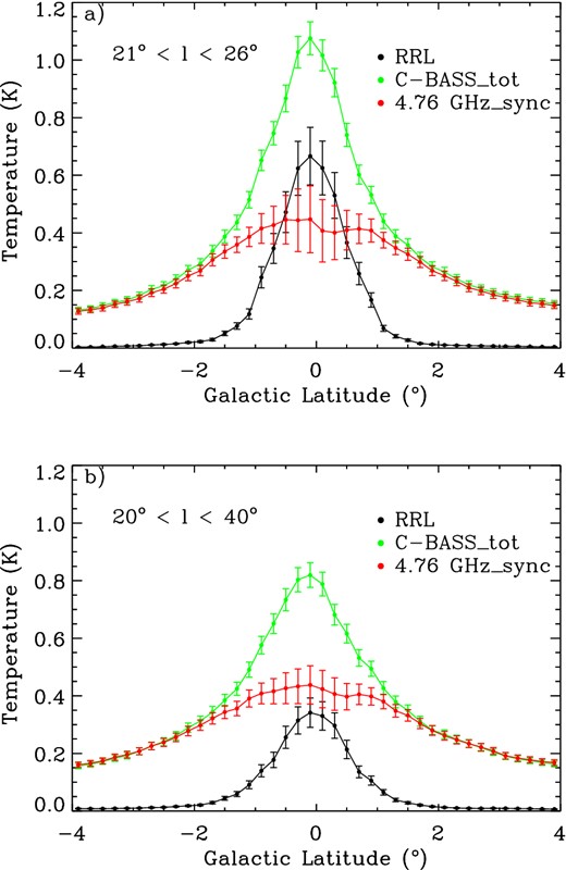
Total emission latitude distribution for |b| < 4° using RRL and C-BASS data all at 4.76 GHz with the longitude data averaged between (a) 21° and 26° and (b) 20° and 40°. The maps have been downgraded to healpixNside = 256 and are smoothed to 1° resolution.
5 IDENTIFICATION OF ANOMALOUS EMISSION AT 22.8 GHz
At the WMAPK-band frequency of 22.8 GHz, diffuse emission in the Galactic plane is a combination of free–free, synchrotron and AME.The favoured emission mechanism for AME is electric dipole radiation from spinning dust grains (e.g. Draine & Lazarian 1998; Davies et al. 2006; Planck Collaboration XX 2011). AME has been readily identified in dark clouds and molecular clouds (Watson et al. 2005; Casassus et al. 2008; AMI Consortium et al. 2011; Vidal et al. 2011). However, it is also present throughout the Galactic plane and adds to the complexity of component separation of CMB data (Planck Collaboration XX 2011; Planck Collaboration XV 2014). For example, with only full-sky data at 1.4 and 22.8 GHz, the presence of AME, which peaks in flux density at ∼ 30 GHz (Planck Collaboration XX 2011), will appear only as a flattening of the total-emission power law. Here, we use the preliminary C-BASS data to help characterize the synchrotron signal and so detect the presence of AME. The 4.76-GHz C-BASS data provides a higher frequency measure of the synchrotron emission, which is uncontaminated by AME, and can thus be used in combination with 22.8 GHz data to separate the different spectral components.
5.1 Diffuse AME
For this analysis, the following three regions were chosen for their combination of bright diffuse and compact regions: 30° < l < 33°, 33° < l < 36° and 36° < l < 39° for −2° < b < 2°. In this section, we will use T–T plots to probe the diffuse emission while in the next section will use spectral energy distributions (SEDs) to probe the compact regions.
At 22.8 GHz, the synchrotron contribution is negligible at low Galactic latitudes, away from bright supernova remnants. This is apparent from scaling the 0.408 GHz map to 22.8 GHz using β = −2.7 as the scaled Haslam et al. (1982) signal is, on average, an order of magnitude lower than the WMAP intensity signal. Therefore, the spectral index determined from the WMAP–C-BASS T–T plots is expected to be dominated by free–free emission (β ≈ −2.1). If spectral indices less than −2.1 are found, the flattening would indicate the presence of AME at 22.8 GHz.
Fig. 8 shows T–T plots between 4.76 and 22.8 GHz for those three regions. The goodness-of-fit for all three plots are fairly poor as spatial variations within the beam result in outliers. The pixel uncertainties shown on the plots, are quite small as, on the plane, the thermal noise is negligible. Therefore, the spatial variations within the beam dominate the formal spectral index errors, which also take into account the survey calibration errors as well as the plotted thermal errors.
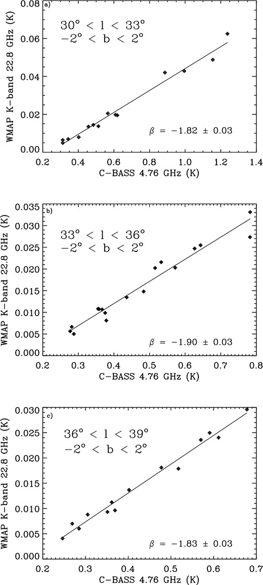
T–T plot between 4.76 and 22.8 GHz for Galactic latitude −2° < b < 2° and (a) Galactic longitude 30° < l < 33°, (b) Galactic longitude 33° < l < 36° and (c) Galactic longitude 36° < l < 39°. All maps have been downgraded to Nside = 64 and smoothed to 1° resolution. The presence of AME between 4.76 and 22.8 GHz is implied by the flatter (β > −2.0) spectral indices.
For the regions shown in Figs 8(a), (b) and (c), the percentage of the total emission that can be explained as AME is calculated to be 37 ±5, 29 ±6 and 37 ± 8 per cent, respectively. This is comparable to the 48 ±5 per cent AME to total emission ratio that was found in the inner Galaxy using Planck data (Planck Collaboration XXIII 2014). This calculation provides a 7σ, 4σ and 4σ detection of AME for the three −2° < b < 2° and 30° < l < 39° sub-regions. These result are summarized in Table 6 for a frequency of 22.8 GHz. The table also contains the ratios of AME to free–free emission, which show the AME to be roughly half of the free–free magnitude.
The total emission spectral indices between 4.76 and 22.8 GHz and the AME to total emission and AME to free–free emission ratios at 22.8 GHz for −2° < b < 2°.
| Long. | βtot | AME/tot | AME/ff |
|---|---|---|---|
| (°) | (per cent) | (per cent) | |
| 30–33 | −1.82 ± 0.03 | 37 ± 5 (7σ) | 60 ± 13 (4σ) |
| 33–36 | −1.90 ± 0.03 | 29 ± 5 (4σ) | 41 ± 12 (3σ) |
| 36–39 | −1.83 ± 0.03 | 37 ± 8 (4σ) | 58 ± 12 (4σ) |
| Long. | βtot | AME/tot | AME/ff |
|---|---|---|---|
| (°) | (per cent) | (per cent) | |
| 30–33 | −1.82 ± 0.03 | 37 ± 5 (7σ) | 60 ± 13 (4σ) |
| 33–36 | −1.90 ± 0.03 | 29 ± 5 (4σ) | 41 ± 12 (3σ) |
| 36–39 | −1.83 ± 0.03 | 37 ± 8 (4σ) | 58 ± 12 (4σ) |
5.2 Spectral Energy Distributions (SEDs)
Three prominent low-latitude extended sources, centred at (l, b) = (30| $_{.}^{\circ}$|8, − 0| $_{.}^{\circ}$|3), (34| $_{.}^{\circ}$|8, − 0| $_{.}^{\circ}$|5), (37| $_{.}^{\circ}$|8, − 0| $_{.}^{\circ}$|2), can be seen within Area 4 demarcated on Fig. 1. These are W43 (a complex H ii region), W44 (an SNR) and W47 (a complex H ii region), respectively. To determine whether the presence of AME calculated from the T–T plots may be explained by excess emission due to these regions, we can calculate the SEDs for these individual complexes.
Flux densities for complex extended sources are best determined through aperture photometry. This technique measures the integrated flux without the need to fit Gaussians. Aperture photometry involves forming an inner aperture centred on the source centre and an outer annulus over the source background.
SEDs of W43, W44 and W47 are shown in Fig. 9. Zoomed-in plots of the AME spectrum are included within each SED to highlight the region of interest. To determine the source flux densities, the maps were downgraded to healpixNside = 256 when necessary. Aperture photometry was carried out and the inner aperture size was chosen to be 60 arcmin in radius with the outer annulus spanning from 80 to 100 arcmin so as to match the analysis in Planck Collaboration XV (2014). The flux densities for W43, W44 and W47 are listed in Table 7. The uncertainties are the quadrature addition of the calibration and the background subtraction uncertainties.
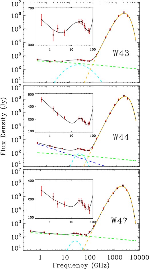
From top to bottom panel: SEDs for (l, b) = (30| $_{.}^{\circ}$|8, −0| $_{.}^{\circ}$|3), (l, b) = (34| $_{.}^{\circ}$|8, −0| $_{.}^{\circ}$|5) and (l, b) = (37| $_{.}^{\circ}$|8, −0| $_{.}^{\circ}$|2). Flux densities were determined via aperture photometry using the Haslam et al. (1982), Reich & Reich (1986), Jonas et al. (1998), C-BASS, WMAP, Planck and COBE-DIRBE data. All the maps were smoothed to 1° resolution and downgraded to healpixNside = 256. The solid black line represents the total emission model while the yellow dashed line represents the thermal dust emission model, the light blue dashed line represents AME, the dark blue dashed line represent synchrotron and the dashed green line represents free–free emission. All three sources clearly show the presence of AME in the form of a bump centred around 30 GHz.
The colour-corrected flux densities for the W43, W44 and W47 acquired using aperture photometry with a 60 arcmin inner aperture radius.
| Frequency (GHz) | Flux Density (Jy) | ||
|---|---|---|---|
| W43 | W44 | W47 | |
| (30| $_{.}^{\circ}$|8, −0| $_{.}^{\circ}$|3) | (34| $_{.}^{\circ}$|8, −0| $_{.}^{\circ}$|5) | (37| $_{.}^{\circ}$|8, −0| $_{.}^{\circ}$|2) | |
| 0.408 | 534 ± 65 | 570 ± 68 | 271 ± 46 |
| 1.420 | 381 ± 33 | 349 ± 27 | 216 ± 22 |
| 2.3 | 440 ± 32 | 267 ± 22 | 168 ± 19 |
| 4.76 | 400 ± 26 | 216 ± 17 | 166 ± 15 |
| 22.8 | 509 ± 26 | 211 ± 17 | 188 ± 16 |
| 28.4 | 502 ± 26 | 203 ± 16 | 184 ± 16 |
| 33.0 | 490 ± 25 | 189 ± 15 | 170 ± 15 |
| 40.7 | 467 ± 23 | 178 ± 14 | 159 ± 14 |
| 44.1 | 435 ± 22 | 164 ± 14 | 148 ± 13 |
| 60.7 | 419 ± 21 | 159 ± 14 | 151 ± 13 |
| 70.4 | 408 ± 22 | 160 ± 14 | 132 ± 14 |
| 93.5 | 551 ± 30 | 243 ± 21 | 231 ± 22 |
| 143 | 1213 ± 80 | 1231 ± 61 | 610 ± 71 |
| 353 | (2.20 ± 0.17) × 104 | (2.19 ± 0.13) × 104 | (1.18 ± 0.15) × 104 |
| 545 | (8.46 ± 1.1)× 104 | (8.55 ± 1.1) × 104 | (4.48 ± 0.74)× 104 |
| 857 | (3.49 ± 0.43)× 105 | (3.61 ± 0.41) × 105 | (1.72 ± 0.26) × 105 |
| 1249 | (8.67 ± 1.2) × 105 | (9.10 ± 1.2) × 105 | (3.94 ± 0.63) × 105 |
| 2141 | (1.77 ± 0.21) × 106 | (1.92 ± 0.21) × 106 | (6.61 ± 0.091) × 105 |
| 2997 | (9.77 ± 1.4) × 105 | (1.10 ± 0.15) × 106 | (3.20 ± 0.5) × 105 |
The synchrotron spectral behaviour was modelled as a power law, with an amplitude and spectral index β. The free–free emission has a well-determined spectral shape with just the amplitude (EM). The Gaunt factor (gff) is required to take into account quantum mechanical contributions and the electron temperature is assumed to have a typical value of 7000 K (Draine 2011). The thermal dust was assumed to behave as a grey body with dust temperature and emissivity index. The amplitude is normalized using the 250-μm optical depth (τ250). The AME component was fitted as a parabola in log S–log ν (Bonaldi et al. 2007) where m60 is a free parameter, which represents the slope of the parabola at 60 GHz, νpeak is the AME peak frequency. This method requires no prior information on the physical properties of dust grains responsible for the AME.
Colour corrections were applied to the WMAP, Planck and COBE-DIRBE data within the least-squares fitting routine. This enables the model-fitted spectrum to be used as the source spectrum required for the colour correction. The WMAP colour corrections are calculated by weighting the bandpass at a lower, central and upper limit, these limits and their weights are given in Bennett et al. (2013). The idl code used to compute the Planck Low Frequency Instrument (LFI) and High Frequency Instrument (HFI) colour correction were taken from the Planck external tools repository (Planck Collaboration V 2014; Planck Collaboration IX 2014)2 and the COBE colour correction tables are given on the LAMBDA website (ADS/Sa.COBE#DIRBE_COLOR_CORRECTION_TABLES>ASC).
The W43 data are well fitted by the total emission model with a reduced χ2 of 1.0. The AME peak, the largest difference between the total emission model and the free–free + synchrotron + thermal dust emission model, is identified at the 4.4σ level. The large uncertainty on the m60 parameter (see Table 8) comes from the fact that few of the measurements are characterized by this parameter. The W44 data are the least well fitted by the total emission model with a reduced χ2 of 2.6. This is due to a slightly poorer fit between the three COBE-DIRBE points and the grey body model of thermal dust. If the reduced χ2 is recalculated using the full data set to determine the model parameters but leaving out the COBE-DIRBE points to determine the goodness-of-fit, a value of 1.9 is found. This is assuming the full 10 degrees of freedom. The AME peak is identified at the 3.1σ level. The W47 data are well fitted by the total emission model with a reduced χ2 of 0.6. The AME peak is identified at the 2.5σ level. It should be noted that the EM fitted values are only effective EM values for the 1° radius inner aperture.
The analysis was repeated with the 4.76-GHz C-BASS point excluded from the fits to quantify the impact of the additional constraint. Table 8 shows the fitted parameters for W43, W44 and W47 with and without the C-BASS data point included in the fit. It can be seen that the lack of 4.76 GHz data increases the uncertainty on the synchrotron spectral index, from 0.08 to 0.09, for W44 and the uncertainty associated with the free–free EM of W43. The 0.01 variation in the W44 synchrotron spectral index may in fact represent an actual value shift after the inclusion of additional synchrotron information. The AME flux decreases by 17 per cent for W43, increases by 7 per cent for W44 and 8 per cent for W47 and the uncertainties on the dust temperatures of W44 and W47 triple. The AME peak frequencies for W44 and W47 are seemingly unaffected by the C-BASS data point, while the W43 AME peak frequency has a lower uncertainty when the C-BASS point is included.
The W43, W44 and W47 fitted total emission parameters with and without the C-BASS data point.The parameters, from top to bottom, represent the reduced chi squared, the spectral index of synchrotron emission, the dust temperature, the spectral index of thermal dust emission, the spinning dust slope parameter, the peak frequency of spinning dust emission, the EM, the optical depth at 250 μm and the AME peak flux density.
| W43 | W44 | W47 | ||||
|---|---|---|---|---|---|---|
| Parameter | With | Without | With | Without | With | Without |
| Reduced χ2 | 1.0 | 1.0 | 2.6 | 2.8 | 0.7 | 0.8 |
| βsync | – | – | −2.57 ± 0.08 | −2.56 ± 0.09 | – | – |
| Td (K) | 23.3 ± 0.5 | 23.3 ± 0.6 | 25.2 ± 0.5 | 25.3 ± 1.5 | 19.9 ± 0.4 | 21.3 ± 1.5 |
| βthermal | 1.78 ± 0.06 | 1.77 ± 0.05 | 1.69 ± 0.05 | 1.69 ± 0.07 | 1.91 ± 0.07 | 1.80 ± 0.07 |
| m60 | 1 ± 0.2 | 2 ± 1 | 4 ± 2 | 5 ± 2 | 5 ± 4 | 7 ± 6 |
| νpeak (GHz) | 23 ± 3 | 22 ± 9 | 27 ± 3 | 28 ± 2 | 25 ± 5 | 26 ± 6 |
| EM | 97 ± 8 | 77 ± 7 | 24 ± 1 | 24 ± 2 | 46 ± 2 | 49 ± 3 |
| τ250 | 0.011 ± 0.0006 | 0.011 ± 0.002 | 0.009 ± 0.0007 | 0.007 ± 0.0008 | 0.009 ± 0.0009 | 0.007 ± 0.0006 |
| AME peak flux (Jy) | 218 ± 29 | 186 ± 41 | 90 ± 13 | 96 ± 14 | 50 ± 11 | 54 ± 4 |
The level of improvement seen when the C-BASS point is included in the fit is clearly strongly dependent on the region under investigation. In these three regions, it turns out that the C-BASS data point is in excellent agreement with the fitted spectral model and therefore it has a minimal impact. Furthermore, these regions benefit from the use of the 2.3-GHz data point. Also, from Fig. 9 it can be seen that the W43 AME model parabola is far wider than the W44 or W47 parabola. The width of the W43 AME peak even when the C-BASS data point is included in the fit suggests that the models are still not well enough constrained. Data between 4.76 and 22.8 GHz would be of great use for this spectral fit, for example the 11, 13, 17 and 19 GHz measurements of the QUIJOTE experiment (López-Caniego et al. 2014).
5.2.1 Contribution from UCHII
The Planck Collaboration have previously noted the possibility of AME within W43 (Planck Collaboration XV 2014). For their analysis, they used aperture photometry to determine the flux density values and they measured a σAME of 8.6; however, they assign a 36 per cent contribution to the total emission to emission from nearby ultracompact H ii (UCHII) regions. Therefore, we will now consider the possible contribution of UCHII regions to the detection of diffuse AME.
If a UCHII region, optically thick at 5 GHz, were to be positioned within one of the source regions, this would result in what would appear to be excess emission at higher frequencies where the UCHII region becomes optically thin. To ensure that the excess emission seen around 30 GHz in the W43, W44 and W47 SEDs is due to AME, the sources must be checked for nearby optically thick UCHII regions.
In the Planck Collaboration XV (2014) paper, the method of Dickinson (2013) and Wood & Churchwell (1989) was employed. This method uses the fact that UCHII regions generally possess IRAS colours (brightness ratios) of |$\log _{10} (\frac{S_{60}}{S_{12}}) \ge 1.30$| and |$\log _{10} (\frac{S_{25}}{S_{12}} ) \ge 0.57$|.
Recently, a new catalogue of UCHII regions at 5 GHz has become available via the CORNISH (Co-Ordinated Radio ‘N’ Infrared Survey for High mass star formation) VLA survey. The CORNISH survey covers the 10° < l < 65°, |b| < 1° region of the Galactic plane at a resolution of 1.5 arcsec and rms noise of 0.4 mJy per beam (Purcell et al. 2013). Using the online catalogue (Hoare et al. 2012), several possible UCHII regions were found within a 0| $_{.}^{\circ}$|5 radius of W43 and W47 and their flux densities and optical depth values are shown in Table 9. The flux densities and FWHMs are listed in the CORNISH catalogue and used to calculate the brightness temperature, which in turn are used to calculate the optical depth at 5 GHz.
The 5-GHz flux density, FWHM, brightness temperature and 5-GHz optical depth values of the UCHII regions found within 0| $_{.}^{\circ}$|5 of W43, W44 and W47 using the CORNISH 5 GHz catalogue.
| Source | S (mJy) | FWHM (arcsec) | Tb (K) | τ5 |
|---|---|---|---|---|
| W43 | ||||
| G030.8662+00.1143 | 325 | 3.1 | 1667 | 0.20 |
| G030.7532−00.0511 | 302 | 3.3 | 1363 | 0.15 |
| G031.1596+00.0448 | 24 | 2.4 | 206 | 0.02 |
| G030.7197−00.0829 | 969 | 4.6 | 2250 | 0.25 |
| G030.6881−00.0718 | 467 | 10.8 | 195 | 0.02 |
| G030.7661−00.0348 | 88 | 3.3 | 403 | 0.04 |
| G030.5887−00.0428 | 92 | 1.8 | 1410 | 0.15 |
| G030.5353−00.0204 | 710 | 6.3 | 875 | 0.09 |
| G030.9581+00.0869 | 26 | 3.2 | 123 | 0.01 |
| G031.0595+00.0922 | 12 | 2.0 | 142 | 0.01 |
| G031.2420−00.1106 | 296 | 7.8 | 238 | 0.02 |
| G031.2448−00.1132 | 37 | 3.1 | 186 | 0.02 |
| G031.2435−00.1103 | 353 | 2.7 | 2386 | 0.27 |
| G031.1590+00.0465 | 7 | 2.0 | 84 | 0.01 |
| W44 | ||||
| G035.0524−00.5177 | 68 | 3.7 | 246 | 0.02 |
| W47 | ||||
| G037.5457−00.1120 | 407 | 8.2 | 297 | 0.03 |
| G037.7347−00.1128 | 16 | 1.8 | 253 | 0.03 |
| G037.8731−00.3996 | 2561 | 8.9 | 1574 | 0.17 |
| G037.8683−00.6008 | 210 | 5.2 | 383 | 0.04 |
| G037.9723−00.0965 | 21 | 2.5 | 170 | 0.02 |
The opacity values for these regions range from 0.01 to 0.2 and so it can be seen that none of the UCHII sources near W43, W44 and W47 are optically thick at 5 GHz. Using a free–free spectral index of −2.12, we see that their combined fluxes would contribute 0.013 Jy at 30 GHz for W43, 0.008 Jy at 30 GHz for W44 and 0.048 Jy at 30 GHz for W47. As their combined flux densities are a small fraction (∼1 per cent) of the total flux density measured in a 1° beam, the excess emission at frequencies 20–60 GHz associated with W43, W44 and W47 cannot be solely due to UCHII regions and is therefore attributed to AME.
6 CONCLUSION
We have presented intensity data from a preliminary C-BASS map made from two months of northern receiver data. This map has a high SNR with negligible contributions from instrumental or confusion noise. The overall intensity calibration is shown to be good to ≈5 per cent. The C-BASS data allow us to study the Galactic radio emission from synchrotron and free–free radiation.
For 20° < l < 40°, 4° < |b| < 10°, we have determined a synchrotron spectral index of −2.69 < β < −2.65 between 0.408 and 4.76 GHz and −2.72 < β < −2.64 between 1.420 and 4.76 GHz, confirming that the synchrotron spectral index in this region is consistent with a straight power law with β = −2.7. After subtracting a free–free template based on RRLs from the Galactic plane region (−4° < b < 4°, 20° < l < 40°), we measured synchrotron spectral indices of −2.56 ± 0.07 between 0.408 and 4.76 GHz and −2.62 ± 0.14 between 1.420 and 4.76 GHz. Again, consistent with β = −2.7. The synchrotron fraction of the total emission at 4.76 GHz is 53 ± 8 per cent. Additionally, this separation also provides latitude distributions for Galactic synchrotron and free–free components.
Combining C-BASS data with the higher frequency data of WMAP, Planck and COBE-DIRBE, we have detected diffuse AME within −2° < b < 2°, 30° < l < 40° at the 4–7σ level. This region contains the compact sources W43, W44 and W47 and so we used SEDs to show that AME can be associated with each of these regions, the largest detection being 4.4σ for W43. We detected diffuse AME within the ISM at a ∼4σ level, specifically at |l| = 30°–39°, |b| < 2°. AME accounts for ∼30 per cent of the total emission at 22.8 GHz and ∼50 per cent of the free–free intensity.
The C-BASS final data will have a thermal noise level significantly lower than the data shown here, better control of potential systematics and better 1/f removal in both polarization and intensity across the full sky. With the full survey data, AME regions like the Perseus and Ophiuchi molecular clouds will also benefit from a 5-GHz data point to further constrain their emission spectra. The expected C-BASS sensitivity in polarization is 0.1 mK per beam. With the polarization data in hand, we will be able to trace the synchrotron polarization amplitude and direction unmodified by Faraday rotation, thus improving our knowledge of Galactic foregrounds.
The C-BASS project is a collaboration between Caltech/JPL in the US, Oxford and Manchester Universities in the UK, and Rhodes University and the Hartebeesthoek Radio Astronomy Observatory in South Africa. It is funded by the NSF (AST-0607857, AST-1010024, and AST-1212217), the University of Oxford, the Royal Society, and the other participating institutions. We would like to thank Russ Keeney for technical help at OVRO. We thank the Xilinx University Programme for their donation of FPGAs to this project. MI acknowledges studentship funding from an EU Marie-Curie IRG grant (no. 230946) awarded to CD. CD acknowledges an STFC Advanced Fellowship and an ERC Starting Grant (no. 307209). JZ acknowledges support from the European Research Council in the form of a Starting Grant with number 240672. PGF acknowledges support from Leverhulme, STFC, BIPAC and the Oxford Martin School. We thank Andy Strong for helpful discussions. We make use of the idl astronomy library and healpix (Górski et al. 2005).
