


Abstract
We present a set of new numerical methods that are relevant to calculating radiation pressure terms in hydrodynamics calculations, with a particular focus on massive star formation. The radiation force is determined from a Monte Carlo estimator and enables a complete treatment of the detailed microphysics, including polychromatic radiation and anisotropic scattering, in both the free-streaming and optically thick limits. Since the new method is computationally demanding we have developed two new methods that speed up the algorithm. The first is a photon packet splitting algorithm that enables efficient treatment of the Monte Carlo process in very optically thick regions. The second is a parallelization method that distributes the Monte Carlo workload over many instances of the hydrodynamic domain, resulting in excellent scaling of the radiation step. We also describe the implementation of a sink particle method that enables us to follow the accretion on to, and the growth of, the protostars. We detail the results of extensive testing and benchmarking of the new algorithms.
1 INTRODUCTION
Massive stars are hugely important in galactic ecology, enriching them chemically and providing strong feedback effects via radiation, stellar winds, and supernovae. They also play a pivotal role in measuring star formation rates in distant galaxies, and therefore determining the star formation history of the Universe (Kennicutt 1998). However, the process by which massive stars form is less well understood than that of lower mass stars, both observationally, because massive protostars are rare and difficult to observe, and theoretically because radiation feedback has a much stronger influence on the gas dynamics than it does for solar-mass objects. Broadly it appears that observational and theoretical perspectives on massive star formation are converging towards a scenario in which a massive young stellar object contains a central (>10 M⊙) protostar surrounded by a stochastically accreting Keplerian disc and a stellar- or disc-wind outflow, although substantial conflicts between the predictions of numerical models remain (Tan et al. 2014).
It has been known for some time that massive protostars undergoing spherical accretion will eventually produce sufficient radiation pressure to halt the inflow of material (e.g. Wolfire & Cassinelli 1987). Extending models to multiple dimensions, and the introduction of angular momentum, leads to a scenario in which the protostar can accrete via a disc, which intercepts a smaller fraction of the protostellar radiation field, and the radiation escapes preferentially via low-density cavities along the rotation axis (e.g. Yorke & Sonnhalter 2002). Recent work by Krumholz et al. (2009) used 3D adaptive mesh refinement (AMR) simulations coupled with a flux-limited diffusion (FLD) approximation for the radiation transport (RT) to simulate the formation of a massive binary. They found accretion occurred via a radiatively driven Rayleigh–Taylor instability that allowed material to penetrate the radiation-driven cavities above and below the protostars. Their simulation resulted in the formation of a massive (41 and 29 M⊙) binary pair.
Kuiper et al. (2010a) implemented a hybrid RT scheme in which ray tracing is used to calculate the radiation field from the protostellar photosphere out to where the material becomes optically thick, at which point the ray-traced field becomes a source term in the grey diffusion approximation used for the rest of the domain. The method shows good agreement with more detailed treatments of the RT but has vastly reduced computational cost (Kuiper & Klessen 2013). Two-dimensional calculations adopting this method resulted in the formation of massive stars via stochastic disc accretion accompanied by strong radiatively driven outflows (Kuiper et al. 2010b).
Radiatively driven Rayleigh–Taylor instabilities have not been identified in the hybrid RT models (Kuiper et al. 2012), suggesting a fundamental difference with the Krumholz et al. computations. It appears that the grey FLD method considerably underestimates the driving force of the radiation, since the opacity used for the radiation pressure calculation is the Rosseland opacity at the dust temperature, whereas in the hybrid case the primary momentum deposition occurs where the radiation from the protostar is incident on the dust (near the dust sublimation radius). At this point the radiation temperature is much higher, and the dust is much more opaque. It is possible that the grey FLD method underestimates the driving force by up to two orders of magnitude (Kuiper et al. 2012).
The fundamental point here is that the dynamics of the simulations can be critically affected by the level of microphysical detail employed. The lessons of recent numerical simulations are that disc accretion may occur, and fast, wide-angle outflows may be driven. It seems that radiation pressure does not present a fundamental physical barrier to massive star formation via accretion, although the strength, geometry, and longevity of the outflows are still contentious. Furthermore, neither the Krumholz et al. (2009) models nor those of the Kuiper et al. (2010b) include the effects of photoionization, which will come into play as the protostar shrinks towards the main sequence and its radiation field hardens. All these factors point towards the necessity for a more thorough treatment of the microphysical processes that underpin that radiation feedback, such as a polychromatic prescription for the radiation field, consideration of both dust and gas opacity (absorption and scattering), and the inclusion of photoionization.
Recently significant progress has been made in using Monte Carlo (MC) transport in radiation hydrodynamics (RHD) codes. For example Nayakshin, Cha & Hobbs (2009) used MC photon packets to treat radiation pressure in smoothed particle hydrodynamics (SPH). Acreman, Harries & Rundle (2010) presented a proof-of-concept calculation involving combining 3D SPH with MC radiative equilibrium. In this case, the SPH particle distribution was used to construct an AMR grid on which the MC radiative-equilibrium calculation was conducted. We then developed an Eulerian hydrodynamics module to perform 3D hydrodynamics on the native AMR grid used for the radiation transfer (Haworth & Harries 2012). A similar approach was adopted by Noebauer et al. (2012), who incorporated a radiation-pressure force estimator as well as a radiative-equilibrium calculation (see also Lucy 2007). Roth & Kasen (2014) also coupled MC transport and 1D hydrodynamics, incorporating special relativity and resonance line scattering.
We have now developed an AMR RHD code (torus) that employs a highly-parallelized, time-dependent, MC method (Harries 2011) to follow the RT at a level of microphysical detail comparable to that of dedicated RT codes such as cloudy (Ferland et al. 2013). The consequences of this breakthrough are twofold: first, the increased sophistication of the treatment of the radiation field can have a significant impact on the hydrodynamics (Haworth & Harries 2012), and secondly, it becomes possible to make a much more direct comparison between the models and observations across a wide range of continuum (e.g. near-IR dust, radio free–free) and line (e.g. forbidden, molecular, or recombination) diagnostics (Rundle et al. 2010; Haworth, Harries & Acreman 2012; Haworth et al. 2013).
In this paper, we describe the implementation of (i) a new, highly parallelized method for calculating the radiation pressure using MC estimators, (ii) a packet splitting method that improves the efficiency of the method at high optical depths, and (iii) a Lagrangian sink-particle algorithm that enables us to follow the growth of the protostar. We provide the results of extensive benchmarking of the new methods, with a view to conducting simulations of massive star formation that incorporate both radiation pressure and ionization feedback.
2 RADIATION PRESSURE
As the packets propagate through the grid they may undergo absorption or scattering events. During an absorption event the photon packet is immediately re-emitted, with a new frequency selected at random from a probability density function created from the appropriate emissivity spectrum at that point in the grid (Note that we neglect changes in the packet energy due to losses and gains to and from the mechanical energy of the gas, which are on the order of v/c, since for our application v‖c). The radiation field therefore remains divergence free during the calculation. After the N packets have been propagated, the energy density for each cell can be straightforwardly computed and hence the absorption rate can be determined.
This method has the advantage that it is straightforward to implement, is transparently related to the underlying physics, is valid for arbitrary scattering phase matrices, and is very fast to calculate. It does however have the disadvantage that the number of scatterings/absorptions per cell tends to zero in the optically thin limit. This is an analogous problem to that associated with the Bjorkman & Wood (2001) radiative-equilibrium method.
2.1 Radiation pressure tests
We constructed a suite of tests of our radiation pressure algorithms based on a uniform-density sphere of radius Rs = 0.1 pc and mass 100 M⊙ illuminated by a solar-type star. The grey opacity κ was selected in order that τ = κρRs = 0.1, 1, 10, or 100. The models were run with a 1D spherical geometry on a uniform radial mesh comprising 1024 cells. We ran models for pure absorption (α = 0) and pure scattering (α = 1) cases, and for the scattering models we further subdivided the models into isotropic scattering and forward scattering (using a Henyey–Greenstein phase function with g = 0.9). We used 105 photon packets for all the models. For each model, we calculated the radiation force per unit volume (Fκρ/c) for both the MC flux estimator and the momentum tracking algorithm.
2.1.1 Pure absorption case
The results of this benchmark are displayed in Fig. 1 and the MC estimators show good agreement with the analytical result, with the expected noise dependences. These models ran rapidly, and since each photon packet only undergoes one absorption event the higher optical depth cases ran the most quickly.
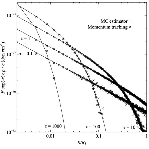
Benchmark for absorption (α = 0). The solid lines indicate the analytical results (Fκρ/c), while values calculated from the MC flux estimator are shown as plusses (+) and those found from following packet momenta are shown as crosses (×). Benchmarks are plotted for spheres of four optical depths (τ = 0.1, 1, 10, 100).
2.1.2 Pure scattering cases
The results of the isotropic, pure scattering benchmark are displayed in Fig. 2. Excellent agreement is seen between the MC estimators and the analytical result, and as expected the noisiest estimator is the momentum tracking algorithm for the τ = 0.1 model.
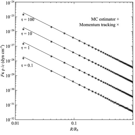
Benchmarks for an isotropic scattering medium (α = 1). Symbols are the same as those for Fig. 1.
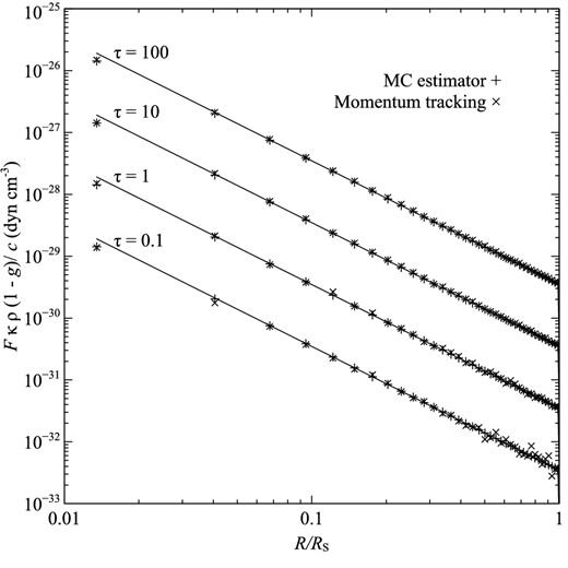
Benchmarks for a scattering medium (α = 1) with a forward-scattering Henyey–Greenstein phase function (g = 0.9). Symbols are the same as those for Fig. 1.
2.2 Radiation pressure hydrodynamic test
Satisfied that the radiation pressure forces were being properly captured by the code, we progressed to testing the treatment in a dynamic model using a similar benchmark to that presented by Nayakshin et al. (2009). A uniform density sphere (ρ0 = 1.67 × 10⁻²² g cc−1 and Rs = 1017 cm) was modelled using 1D grid comprising 1024 uniformly spaced radial cells. The sphere was illuminated by a 1 L⊙ star placed at the centre, and we used 105 photon packets per radiation step.
For the purposes of testing, we assumed isothermal gas at a temperature of 10 K and considered cells above a critical density threshold (1.67 × 10⁻²⁵ g cc−1) to be completely optically thick at all wavelengths with an albedo of zero, while cells with densities below the threshold were considered to be transparent to all radiation. Photon packets entering optically thick cells were immediately absorbed and were not re-emitted, allowing straightforward comparison with analytical results.
We followed the development of the shell for 8 kyr, writing out the radial density profile at 109 s intervals (see Fig. 4), and we then determined the position of the shell for each radial profile. This was done by making a parabolic fit to the peak density in the grid and the density at the adjacent radial grid points. We show the results of the dynamical calculation in Fig. 5. There is good agreement between the model calculation and the theoretical growth of the shell predicted by equation (18). Deviations from theory at late times may be attributed to departures from the thin shell approximation.
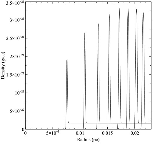
The development of the radiation-pressure-driven spherical shell as a function of time. The mass density as a function of radius is plotted at 1000 kyr intervals from a simulation time of 1000–8000 kyr. Some broadening of the shell is evident at later times.

The evolution of the shell radius with time for the radiation pressure hydrodynamic test (solid line). The theoretical shell expansion based on the thin-shell approximation is also shown (dashed line).
3 PACKET SPLITTING
The splitting of particles in the MC method has a long history, dating back to the first neutron transport codes (Cashwell & Everett 1959). Splitting and its inverse, the so-called Russian Roulette method, are variance reduction techniques designed to improve the efficiency with which the MC sampling operates. Although the original Lucy (1999) algorithm had equal energy photon packets, this is not a fundamental restriction. In the case of star formation calculations, the photon packets may be produced within gas with very high optical depth, and the packets may undergo thousands of scattering events prior to emerging from the computational domain. The MC estimators of the energy density and radiation pressure will be good quality for the optically thick cells where packets spend most of their time, and thus it is inefficient to use equal energy packets. Instead, we employ a packet splitting algorithm, in which a lower number of higher energy packets (Nhigh) are released from the protostar. These propagate through the optically thick region and then are each split into a number of lower energy packets (Nlow) in the optically thin region (see Fig. 6). The total number of packets that emerge from the grid is then N = NhighNlow. The key is to correctly identify the point at which the packet splitting takes place, in order that (i) high-energy packets do not propagate into optically thin regions, since they will increase the noise in the MC estimators, (ii) low-energy packets undergo a small (but non-zero) number of interactions before leaving the computational domain.
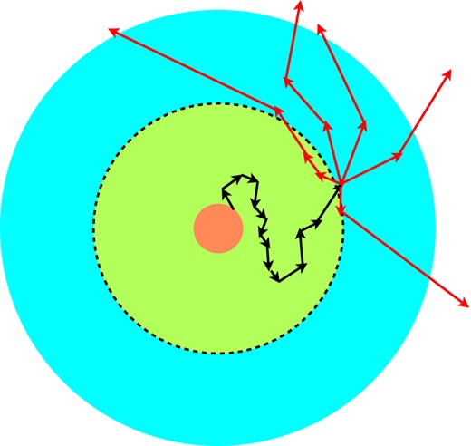
A cartoon illustrating the packet splitting method. A high-energy packet is released from the protostar and undergoes many absorption and scattering events (black arrows). Eventually the packet passes beyond the region identified as being optically thick (dashed line) and at this point the packet is split into Nlow low-energy packets (red arrows) which eventually emerge from the computational domain (here Nlow = 5).
We constructed a one-dimensional test model for the packet splitting algorithm, comprising a 0.1-pc radius sphere containing 100 M⊙ of gas and an r−2 density profile. The dust opacity was from Draine & Lee (1984) silicates with a dust-to-gas density ratio of 1 per cent. The dust is heated by a central luminous protostar of Teff = 4000 K and radius R = 150 R⊙. We first calculated the radiative equilibrium without packet splitting using N = 105 photon packets, and used the final iteration of the radiative equilibrium calculation as our benchmark. We subsequently ran the same model with packet splitting and Nhigh = 1000 and Nlow = 100, defining the high optical depth region as that for which the Planck-mean optical depth to the sphere radius was 20. Note that in two- or three-dimensional problems the integral of the Planck-mean optical depth is calculated in the positive and negative directions of each coordinate axis, defining a typically ellipsoidal boundary for packet splitting.
We plot the temperature profile of the sphere in Fig. 7 for both cases, and find good agreement. In particular there is a smooth change in the temperature through the optical depth boundary (the region where the packet splitting occurs).
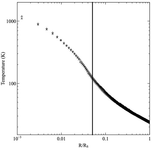
The results of the packet splitting test. The temperature of the sphere is plotted as a function of radial distance (in units of the sphere radius Rs = 0.1 pc). The model without packet splitting (+) shows excellent agreement with the temperature found using packet splitting (×). The vertical line indicates the radius beyond which the high-energy packets undergo splitting.
In the calculation without splitting each photon packet undergoes ∼20 000 absorption or scattering events prior to its emergence from the computational domain. When packet splitting is enabled each high-energy photon packet still undergoes ∼20 000 absorptions or scatterings, but the low-energy photon packets only undergo ∼200. This results in a speed-up of the radiation step of a factor of ∼50.
4 PARALLELIzATION
The primary drawback in such a detailed treatment of the radiation field is the computational effort involved. Fortunately the MC method, in which the photon packets are essentially independent events, may be straightforwardly and effectively parallelized. The top level of parallelization involves domain decomposing the octree that stores the AMR mesh. Each sub-domain belongs to a separate message passing interface (MPI) thread, enabling the code to run on distributed memory machines and enabling the use of domains with a larger memory footprint than that available on a single node. We choose a simple domain decomposition, which although not necessarily load balancing, does allow a straightforward implementation in the code. For eight-way decomposition, each branch of the octree is stored on an individual MPI process (with an additional thread that performs tasks such as passing photon packets to threads). Similarly 64-way decomposition may be achieved by domain decomposing further down the branches of the octree, and this is the decomposition that is employed for majority of our runs (although 512-way decomposition is implemented we do not have access to the resources necessary to regularly run the code in this mode).
The main bottleneck is the communication overhead when passing photon packets between threads, and we optimize this by passing stacks of photon packet data between the MPI threads rather than individual packets in order to reduce latency. Thus, when a photon packet reaches a boundary between domains (naturally this always corresponds to cell boundary) then the packet position, direction, frequency, and energy of the photon packet is stored on a stack. Once the stack reaches a set number of packets (typically 200), then the stack is passed to the appropriate MPI thread. We note that this algorithm closely resembles the MILAGRO algorithm described by Brunner et al. (2006). Further optimization of the stack size is possible, including varying the stack size across the domain boundaries and dynamically altering the stack size as the calculation progresses, but we have yet to implement this.
A further level of parallelization is achieved by having many versions of identical computational domains (which we refer to as hydrodynamic sets), over which the photon packet loop is split, with the results derived from the radiation calculation (radiation momenta, cell integrals etc.) collated and returned to all the sets at the end of each iteration. The thermal balance and ionization equilibrium calculations (which can be time consuming) are then parallelized over the sets, with each thread corresponding to a particular domain performing the equilibrium over an appropriate fraction of its cells before the results are collated and distributed (see Fig. 8).
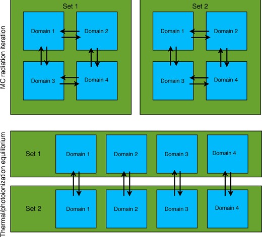
A schematic showing the parallelization of the radiation loop in torus. Here, the photon packets are split across two sets of the AMR mesh (green squares) and each mesh is divided into four domains (blue squares), with inter-domain communication of photon packets (indicated by the black arrows). At the end of the iteration the MC estimators are combined for each domain in order to compute revised temperatures and ionization fractions of the gas.
We performed a scaling test to demonstrate the efficacy of our scheme. We ran the model detailed in Section 3 in 2D. The benchmark used one hydrodynamics set with the quadtree domain-decomposed over four threads, giving a total of five MPI threads including the control thread. We recorded the wall time for one radiative transfer step, and subsequently ran the same model for 3, 6, and 12 hydrodynamics sets (corresponding to 15, 30, and 60 MPI threads, respectively). We found excellent scaling (see Fig. 9) up to 60 threads, with the slight deviation from embarrassing scalability due to the all-to-all MPI communication necessary when the results of the MC estimators are gathered (this is approximately 10 per cent of the wall time for the 60 thread run)
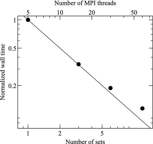
Results of the scaling test of the parallelization. The same 2D model was run with 1, 3, 6, and 12 hydrodynamics sets, corresponding to 5, 15, 30, and 60 MPI threads. The wall time for one radiation timestep is shown (normalized by the five-thread calculation). The solid line indicates perfect scaling.
5 SINK PARTICLE IMPLEMENTATION
We implemented a Lagrangian sink particle scheme within torus in order to follow the formation of stars in our hydrodynamics code. Originally adopted for SPH solvers (Bate, Bonnell & Price 1995), sink particles allow one to overcome the restrictively small Courant time associated with high densities as the collapse proceeds, by removing gas from the computation and adding it to point-like particles that interact with the gas via gravity (and possibly radiation), but not via thermal gas pressure.
The fundamental principles for creating a reasonable sink particle implementation are (i) creating sink particles only as a ‘last resort’, (ii) accreting gas in a manner that has minimal impact on the dynamics of the gas immediately around the sink particle, (iii) properly accounting for the gravitational forces between Lagrangian sink particles and the gas on the grid.
The use of sink particles in grid-based hydrodynamics codes has been investigated by Krumholz, McKee & Klein (2004) and Federrath et al. (2010). Broadly speaking the two implementations described deal with items (i) and (iii) in the same manner, but differ in the way that accretion is treated. The Federrath et al. method defines an accretion radius (as a small multiple of the smallest cell size in their AMR mesh) and simply tests that gas in cells within the accretion radius is bound to the sink particle, and then accretes the gas mass (and its associated linear and angular momentum) above a threshold density on to the sink particle. The Krumholz et al. method uses a dynamically varying accretion radius, which ranges from four-cells to the Bondi–Hoyle radius. The method then ascribes an accretion rate on to the sink based on Bondi–Hoyle–Lyttleton accretion and removes the appropriate mass from each cell within the accretion radius based on a weighting function that falls rapidly with distance from the sink (cells outside the accretion radius have a weighting of zero). The advantage of this method is that an appropriate accretion rate is maintained in situations where the Bondi–Hoyle radius is unresolved, whereas the Federrath method breaks down in this regime. However, the Krumholz method relies on a statistical smoothing of the flow in order to determine the appropriate far-field density and velocity to use when calculating the Bondi–Hoyle accretion rate. In contrast the Federrath method relies primarily on the accretion flow being supersonic outside the accretion radius, and therefore the algorithm by which material is removed from the grid has no impact on the upstream dynamics.
In our implementation, we use a method akin to Federrath's, since we are always in the regime where the Bondi–Hoyle radius is well resolved. Below we describe the details of our sink particle implementation, and several accretion and dynamics tests of the method.
5.1 Sink particle creation
We adopt the same criteria for sink particle creation as Federrath et al. (2010). For the cell under consideration, we define a control volume that contains all cells within a predefined radius racc. Before a sink particle is created a number of checks on the hydrodynamical state of the gas in the control volume must be passed, briefly.
The central cell of the control volume must have the highest level of AMR refinement.
The density of the central cell must exceed a predefined threshold density ρthresh, thus ensuring that |${\nabla } \cdot (\rho {\boldsymbol v}) < 0$| for that cell.
Flows in cells along the principle axes must be directed towards the central cell.
The gravitation potential of the central cell must be the minimum of all the cells in the control volume.
The control volume must be Jeans unstable, i.e. |Egrav| > 2Eth.
The gas must be in a bound state, i.e. Egrav + Eth + Ekin < 0, where Ekin is the kinetic energy of the gas in the control volume where the speeds are measured relative to the velocity of the centre of mass of the control volume.
The control volume must not overlap with the accretion radius of any pre-existing sink particles.
If these tests are passed then a sink particle is created at the centre of the control volume, and accretes gas according to the method detailed below.
5.2 Accretion on to sink particle
5.3 Sink particle motion
For the cell containing the sink particle, we instead perform a sub-grid calculation by splitting the mass of the cell into 83 sub-cells and sum the force over the sub-cells in an analogous manner (equation 20).
The sink–sink interaction is computed using a sum of the gravitational forces over all sinks (this is computationally tractable since the number of sink particles is small). The equation of motion of the sink particles is integrated over a timestep by using the Bulirsch–Stoer method (Press et al. 1993), once again using the cubic spline softening of Price & Monaghan (2007).
5.4 Gas motion
The self-gravity of the gas is solved using a multigrid solution to Poisson's equation, and with the gradient of the potential appearing as a source term in hydrodynamics equations.
6 SINK PARTICLE DYNAMICS TESTS
Following Hubber et al. (2011), we adopt the three-body Pythagorean test problem of Burrau (1913) to benchmark the sink–sink gravitational interactions and test the integrator. This problem has masses (taking G = 1) of m1 = 3, m2 = 4, and m3 = 5 starting at rest at Cartesian coordinates (1, 3), (−2, −1), and (1, −1), respectively. The subsequent motion of the masses involves a number of close interactions between sinks, and was first numerically integrated by Szebehely & Peters (1967). The results of the test problem are given in Fig. 10 and show excellent agreement with figs 2–4 of Szebehely & Peters (1967). The total energy of the system over duration of the computation is conserved to better than 1 part in 106.
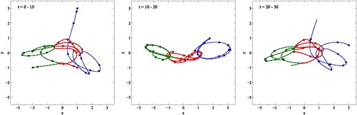
The paths of three masses in the Pythagorean three-body benchmark test. The panels show the paths of the sink particles at t = 0–10 (left-hand panel), t = 10–20 (middle panel), and t = 20–30 (right-hand panel). Mass 1 is shown as a green, dashed line, mass 2 as a red, solid line, and mass 3 as a blue, dotted line. Solid circles indicate the position of the particles at unit time intervals.
The implementation of the gas-on-sink gravitational force calculation was tested by using a power-law (ρ ∝ ρ(r)−2) density sphere of 100 M⊙ and radius 0.1 pc, on a 3D AMR mesh with minimum cell depth 6 (equivalent to a fixed-grid resolution of 64 × 64 × 64) and maximum cell depth 10 (1024 × 1024 × 1024). The computational domain was divided over 64 MPI threads. Three test sink particles of negligible mass were placed in the grid at radii of 2.5 × 10¹⁷, 1 × 10¹⁷, and 5 × 1016 cm, at the appropriate Keplerian orbital speed (∼2.074 km s−1). The hydrodynamics of the gas was neglected for this test, and the sink particles were allowed to move through the stationary gas under gravitational forces only. The benchmark test was run for 130 orbits of the innermost particle (corresponding to ∼26 orbits of the outermost particle). The orbits of the particles are overlaid on the density distribution and adaptive mesh in Fig. 11, indicating that the integrator, domain decomposition, and gas-particle forces are operating satisfactorily.
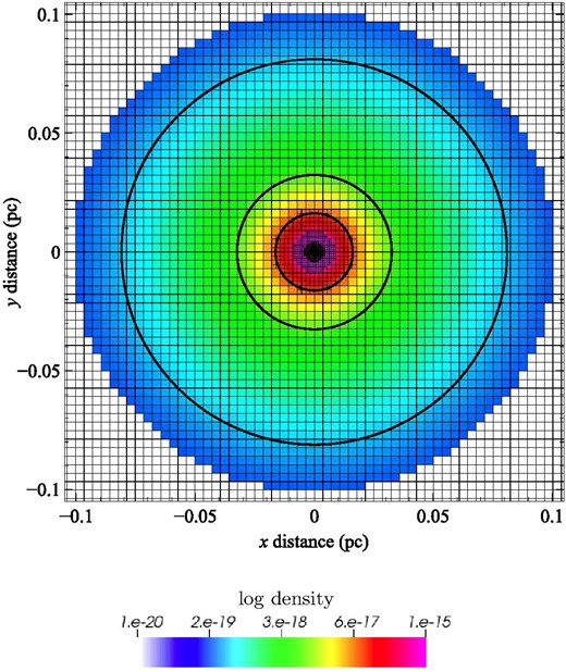
The results of the gas-on-sink gravitational force test. The paths of the three test sink particles are shown as bold solid lines, whilst the density of the gas is shown as a logarithmic colour scale. The AMR mesh is shown by thin solid lines.
7 ACCRETION TESTS
The principle tests of our sink particle implementation are those that ensure that the accretion of gas occurs at the correct rate. We therefore conducted three benchmark tests of increasing complexity.
7.1 Bondi accretion
For this test, we adopted M = 1 M⊙ and ρ∞ = 10−25 g cc−1, giving an expected accretion rate of 5.9 × 10⁻¹¹ M⊙ yr−1and a Bondi radius of 3.75 × 1017 cm. We ran three two-dimensional models with resolutions of RB/Δx of 5, 10, and 20. Rapid convergence in the accretion rate with resolution is observed (see Fig. 12). The highest resolution model has an accretion rate of 5.7 × 10⁻¹¹ M⊙ yr−1, i.e. within 2 per cent of the theoretical rate.
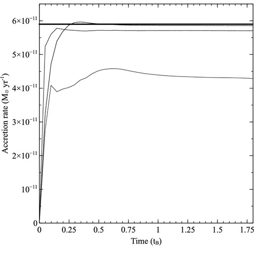
Results of the Bondi accretion test. The accretion rate is plotted against the Bondi time-scale (tB = RB/cs) for the RB/Δx = 5, 10, and 20 models (dotted, dashed, and solid lines, respectively). The thick solid line corresponds to the expected theoretical rate of 5.9 × 10⁻¹¹ M⊙ yr−1.
7.2 Collapse of a singular isothermal sphere
Shu (1977) showed that an isothermal sphere with ρ(r) ∝ 1/r2 collapses in such a way that there is a constant mass flux through spherical shells. The added level of complexity over the Bondi test described above is that the self-gravity of the gas is significant.
We adopt the same test as Federrath et al. (2010), with a sphere of radius R = 5 × 1016 cm with ρ = 3.82 × 10⁻¹⁸ g cm−3 with contains 3.02 M⊙ of gas. The sound speed of the gas was taken to be 0.166 km s−1. The expected accretion rate of this model is 1.5 × 10⁻⁴ M⊙ yr−1. We adopted an adaptive, two-dimensional cylindrical mesh for four levels of refinement, with the smallest cells of R/Δx = 300.
The model demonstrated excellent agreement with the Shu prediction, starting with an accretion rate of ∼1.5 × 10⁻⁴ M⊙ yr−1, and only declining when 90 per cent of the original mass had been accreted (see Fig. 13). At the end of the run the local density approached the global floor density for the simulation (10−21 g cc−1) and the accretion rate approaches the Bondi rate for that density.
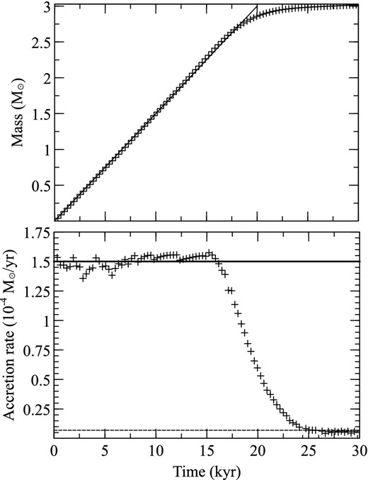
Results of the Shu accretion test. The lower panel shows the accretion rate as a function of time (crosses), with the expected theoretical accretion rates predicted by the Shu model (solid line) and Bondi accretion at the floor density (dashed line). The upper panel shows the growth of the central object as a function of time (crosses) along with the expected trend assuming a constant Shu accretion rate (solid line).
7.3 Bondi–Hoyle accretion
We constructed a 2D test case in which a 1 M⊙ sink is placed at the origin in initially uniform density gas (10−25 g cc−1) with molecular weight of 2.33 and a temperature of 10 K. The gas initially had a constant velocity with a Mach number of |${\cal M}=3$| parallel to the z-axis, and an inflow condition at the upstream boundary and outflow condition at the downstream boundary. These are the same initial conditions as the Bondi–Hoyle test case in Krumholz et al. (2004), although they ran their simulation in 3D.
The model extent was 0.78 pc, and three levels of refinement were used with the smallest cells corresponding to 2.3 × 1014 cm. We ran the model until an approximately steady-state of the accretion rate was achieved (Fig. 14). The theoretical Bondi–Hoyle accretion rate for these conditions is 1.7 × 10⁻¹² M⊙ yr−1, but the Krumholz et al. (2004) model, and those of Ruffert (1996), found accretion rates of close to 2 × 10⁻¹² M⊙ yr−1, with considerable temporal variation in the accretion rate on the Bondi–Hoyle time-scale. Our simulation reached a steady-state accretion rate of 2.4 × 10⁻¹² M⊙ yr−1(Fig. 15), which is comparable to the peak accretion rate seen in the Krumholz et al. (2004) simulations. The level of variability is substantially lower in our simulation, presumably because the instabilities that build up and modify the dynamics near the sink in the 3D simulations are absent in our 2D models.

Bondi–Hoyle accretion test. The figure shows logarithmically scaled density between 10−23 g cc−1 (pink) and 10−25 g cc−1 (black). The white arrows show velocity vectors, with the longest arrows corresponding to speeds of 3 km s−1. The black semicircular region at the origin signifies the extent of the accretion region.
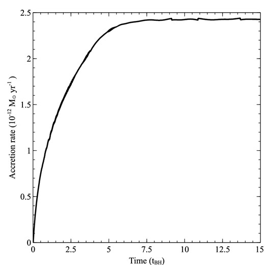
Bondi–Hoyle accretion as a function of time. Time is given in units of the Bondi–Hoyle time-scale, while the accretion rate is given in units of 10−12 M⊙ yr−1.
8 CONCLUSIONS
We have presented a new method for including radiation pressure in RHD simulations that incorporates a level of microphysical detail that is significantly greater than that of FLD or hybrid techniques. We have shown that the new method works in both the pure absorption and pure scattering regimes, and properly treats anisotropic scattering processes. The method comprises a simple addition to the MC estimators required for radiative and photoionization equilibrium calculations, and does not therefore represent a substantial computational overhead to the MC RHD methods described by Haworth & Harries (2012).
However, the MC method as a whole is significantly more computationally demanding than the FLD and hybrid methods, and we have therefore developed two new methods to ameliorate this. The first is the packet splitting method detailed in Section 3, in which we extend Lucy's original algorithm to incorporate photon packets with varying energy. The second is to distribute the MC photon packet loop over many instances of the computational domain, allowing an excellent scalability (see Section 4).
The final element needed to compute massive star formation models is a description of the protostar itself, and to do this we have included a sink particle algorithm. By interpolating on protostellar evolutionary model grids (e.g. Hosokawa & Omukai 2009) as a function of mass and accretion rate will be able to determine temperatures and luminosities for our protostar, and assign it a spectral energy distribution from appropriate atmosphere models. The sink particles then become the origin of photon packets for the RHD calculation.
The next stage is to compute massive star formation models that incorporate radiation pressure and ionization feedback. Initially these models will be two dimensional, but we also conduct three-dimensional calculations in order to simulate binary star formation. Of course the algorithms detailed here have wider applicability, and the correct treatment of feedback from ionization, radiation pressure, and winds is important for cluster-scale calculations, in particular with reference to gas dispersal from clusters (e.g. Rogers & Pittard 2013).
The calculations for this paper were performed on the University of Exeter Supercomputer, a DiRAC Facility jointly funded by STFC, the Large Facilities Capital fund of BIS, and the University of Exeter, and on the Complexity DiRAC Facility jointly funded by STFC and the Large Facilities Capital Fund of BIS. TJH acknowledges funding from Exeter's STFC Consolidated Grant (ST/J001627/1). I am grateful to Jon Bjorkman for useful advice on forward scattering given over cocktails provided by Kenny Wood. Dave Acreman, Tom Haworth, Matthew Bate, and Ant Whitworth are thanked for useful discussions.
