


Abstract
We investigate the correlation between extinction and H i and CO emission at intermediate and high Galactic latitudes (|b| > 10°) within the footprint of the Xuyi Schmidt Telescope Photometric Survey of the Galactic anticentre (XSTPS-GAC) on small and large scales. In Paper I, we present a three-dimensional (3D) dust extinction map within the footprint of XSTPS-GAC, covering a sky area of over 6000 deg2 at a spatial angular resolution of 6 arcmin. In the current work, the map is combined with data from gas tracers, including H i data from the Galactic Arecibo L-band Feed Array H i survey and CO data from the Planck mission, to constrain the values of dust-to-gas ratio DGR = AV/N(H) and CO-to-H2 conversion factor XCO = N(H2)/WCO for the entire GAC footprint excluding the Galactic plane, as well as for selected star-forming regions (such as the Orion, Taurus and Perseus clouds) and a region of diffuse gas in the northern Galactic hemisphere. For the whole GAC footprint, we find DGR = (4.15 ± 0.01) × 10−22 mag cm2 and XCO = (1.72 ± 0.03) × 1020 cm− 2 (K km s− 1)− 1. We have also investigated the distribution of ‘CO-dark’ gas (DG) within the footprint of GAC and found a linear correlation between the DG column density and the V-band extinction: |$N({\rm DG}) \simeq 2.2 \times 10^{21} (A_V - A^{c}_{V})\,\rm cm^{-2}$|. The mass fraction of DG is found to be fDG ∼ 0.55 towards the Galactic anticentre, which is respectively about 23 and 124 per cent of the atomic and CO-traced molecular gas in the same region. This result is consistent with the theoretical work of Papadopoulos et al. but much larger than that expected in the H2 cloud models by Wolfire et al.
1 INTRODUCTION
The interstellar medium (ISM) makes up between 10 and 15 per cent of baryonic mass of the Milky Way. About 99 per cent of the material is in gas form and the rest is in solid dust grains. Observation of the interstellar dust and gas is a primary tool to trace the structure and distribution of molecule clouds, where the star formation takes place. The dominant molecular gas in the ISM is H2, a homonuclear diatomic molecule with no permanent dipole moment and allowed dipole rotational transitions. The most easily excited H2 transition is the quadrupole S(0): Ju → Jl = 2 → 0, which has an excitation energy ΔE20/k ∼ 510 K, more than an order of magnitude higher than the typical kinetic temperature Tkin ∼ 10–50 K of the ISM. As a consequence, H2 is hard to excite and observe, and one has to trace the molecular gas and determine the H2 column density, N(H2), by other indirect methods. Two of the most commonly used tracers are CO gas emission and dust extinction.
Heteronuclear diatomic molecule CO is the most abundant molecule in the ISM after H2. The 12CO J = 1 → 0 transition has a ΔE10/k about 5.5 K and can be easily excited even in cold molecular clouds and observed from the ground. As a consequence, CO has become the primary tracer of the interstellar molecular gas. The molecular abundance ratio CO/H2 is about 10−4. The CO (J = 1→0) survey of Dame, Hartmann & Thaddeus (2001) is the most complete survey which covers the Milky Way of Galactic latitudes |b| ≤ 30°. There are a large number of other CO surveys covering small sky regions around the individual molecular clouds, such as the Orion and the Monoceros clouds (Hartmann, Magnani & Thaddeus 1998; Magnani et al. 2000; Wilson et al. 2005). Planck Collaboration XIII et al. (2014) have extracted the full-sky CO emission in three lines, the J = 1→0, J = 2→1 and J = 3→2 lines at 115, 230, and 345 GHz from the Planck data using a component separation method. The 12CO(J = 1→0) emission at wavelength λ = 2.6 mm is then utilized to determine the total column density of molecular gas assuming a CO-to-H2 conversion factor, the so-called X factor, which relates the surface brightness of CO emission and the column density of molecular gas, XCO = N(H2)/WCO (cf. Bolatto, Wolfire & Leroy 2013 for a review), where WCO is the velocity-integrated brightness temperature of 12CO J = 1 → 0. The XCO factor works best for cloud ensemble averages. The minimum averaging scale would be that of a single Giant Molecular Cloud (GMC), ∼10–100 pc (Dickman, Snell & Schloerb 1986; Young & Scoville 1991; Bryant & Scoville 1996; Regan 2000; Papadopoulos, Thi & Viti 2002). The most quoted value of X factor for the Milky Way is XCO ∼ 2 × 1020cm− 2 (K km s− 1)− 1 (Frerking, Langer & Wilson 1982; Dame et al. 2001; Lombardi, Alves & Lada 2006).
The visual interstellar extinction AV has been found to have a linear relationship with the total column density of hydrogen nuclei N(H). The relationship is a cornerstone of the modern astrophysics. The classic value of the constant of proportionality, i.e. the dust-to-gas ratio, DGR = AV/N(H), derived from the measurements of the ultraviolet (UV) absorption of the H i Lyα line and the H2 Lyman band towards a small number of early-type stars with the Copernicus satellite (Savage et al. 1977; Bohlin, Savage & Drake 1978), is DGR = 5.34 × 10− 22 mag cm2. More recently, Liszt (2014a,b) trace |$N(\rm {\rm H\,\small {i}})$| and E(B − V) across the sky of Galactic latitudes |b| = 20–60°. They consider data only of relatively low extinction, 0.015 < E(B − V) < 0.075 mag, for which the hydrogen should mostly be in the form of neutral atoms and thus the corrections of |$N(\rm {\rm H\,\small {i}})$| for saturation and H2 formation are unlikely important. From the data, they obtain a DGR value (3.73 × 10− 22 mag cm2) that is smaller compared to the reference value. The column density of atomic hydrogen, |$N(\rm {\rm H\,\small {i}})$|, can be determined by measuring the H i 21 cm emission. Thus, if one can accurately determine the extinction and value of DGR, then the H2 column density can be derived using the relation |$N({\rm H_2})=A_V/DGR-N(\rm {\rm H\,\small {i}})$|. There are several successful large H i 21 cm emission surveys of the Galaxy, including the Leiden–Argentine–Bonn (LAB) full-sky survey (Kalberla et al. 2005), the international Galactic Plane Survey (IGPS; Taylor et al. 2003), the Galactic All Sky Survey (GASS; McClure-Griffiths et al. 2005) in the Southern hemisphere, and the Galactic Arecibo L-band Feed Array H i survey (GALFA-HI; Peek et al. 2011) targeting both the Galactic plane and high latitude regions.
Dust grains can be traced by extinction in the visible and in the near-infrared (IR). Chen et al. (2014, hereafter Paper I) estimate values of extinction and distance to over 13 million stars catalogued by the Xuyi 1.04/1.20 m Schmidt Telescope photometric survey of the Galactic anticentre (XSTPS-GAC; Zhang et al. 2013, 2014; Liu et al. 2014). They derive the extinction by fitting the spectral energy distribution (SED) for a sample of 30 million stars that have supplementary IR photometry from the Two Micron All Sky Survey (2MASS; Skrutskie et al. 1997) and the Wide-Field Infrared Survey Explorer (WISE; Wright et al. 2010). Together with the photometric distances deduced from the dereddened XSTPS-GAC optical photometry, Paper I construct a 3D r-band extinction map within the GAC footprint at a spatial resolution, depending on the latitude, that varies between 3 and 9 arcmin. The 3D map of Paper I has also been used to construct a 2D extinction map, integrated to a distance of 4 kpc, approximately the maximum distance that dwarf stars in the sample can trace with sufficiently high photometric accuracy. The dust extinction within this distance is well constrained. The map has an angular resolution of 6 arcmin and is also publicly available.1 In the current work, this 2D extinction map is used to investigate the dust-to-gas ratio and the X factor within the footprint of XSTPS-GAC.
There are a number of well-known large star-forming regions within the footprint of XSTPS-GAC, such as the Perseus, Taurus and Orion clouds. They form parts of the Gould Belt. Those clouds are in the southern Galactic plane, located at relatively small distances (d < 800 pc; Paper I). We study the correlation between the interstellar dust and gas for these regions. Within these regions there exist diffuse, non-self-gravitating clouds as well as dense, massive, self-gravitating, star-forming clouds like the Orion. Several studies on the dust and gas correlation have been carried out for those individual clouds. Pineda, Caselli & Goodman (2008a), Goldsmith et al. (2008) and Pineda et al. (2010) study the Taurus molecular cloud, while Pineda et al. (2008b) and Lee et al. (2012, 2014) focus on the Perseus cloud and Digel et al. (1999), Ackermann et al. (2012) and Ripple et al. (2013) on the Orion cloud.
One can measure the amount and distribution of the atomic and molecular gas as well as the dust grains by combining various tracers. In this paper, we combine the dust extinction together with gas distribution traced by H i data from the GALFA-HI (Peek et al. 2011) and CO data from the Planck mission (Planck Collaboration XIII et al. 2014), to constrain the values of DGR and XCO at a high angular resolution of 6 arcmin. The existence of molecular gas of low CO abundance has been noted previously in theoretical models (van Dishoeck & Black 1988; Papadopoulos et al. 2002), in observations of diffuse gas and high-latitude clouds (Lada & Blitz 1988) and in observations of irregular galaxies (Madden et al. 1997). The values of DGR and XCO determined in the current work allow us to further trace this so-called ‘CO-dark gas’ (DG; Reach, Koo & Heiles 1994; Meyerdierks & Heithausen 1996; Grenier, Casandjian & Terrier 2005; Abdo et al. 2010) at both small and large scales. We are not the first one on this topic of course. For example, Planck Collaboration XIX et al. (2011) has obtained an all-sky map of dust optical depth and compared it with the observed distribution of gas column density. The results are used to constrain the correlation between the dust and gas, (τD/NH)ref, as well as the values of XCO, and to construct a distribution map of DG at high and intermediate Galactic latitudes (|b| > 10°). Paradis et al. (2012) carry out a similar study using the extinction data deduced from the colour excess of the 2MASS photometry instead of those derived from the far-IR optical depth. Both the work of Paradis et al. (2012) and Planck Collaboration XIX et al. (2011) are limited by the angular resolution of the LAB 21 cm H i emission survey (Kalberla et al. 2005), which is 36 arcmin. In the current work we have adopted data from the GALFA-HI survey. As a consequence, the angular resolution has been improved significantly.
The paper is structured as the following. In Section 2 we present the 2D extinction map integrated to a distance of 4 kpc. Section 3 describes the data of gas tracers used in the current analysis. The correlations between extinction and gas content are investigated in Section 4 with the main results discussed in Section 5. We summarize in Section 6.
2 THE EXTINCTION MAP
The photometric extinction and distance catalogue of Paper I is first used to construct a 2D extinction map integrated to a distance of 4 kpc for the footprint of XSTPS-GAC. The catalogue contains more than 13 million stars with estimates of r-band extinction and photometric distance. To ensure good photometric accuracy, only objects flagged with a quality flag ‘A’, i.e. with average photometric errors less than 0.05 mag for all the eight bands used to derive the extinction and distance (g, r, and i from the XSTPS-GAC, J, H and KS from the 2MASS, and W1 and W2 from the WISE), are included (Sample A of Paper I). Possible candidates of giants, flagged as ‘G’, are excluded because their distances may have been grossly underestimated. This leaves just over 7 million stars and they are divided into sub-fields of size 6 × 6 arcmin2. For each sub-field, a sliding window of depth 450 pc, stepping by steps of 150 pc, is used to obtain the median value of extinction for each distance bin. The extinction as a function of distance, |$A_r^i(d)=f_i(d)$|, where i is the index of sub-fields, is then obtained after applying a boxcar smoothing of width 450 pc. The extinction versus distance relations of all sub-fields (sightlines) are used to construct a 3D extinction map, which is then integrated out to a distance of d = 4 kpc to yield a 2D extinction map to be used in the current analysis. Most of the sample stars are within a distance of 4 kpc and the extinction out to this distance is well constrained. The 4 kpc integrated map can be treated as a lower limit of extinction map along the sightlines.
Fig. 1 presents the 4 kpc dust extinction map thus derived. It has a spatial resolution of 6 arcmin. The resolution is chosen to ensure that most of the subfields have a sufficient number of stars (>10) to derive a robust relation of extinction as a function of distance. For a small fraction of sub-fields (less than 1.5 per cent) of high Galactic latitudes or suffering from high extinction, there are not enough numbers of stars of high photometry accuracies available. For those fields, we have adopted some stars of lower accuracy from the catalogue (Sample C of Paper I). Those sub-fields are flagged by ‘C’. The V-band extinction AV is converted from Ar using the extinction law of Yuan, Liu & Xiang (2013), AV = 1.172Ar, assuming a total-to-selective extinction ratio RV = 3.1. The uncertainties of the map are estimated from the stars located within the distance bin of width 450 pc centred at 4 kpc and in a width of 450 pc. The typical uncertainties are 0.18 mag in AV, or about 0.06 mag in E(B − V). The uncertainties are mainly determined by the stellar density and depth of the sample. Under favourable conditions, the uncertainties could be as low as 0.04 mag in AV. Some ‘stripe-like’ artefacts can be seen on the map. They are caused by the nightly varying survey depth and photometric accuracy of the XSTPS-GAC. A notable empty patch around l ∼ 160° and b ∼ 20° is due to the abnormally large photometric errors of XSTPS-GAC in that area.
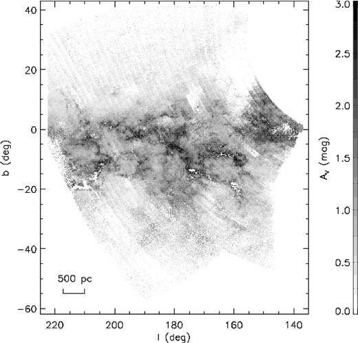
A 2D extinction map, integrated to a distance of 4 kpc for the footprint of XSTPS-GAC. The map has an angular resolution of 6 arcmin.
Paper I have compared their Sample A median extinction map with those of Schlegel, Finkbeiner & Davis (1998) and Froebrich et al. (2007), and found some systematic offsets amongst them. Parts of the differences are clearly caused by the difference in distance traced by the three maps [2–3 kpc for Sample A median extinction map of Chen et al., essentially infinite for the SFD map and about 1 kpc for that of Froebrich et al. (2007), respectively]. The 4 kpc extinction map presented here should have included almost all the dust extinction alone the sightlines for sub-fields of intermediate and high Galactic latitudes (|b| > 10°), thus should be directly comparable with that of SFD. In addition, it should also be comparable with the 4.5 kpc reddening map newly derived from the PanSTARRS (Kaiser et al. 2010) photometry by Schlafly et al. (2014). Fig. 2 compares values of extinction from our 4 kpc extinction map with those of SFD and Schlafly et al. (2014) for sightlines of Galactic latitude |b| > 10°. Values of AV are converted to E(B − V) assuming RV = 3.1. Except for some outliers, our values agrees well with both those of SFD and Schlafly et al. (2014) for E(B − V) < 0.8 mag. In deriving the extinction, both our analyses and those of Schlafly et al. (2014) have made the assumption that all reddening values should be no less than zero. The assumption could introduce some biases, in particular for sightlines of very low, close to zero, extinction. In principle, both the best SED fit algorithm of Paper I and the Bayesian approach of Green et al. (2014) could lead to systematically over-estimated values of extinction for regions of low extinction (Berry et al. 2012; Paper I; Green et al. 2014; Schlafly et al. 2014). Photometric errors obviously contribute to the uncertainties. Other potential sources of error include the colour-reddening degeneracy. Those systematics might be the cause of the significant non-Gaussianity seen in the distribution of differences of values as given by our map and those of SFD (Fig. 2). By contrast, the distribution of differences of values between ours and those of Schlafly et al. (2014) follows closely a Gaussian one, reflecting the fact that both use a similar method to estimate the extinction.
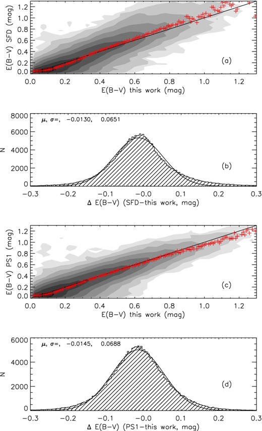
Comparisons of extinction values as given by our map and those given by the SFD map (top two panels), and by the map of Schlafly et al. (2014; lower two panels). The red pluses in the first and third panels represent median values in the individual bins. A black straight line denoting complete equality is also overplotted to guide the eyes. In the second and fourth panels, the black curve is a Gaussian fit to the distribution of differences of values.
For high extinction regions [E(B − V) > 0.8 mag], SFD reddening values are systematically higher than ours while those of Schlafly et al. (2014) map are lower. Most of those highly reddened regions for which our estimates of reddening are significantly smaller than given by the SFD map are actually from low Galactic latitudes. In fact, if we restrict the plots of Fig. 2 to absolute latitudes higher than 20° (|b| > 20°), then the systematic differences between ours and the SFD values disappear. Thus it is very likely, for those highly reddened, low-latitude regions, the integration distance of 4 kpc used to derive our current 2D extinction map is not deep enough. The systematic lower values given by the map of Schlafly et al. (2014) compared to ours for those highly extincted regions are much more difficult to understand, as both analyses use similar methods, although the results are based on different data set. The integration of the Schlafly et al. map is 500 pc further than ours. But instead of giving higher values, the map of Schlafly et al. actually yields lower values compared to ours. Schlafly et al. (2014) notice that when their map is compared to that of SFD, their map yields systematic lower values even for regions of latitudes |b| > 30°. It is possible that Schlafly et al. (2014) may have systematically underestimated the reddening values for some of the highly extincted regions. For the whole XSTPS-GAC footprint of |b| > 10°, our map gives on average only marginally larger values compared to those of SFD and Schlafly et al. (2014), by 0.013 and 0.015 mag, respectively. The scatters of differences between the values are about 0.06 mag in E(B − V), comparable to the typical uncertainties estimated for our map (0.18 mag in AV).
3 GAS TRACERS
The interstellar gas can either be atomic, molecular or ionized. Those three phases are commonly traced by the H i 21 cm emission, by the molecular CO pure rotational transitions and by the H i Hα recombination line, respectively. The ionized gas can also be traced by the free–free emission of thermal electrons. The contribution of the ionized gas, which are mostly restricted to the individual, isolated H ii regions, to the total gas content is neglected in the current study. Only most recently published data that have the highest angular resolutions and best signal-to-noise ratios (SNRs) are employed in this work.
3.1 H i data
We use the H i data from the GALFA-HI survey to trace the content of atomic gas. The GALFA-HI survey uses Arecibo L-band Feed Array, a seven-beam array of receivers mounted at the focal plane of the 305 m Arecibo telescope, to map the H i 21 cm emission in the Galaxy (Peek et al. 2011). The survey aims to cover both the Galactic plane and the high Galactic latitudes with an angular resolution of 3.4 arcmin. The GALFA-HI first data release (DR1) has been presented by Peek et al. (2011). The DR1 data cover 7520 deg2 of the sky, produced from 3046 h worth of data obtained for 12 individual projects. The local standard of rest (LSR) velocity of the emission ranges from −700 to +700 km s− 1. The rms noise in a 1 km s− 1 channel ranges from 140 to 60 mK, with a median of 80 mK. The DR1 data can be downloaded from https://purcell.ssl.berkeley.edu/.
The GALFA-HI DR1 data do not cover the entire footprint of XSTPS-GAC, but only the region of 3h < RA < 9h and 0 < Dec. < 39 deg. This unfortunately restricts the sky coverage of the current work. We use the data of velocity resolution 0.8 km s− 1. The H i column density |$N({\rm {\rm H\,\small {i}}})$| is derived from the profile of brightness temperature after applying a small correction for the optical depth effects assuming a spin temperature of 145 K, as adopted by Liszt (2014a,b). The temperature corresponds to the mean ratio of H i 21 cm emission and absorption (Liszt, Pety & Lucas 2010) measured by the Millennium H i Emission-Absorption Survey of Heiles & Troland (2003). Values of |$N(\rm {\rm H\,\small {i}})$| derived for the XSTPS-GAC footprint range from 1.5 × 10²⁰ to 1.2 × 1022 cm− 2, with a median of 1.4 × 1021 cm− 2. The distribution of |$N(\rm {\rm H\,\small {i}})$| thus deduced is shown in the left panel of Fig. 3.
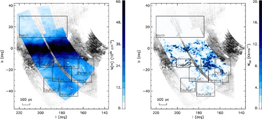
Contours of |$N{\rm ({\rm H\,\small {i}})}$| (left panel) and WCO (right panel) in the footprint of XSTPS-GAC. The grey-scale background image illustrates the 4 kpc extinction map. The squares denote different regions analysed in the current work. The maps have an angular resolution of 6 arcmin.
3.2 CO data
We use the CO-integrated intensity image produced by Planck Collaboration XIII et al. (2014), which is based on the Planck first 15.5 month survey data (two full-sky scans) and uses the full-sky maps of the nine Planck frequency bands, and also the 100, 217 and 353 GHz full-sky bolometer maps. Planck Collaboration XIII et al. (2014) provide all sky maps of the velocity-integrated emission of the CO J = 1 → 0, J = 2 → 1 and J = 3 → 2 transitions. They produce three types of maps. We choose the Type 3 map generated from the multi-line approach. The approach assumes fixed CO line ratios in order to achieve the highest possible SNR, and has an angular resolution of ∼ 5.5 arcmin. The standard deviation of the Type 3 CO(1→0) map, when used at an angular resolution of 15 arcmin, is typically 0.16 K, compared to 1.77 and 0.45 K for the Type 1 and 2 maps, respectively. For comparison, the CO survey of Dame (2011) has a typical uncertainty of 0.6 K. We choose the Planck Type 3 CO (1→0) map because of its high angular resolution and high SNR. Type 3 map is also more suitable for intermediate and high Galactic latitudes (cf. Planck Collaboration XIII et al. 2014 for more detail). There is some 13CO contamination in the Planck CO(1→0) map. To correct for this, we have divided the data by a factor of 1.16 (Planck Collaboration XIII et al. 2014).
Dame et al. (2001) combine data of CO surveys of the Galactic plane and local molecular clouds and produce a composite map of an angular resolution of 8.4 arcmin. The data were obtained with the 1.2 m telescope of the Harvard–Smithsonian Center for Astrophysics. The data published by Dame et al. (2001) are mainly for the Galactic plane. Data of high Galactic latitudes (|b| > 20°) are not available. In this paper, the data of Dame et al. (2001) are only used as a reference to check the data we actually use.
The Planck Type 3 CO-integrated intensity image is presented in the right panel of Fig. 3. We only show the footprint where data of AV, N(H i) and WCO are all available. It shows excellent agreement with the dust extinction map. In this paper, we first bring all input data sets to a common angular resolution determined by the lowest angular resolution data set, which is 6 arcmin of the extinction map. This is done by performing a Gaussian kernel smooth. Thanks to the high resolution, we can analyse the correlation between dust and gas at intermediate Galactic latitudes of the GAC for the individual molecular clouds, such as the Orion, Taurus and Perseus cloud. We divide the clouds into eight different regions. Their positions and ranges on the sky are marked by the squares in Fig. 3, together with a region of diffuse gas without any obvious molecular clouds in the northern Galactic hemisphere, noted as ‘North’ in the current work.
4 EXTINCTION AND GAS CORRELATION
We first assume that there is no DG in all subfields (pixels). We then select pixels where the CO emission is low (WCO < 0.2 K km s− 1). The column density of molecules of those pixels N(H2) must be less than 2.0 × 1019 cm− 2 if one assumes that XCO = 1 × 1020 cm− 2 (K km s− 1)− 1. Given that the minimum column density of atomic gas within the XSTPS-GAC footprint is 1.5 × 1020 cm− 2 (see Section 3.1), the gas column density of those pixels can be considered as being contributed by atomic gas only [N(H)=N(H i)]. Under such assumptions, we then derive the best-fitting values of DGR and |$A^0_V$| of those pixels.
The best-fitting values of DGR and |$A^0_V$| obtained from the last step are then applied to all pixels, and this time the value of XCO is fitted as a free parameter. We have smoothed the data to an angular resolution of 2°, corresponding to about 140 pc at a distance of 4 kpc and 15 pc at a distance of 400 pc (where most of the molecular clouds analysed in the current work, the Orion, Taurus and Perseus clouds locate within) in this step to obtain the statistical cloud-ensemble-average values of XCO (Dickman et al. 1986; Young & Scoville 1991; Bryant & Scoville 1996; Papadopoulos et al. 2002).
The above-derived values of DGR, |$A^0_V$| and XCO are applied to equation (1) to calculate values of |$A^{\rm mod}_V$| of all pixels. A χ2 value is then calculated as |$\chi ^2=\sum _{i} {(A_{V,i} - A^{\rm mod}_{V,i}})$|, where i is the pixel index.
- The column density of DG is then calculated from formula(2)\begin{equation} N({\rm DG})=(A_V-A^{\rm mod}_V)/DGR. \end{equation}
We then go back to the first step, but this time use the DG distribution derived from the previous step. We select pixels that both have low CO emission (WCO < 0.2 K km s− 1) and no DG content [N(DG) ≤ 0 cm− 2]. The fields are used to update the best-fitting values of DGR and |$A^0_V$| and the process is iterated until a minimum χ2 value is reached.
In the current work, we have omitted the Galactic plane which shows very strong atomic gas emission and where the contribution of ionized gas cannot be ignored. Thus only data from Galactic latitudes |b| > 10° are used throughout the paper. Since we have excluded the Galactic-plane clouds, those included are representative of the diffuse cloud component of the Galaxy. Usually a minimum χ2 is reached after the first iteration that assumes there is no DG component at all pixels. We list the results in Table 1 for both the whole XSTPS-GAC footprint of |b| > 10° and for the individual selected regions. Errors of the resultant parameters are derived using a bootstrap method. For each parameter, we apply the algorithm to 1000 randomly selected samples and derive the parameters of those samples. The resultant parameters follow a Gaussian distribution. The variance of the Gaussian distribution is taken as the error of the corresponding parameter.
Dust-to-gas ratio DGR and CO-to-H2 conversion factor XCO derived for individual regions towards the Galactic anticentre.
| Region | DGR | |$A^0_V$| | XCO | |$\frac{M_{\rm H}({\rm DG})}{M_{\rm H}({\rm H\,{\small I}})}$| | |$\frac{M_{\rm H}({\rm DG})}{M_{\rm H}({\rm H^{\rm CO}_2})}$| | fDG | |$\frac{N(\rm DG)}{(A_V-A^c_V)}$| | |$A^c_V$| |
|---|---|---|---|---|---|---|---|---|
| (10− 22 mag cm2) | (mag) | (1020 cm− 2 (K km s− 1)− 1) | 1021 cm−2 mag−1 | (mag) | ||||
| All of |b| > 10° | 4.15 ± 0.01 | 0.06 ± 0.002 | 1.72 ± 0.01 | 0.23 | 1.24 | 0.55 | ||
| Orion 1 | 7.74 ± 0.21 | −0.75 ± 0.05 | 1.54 ± 0.01 | 0.09 | 0.45 | 0.31 | 2.15 ± 0.07 | 1.10 ± 0.05 |
| Orion 2 | 5.53 ± 0.08 | −0.29 ± 0.02 | 1.34 ± 0.03 | 0.10 | 1.43 | 0.59 | 1.69 ± 0.07 | 0.97 ± 0.06 |
| Taurus | 3.65 ± 0.10 | 0.34 ± 0.02 | 1.38 ± 0.01 | 0.22 | 0.31 | 0.24 | 2.75 ± 0.12 | 0.91 ± 0.04 |
| Taurus E1 | 6.42 ± 0.10 | −0.15 ± 0.02 | 0.84 ± 0.01 | 0.11 | 1.43 | 0.59 | 2.28 ± 0.02 | 0.76 ± 0.04 |
| Taurus E2 | 5.62 ± 0.08 | −0.14 ± 0.01 | 1.69 ± 0.04 | 0.11 | 4.01 | 0.80 | 1.89 ± 0.07 | 0.64 ± 0.05 |
| Taurus E3 | 6.33 ± 0.15 | −0.13 ± 0.02 | 1.41 ± 0.02 | 0.13 | 3.42 | 0.77 | 2.28 ± 0.03 | 0.57 ± 0.04 |
| Perseus 1 | 5.01 ± 0.08 | 0.10 ± 0.01 | 1.04 ± 0.01 | 0.18 | 0.89 | 0.47 | 2.10 ± 0.04 | 0.59 ± 0.05 |
| Perseus 2 | 3.24 ± 0.28 | 0.22 ± 0.03 | 2.39 ± 0.01 | 0.22 | 1.05 | 0.52 | 2.36 ± 0.04 | 0.55 ± 0.04 |
| North | 1.38 ± 0.02 | 0.20 ± 0.002 | 0.95 | 2.40 ± 0.03 | 0.22 ± 0.04 |
We present in Fig. 4 the correlation between visual extinction AV and total column density of hydrogen, |$N({\rm H})=N({{\rm H\,\small {i}}})+2X_{\rm CO}W_{\rm CO}$|, for all XSTPS-GAC pixels of |b| > 10°, excluding the Galactic plane. Despite the large scatters, in particular for pixels of low extinction, the data exhibit a significant linear correlation between the two quantities. The data yield a best-fitting value of DGR of (4.15 ± 0.01) × 10− 22 mag cm2. The best-fitting value of XCO is found to be (1.72 ± 0.01) × 1020 cm− 2 (K km s− 1)− 1.
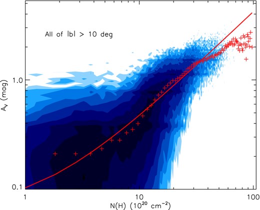
Correlation between the visual extinction AV and the total column density of hydrogen, |$N({\rm H})=N({\rm H\,\small {i}})+2N(\rm H_2)$|, for the whole XSTPS-GAC footprint of |b| > 10° that excludes the Galactic plane. The blue contours represent the density of pixels on a logarithmic scale. The red pluses are median values for the individual N(H) bins. The red solid line is a fit to all the data points.
The southern Galactic hemisphere covered by the XSTPS-GAC survey (b < −10°) includes several prominent GMCs, including the Orion, Perseus, Taurus clouds and the Taurus cloud extension regions. We have earmarked eight regions and examine the gas and dust correlation. We have also applied our algorithm to a region of diffuse gas in the northern Galactic hemisphere, earmarked as ‘North’. The ranges, mean extinction, mean |$N{\rm ({\rm H\,\small {i}})}$| and mean WCO of these regions are listed in Table 2. The positions of those regions are marked by squares in Fig. 3. The CO and extinction maps show remarkably similar features, although those features are not so obvious in the H i map. For those individual regions, the resultant parameters are also listed in Table 1 and the relevant data showing the correlation between AV and N(H) are presented in Fig. 5. Clearly, different clouds seem to have different dust and gas properties. The values of DGR deduced for the individual regions of molecular clouds range from 3.24 × 10⁻²² to 7.74 × 10⁻²² mag cm2. For the diffuse gas region ‘North’, the value is 1.38 × 10⁻²² mag cm2. The values of XCO for different clouds range from 0.84 × 10²⁰ to 2.39 × 1020 cm− 2 (K km s− 1)− 1. The correlation between AV and N(H) is quite good for the individual clouds. In the ‘North’ region, the lack of high CO content pixels makes it very difficult to fit XCO. The dust extinction in this region is also low (most of the pixels have AV < 1 mag), leading to a value of DGR, much smaller than those found for the regions of molecular clouds.
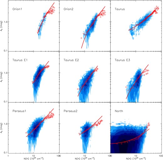
Same as Fig. 4 but for the individual regions. The name of the region is marked in each panel.
Individual regions studied in the current work.
| Region | Longitude | Latitude | |$\overline{A_V}$| (mag) | |$\overline{N({\rm H\,\small {i}})}$| (1020 cm− 2) | |$\overline{W_{\rm CO}}$| (K km s− 1) |
|---|---|---|---|---|---|
| Orion 1 | 211°< l < 201° | −17° < b < −10° | 1.44 | 23.93 | 1.61 |
| Orion 2 | 201°< l < 188° | −18° < b < −10° | 1.04 | 22.31 | 0.56 |
| Taurus | 178°< l < 164° | −19° < b < −10° | 1.38 | 16.47 | 4.22 |
| Taurus E1 | 189°< l < 171° | −31° < b < −17° | 1.02 | 16.78 | 0.75 |
| Taurus E2 | 182°< l < 165° | −45° < b < −32° | 0.70 | 14.62 | 0.12 |
| Taurus E3 | 197°< l < 183° | −41° < b < −28° | 0.66 | 11.96 | 0.16 |
| Perseus 1 | 165°< l < 150° | −25° < b < −10° | 0.93 | 13.35 | 1.30 |
| Perseus 2 | 171°< l < 152° | −32° < b < −25° | 0.65 | 11.49 | 0.49 |
| North | 220°< l < 175° | 10°< b < 30° | 0.31 | 7.70 | 0.00 |
5 DISCUSSION
5.1 Comparison with previous work
The average value of DGR deduced here for the XSTPS-GAC footprint that excludes the Galactic plane, (4.15 ± 0.01) × 10−22 mag cm2, is in good agreement with the results of previous work. It is slightly smaller than the most cited value, 5.3 × 10− 22 mag cm2, derived by Bohlin et al. (1978) from the UV and optical absorption line measurements towards hot stars. It is also slightly smaller than values of (6.0–6.5) × 10− 22 mag cm2 derived from the reddening and the Lyα absorption towards early-type stars (Shull & van Steenberg 1985; Diplas & Savage 1994). On the other hand, Liszt (2014a) finds an even smaller value of 3.7 × 10− 22 mag cm2 from the SFD map combined with 21 cm H i measurements. The values of DGR for the individual cloud regions vary by a factor of 2, from 3.2 to 7.7 × 10− 22 mag cm2. They are also consistent with values from the previous work. Paradis et al. (2012) obtain an average value of 5.46 × 10− 22 mag cm2 for the whole region of the outer Galaxy (|l| > 70°) and values of (3.4–8.7) × 10− 22 mag cm2 for individual regions, in good agreement with our results. A variety of factors may lead to variations of dust-to-gas ratios amongst different regions, including differences in dust content and metal abundance. The dust extinction law of different regions may also differ. Froebrich et al. (2007) discuss variations of the extinction law amongst individual clouds in the GAC area. In fact, we notice that the value of DGR decreases with increasing power-law index β of extinction law in the near-IR. The index β is known to correlate with the dust properties, including the grain size distribution (Draine 2003).
The value of CO to H2 conversion factor, XCO, determined hitherto differs from one analysis to another. Our best-fitting value of 1.72 × 1020 cm− 2 (K km s− 1)− 1 for the whole XSTPS-GAC footprint of |b| > 10° is close to the Galactic average value (Strong & Mattox 1996). The value is slightly lower but nevertheless quite close to the value of (1.8 ± 0.03) × 1020 cm− 2 (K km s− 1)− 1, derived for Galactic regions of |b| > 5° by Dame et al. (2001) based on extinction data from SFD, H i data from the Dwingeloo–Leiden H i survey and CO data from Dame et al. (2001). Glover & Mac Low (2011) demonstrate by numerical simulations that XCO falls off with extinction as |$X_{\rm CO} \propto A^{-3.5}_V$| for clouds of mean extinction smaller than 3 mag. However, our current results do not show that kind of relation. In addition, our derived values of XCO are significantly smaller than predicted by the numerical simulations of Glover & Mac Low (2011). Polk et al. (1988) consider a simple two-component cloud model which consists of GMC cores and lower column density (‘diffuse’) molecular gas. The conversion ratios for the dense cloud cores and the diffuse clouds are different, estimated at ∼4 × 10²⁰ and 0.5 × 1020 cm− 2 (K km s− 1)− 1, respectively. Thus the measured values of XCO in the current work [around ∼ 1.5 × 1020 cm− 2 (K km s− 1)− 1] are closer to those of the diffuse clouds of the work by Polk et al. (1988) than the dense ones, indicating that the clouds in our sample are dominated by the diffuse phases. Pineda et al. (2008a) find that XCO varies from 0.9 to 3.0 × 1020 cm− 2 (K km s− 1)− 1 amongst several regions of the Perseus cloud. Ackermann et al. (2012) find that for the Orion cloud, XCO ∼ (1.3 ∼ 2.3) × 1020 cm− 2 (K km s− 1)− 1. Finally, Abdo et al. (2010) report a significant variations ranging from ∼0.9× to ∼ 1.9 × 1020 cm− 2 (K km s− 1)− 1, from the Gould Belt to the Perseus arm. All those findings are all in good agreement with our results.
5.2 Validation of the gas tracers
Both Planck Collaboration XIX et al. (2011) and Paradis et al. (2012) assume that the 21 cm line is optical thin when calculating the column density of atomic gas. Fukui et al. (2015) infer that the DG in the Galaxy is dominated by optically thick and cool H i gas, which implies that the average density of H i is two times higher than that derived assuming optically thin in the local interstellar space. In this work we have applied a first-order opacity correction, assuming a constant Ts for the emission. The need to correct for the opacity effects in the 21 cm line profiles ultimately limits the accuracy of N(H) determinations. We find that for most directions towards the GAC but out of the Galactic plane, the column densities of neutral hydrogen derived are systematically higher than those deduced assuming optically thin. A comparison of H i column densities derived assuming optically thin and those assuming a constant Ts = 145 K is presented in the left panel of Fig. 6. The latter values are 1.1–1.3 times higher than their optically thin counterpart.
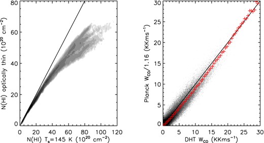
Left panel: comparison of atomic hydrogen column densities derived assuming a constant spin temperature of Ts = 145 K and those deduced assuming optically thin emission. Right panel: comparison of the corrected Planck CO data and those of Dame et al. (2001). The red pluses are median values for the individual bins and the black solid lines represent the line of equal.
In the right panel of Fig. 6, we compare the Planck CO data with those of Dame et al. (2001). The Planck Type 3 CO data are in good agreement with those of Dame et al. (2001), after correcting for a constant slope of 1.16. We have investigated the parameters for the overlapping subfields using the CO data of Dame et al. (2001) instead of those of Planck. It yields consistent results very similar to those presented here.
5.3 The CO-dark gas
There is a clear excess of AV as given by the extinction map compared to the simulated |$A^{\rm mod}_V$| for regions of N(H) > 1.2 × 1021 cm− 2 (AV > 0.6 mag; see Fig. 4). The excess corresponds to the presence of CO-dark gas, i.e. DG (Planck Collaboration XIX et al. 2011; Paradis et al. 2012). The DG could be interstellar gas that exists in the form of H2 along with C i and C ii, but contains little or no CO. The column density of DG, N(DG), can be determined using equation (2). The total mass of hydrogen of the DG component, M(DG), the mass of atomic hydrogen, |$M({\rm H\,\small {i}})$|, and the mass of the CO-traced molecular gas, |$M(\rm H^{\rm CO}_2)$|, can be estimated following Planck Collaboration XIX et al. (2011) and Paradis et al. (2012): |$M({\rm DG/ {\rm H\,\small {i}}/H^{\rm CO}_2}) \propto \sum N({\rm DG/ {\rm H\,\small {i}}/H^{\rm CO}_2})$|. We have assumed that all gas components have the same spatial extent. We have |$M({\rm DG})/M({{\rm H\,\small {i}}}) = 0.23$| and |$M({\rm DG})/M({\rm H^{\rm CO}_2}) = 1.24$|, respectively. The values of those quantities thus derived are presented in Table 1. Our estimates of DG mass are lower than those found by Planck Collaboration XIX et al. (2011) but are consistent with those of Paradis et al. (2012). The estimated DG mass is about 19 per cent of the total gas mass, very close to the value of 22 per cent of Planck Collaboration XIX et al. (2011) and the value of 16 per cent of Paradis et al. (2012). The small differences amongst those estimates are, however, probably insignificant owing to the large uncertainties involved in the analyses. On the other hand, the ‘close’ agreement between the results from different analyses, which utilize different data set of differing spatial resolutions and sky coverage, probably indicate a ‘true universal’ fraction of DG mass relative to that of all gas, ∼20 per cent on large Galactic scale.
The spatial distribution of DG derived from the current work is shown in the upper panel of Fig. 7 for the entire XSTPS-GAC footprint where the GALFA-HI data are available. Regions where WCO > 1 K km s− 1 have been excluded. The distribution agrees well with that of Planck Collaboration XIX et al. (2011) and clearly shows that the DG is distributed mainly around molecular clouds, such as the Taurus, Perseus and Orion clouds and exhibits features similar to the dust distribution. Significant amount of DG is found south of the Galactic plane within the footprint of XSTPS-GAC but little in the north. If we compare the mass of DG to those of H i and CO amongst different clouds, we see significant variations. For example, the ratio of |$M({\rm DG})/M({\rm H\,\small {i}})$| varies from a value of 0.09 for Orion 1 to 0.22 for the Taurus cloud and to 0.95 for the North region. Similarly, the ratio of |$M({\rm DG})/M(\rm H^{\rm CO}_2)$| increases from a value of 0.31 for the Taurus cloud to 1.43 for Taurus E1/Orion 2 and to 3.42 and 4.01, respectively, for Taurus E3 and E2. The value of |$M({\rm DG})/M(\rm H^{\rm CO}_2)$| for the North region is not listed in Table 1 given the extremely large uncertainty as a consequence of the lack of detection of CO emission in this region. All the ratios quoted above are, however, highly dependent on the values of DGR and XCO derived. The mass fraction of DG, fDG, is defined as |$f_{\rm DG}=M({\rm DG})/[M({\rm DG})+M({\rm H^{\rm CO}_2})]$|. Its values for the individual regions are also given in Table 1. For the entire XSTPS-GAC region of |b| > 10°, we find fDG = 0.55, in good agreement with the value of 0.54 found by Planck Collaboration XIX et al. (2011) for the solar neighbourhood, and comparable to the value of 0.43 found by Paradis et al. (2012) for outer Galaxy of |b| > 10°. Our results are also in qualitative agreement with the analysis by Grenier et al. (2005), Abdo et al. (2010) and Ackermann et al. (2011), who find that the DG component amounts to 40−400 per cent of the CO-traced mass in local small molecular clouds, such as the Cepheus, Polaris, Chamaleon clouds, etc. Madden et al. (1997) find additional molecular mass in [C ii]-emitting regions equivalent to at least 100 times the mass of CO-traced molecular gas in irregular galaxies. The values of fDG in the current work are consistent with the theoretical work of Papadopoulos et al. (2002), but much larger than the value modelled by Wolfire, Hollenbach & McKee (2010), fDG = 0.3, i.e. the DG mass is only about 43 per cent of the CO-traced molecular mass. The reason could be that the clouds we studied are all off the Galactic plane while Wolfire et al. (2010) consider the self-gravitating high-AV structures (AV ≥ 2 mag) that obey the Larson relations. By contrast, Papadopoulos et al. (2002) and other studies concentrate on the diffuse-type low-AV H|$\rm _2$| clouds that are more likely to be CO-dark, i.e. the type of molecular ISM that is being studied in this work. Planck Collaboration XIX et al. (2011) have also pointed out that Wolfire et al. (2010) adopted the Solomon et al. (1987) value for the mean column density of GMCs, which is two to five times larger than the recent result of Heyer et al. (2009). Amongst the different clouds, fDG decreases from ∼ 0.7 in the Taurus extensions E1–E3 (with a relatively low average extinction) to ∼ 0.2 in the Taurus and Orion clouds (with a relatively high extinction on average). A linear correlation between the DG column density N(DG) and the visual extinction AV is found for the different regions analysed here (lower panel of Fig. 7). The ratios of those two quantities show little variations amongst the different regions. We find that |$N(\rm DG)=(1.8 \sim 2.4) \times 10^{21} (A_V-A^c_V)\,\rm cm^{-2}$|, where |$A^c_V$| is a constant, representing the minimum extinction required for the presence of DG. The constant |$A^c_V$| thus represents the extinction of the H i-to-H2 transition region. Theoretically, this value changes with the total H nuclei density n, metallicity z, FUV field G0 and H2 formation rate Rf of the clouds (Elmegreen 1989, 1993; Papadopoulos et al. 2002). In the current work we find that its value increases with the average extinction of the region, from a value of 0.2 mag for the North region to 1.1 mag for Orion 1.
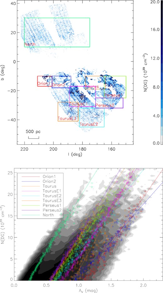
Upper panel: distribution of excess column densities. White areas are regions where no suitable extinction or H i data are available, and regions where the CO emission is so intense such that WCO > 1 K km s− 1. The squares delineate the different regions analysed in the current work. The map has an angular resolution of 6 arcmin. Lower panel: correlation between the visual extinction AV and the DG column density. Pluses of different colours are binned median values for the different regions, whereas lines of different colours are linear fits to the binned median values.
6 SUMMARY
In this paper, we have constructed a 2D extinction map integrated out to a distance of 4 kpc for the footprint of XSTPS-GAC using the data presented in Paper I. The map has a high angular resolution of 6 arcmin and a low noise level of 0.18 mag in AV [∼60 mmag in E(B − V)]. A comparison with the widely used SFD dust map and the newly derived Schlafly et al. (2014) reddening map shows that our map has a high fidelity.
The integrated extinction map is combined with high-resolution |${\rm H\,\small {i}}$| and CO measurements to study the correlation between the interstellar gas content and dust extinction within the XSTPS-GAC footprint. The main results are as follows.
An average value of dust-to-gas ratio DGR = (4.15 ± 0.01) × 10− 22 mag cm2 and an average CO-to-H2 conversion factor XCO = (1.72 ± 0.01) × 1020 cm− 2 (K km s− 1)− 1 are found for the XSTPS-GAC footprint of |b| > 10°. The results are consistent with the findings of previous work.
We find a factor of ∼ 2 cloud-to-cloud variations in the values of DGR and XCO amongst the molecular clouds south of the Galactic plane within the XSTPS-GAC footprint. Variations of DGR could partly be caused by the differences in dust properties, such as the grain size distribution of the different clouds. The XCO values found for the molecular clouds are around ∼ 1.5 × 1020 cm− 2 (K km s− 1)− 1, in close agreement with the work of Polk et al. (1988).
We find a range of DG mass fraction similar to those found by Planck Collaboration XIX et al. (2011) and by Paradis et al. (2012). The mass of DG is about 23 and 124 per cent those of the atomic and the CO-traced molecular gas, respectively. The fraction of molecular mass of the component, fDG, is about 0.55. The ‘close’ agreement between results from different analyses, which utilize different data set of differing spatial resolutions and sky coverage, probably indicates a ‘true universal’ fraction of DG mass relative to that of all gas, which is ∼20 per cent on large Galactic scale. Amongst the different clouds, fDG decreases with increasing average extinction. Our DG mass estimates are much larger than that modelled in Wolfire et al. (2010) but quite consistent with the theoretical work of Papadopoulos et al. (2002). In addition, we find that the DG column density has a linear relationship with the visual extinction. The average DG-to-dust ratio N(DG)/AV is ∼ 2.0 × 1021 cm− 2 mag− 1. The extinction of the H i-to-H2 transition layer varies between 0.22 and 1.10 mag, and increases with increasing average extinction of the cloud.
We thank the anonymous referee for instructive comments that improved the current work significantly. This work is partially supported by National Key Basic Research Program of China 2014CB845700 and China Postdoctoral Science Foundation 2014M560843.
This work has made use of data products from the Guoshoujing Telescope (the Large Sky Area Multi-Object Fibre Spectroscopic Telescope, LAMOST). LAMOST is a National Major Scientific Project built by the Chinese Academy of Sciences. Funding for the project has been provided by the National Development and Reform Commission. LAMOST is operated and managed by the National Astronomical Observatories, Chinese Academy of Sciences.
This publication utilizes data from Galactic ALFA H i (GALFA-HI) survey data set obtained with the Arecibo L-band Feed Array (ALFA) on the Arecibo 305-m telescope. Arecibo Observatory is part of the National Astronomy and Ionosphere Center, which is operated by Cornell University under Cooperative Agreement with the U.S. National Science Foundation. The GALFA-HI surveys are funded by the NSF through grants to Columbia University, the University of Wisconsin, and the University of California.
LAMOST fellow.
http://162.105.156.249/site/ Photometric-Extinctions-and-Distances.
