


Abstract
In recent years, compact jets have been playing a growing role in the understanding of accreting black hole engines. In the case of X-ray binary systems, compact jets are usually associated with the hard state phase of a source outburst. Recent observations of GX 339-4 have demonstrated the presence of a variable synchrotron spectral break in the mid-infrared band that was associated with its compact jet. In the model used in this study, we assume that the jet emission is produced by electrons accelerated in internal shocks driven by rapid fluctuations of the jet velocity. The resulting spectral energy distribution (SED) and variability properties are very sensitive to the Fourier power spectrum density (PSD) of the assumed fluctuations of the jet Lorentz factor. These fluctuations are likely to be triggered by the variability of the accretion flow which is best traced by the X-ray emission. Taking the PSD of the jet Lorentz factor fluctuations to be identical to the observed X-ray PSD, our study finds that the internal shock model successfully reproduces the radio to infrared SED of the source at the time of the observations as well as the reported strong mid-infrared spectral variability.
1 INTRODUCTION
Decades after their discovery, the fine details of the mechanisms behind jet formation and its connection to the accretion disc are still unclear. Revealing the disc–jet connection would help answer major questions concerning accreting black holes of all sizes, their growth and the role they play in galaxy evolution.
Conical compact jet models have been successful in reproducing the flat or slightly inverted radio spectra usually seen in X-ray binary sources (Corbel et al. 2000; Fender et al. 2000; Corbel & Fender 2002). However, they all require a dissipation process to compensate for adiabatic losses (Blandford & Königl 1979). One proposed process is the conversion of jet kinetic energy to internal energy through internal shocks.
Internal shock jet models have been proposed to describe the multiwavelength emission from γ-ray burst (Rees & Meszaros 1994; Daigne & Mochkovitch 1998), active galactic nuclei (Rees 1978; Spada et al. 2001; Böttcher & Dermer 2010) and microquasars (Kaiser, Sunyaev & Spruit 2000; Jamil, Fender & Kaiser 2010; Malzac 2013). One key point of these models is that their resulting spectral energy distributions (SED) are very sensitive to the shape of the assumed fluctuations of the jet velocity (Malzac 2014). Malzac (2013) has shown that internal shocks powered by flicker noise fluctuations of the bulk Lorentz factor can entirely compensate for the adiabatic expansion losses. Interestingly, the X-ray power spectrum of X-ray binaries, which traces the variability of the accretion flow in the vicinity of the compact object, is close to a flicker noise process (Lyubarskii 1997; King et al. 2004; Mayer & Pringle 2006).
GX 339-4 is a recurrent X-ray transient and the system is a confirmed black hole X-ray binary with a low-mass companion star. Although the black hole mass, the system inclination angle and distance are still unknown, they range between 5.8 and 10 M⊙ (Hynes et al. 2003; Muñoz-Darias, Casares & Martínez-Pais 2008; Shidatsu et al. 2011), 20° and 50° (Miller et al. 2006; Done & Diaz Trigo 2010; Shidatsu et al. 2011) and 6 and 15 kpc (Hynes et al. 2004; Zdziarski et al. 2004; Shidatsu et al. 2011), respectively. The source exhibits multiwavelength variability on a broad range of time-scales (Motch, Ilovaisky & Chevalier 1982; Fender, Hanson & Pooley 1999; Corbel et al. 2003, 2013; Dunn et al. 2008; Gandhi 2009; Casella et al. 2010). In addition, it also shows evidence of relativistic jets (Fender et al. 1997; Corbel et al. 2000; Markoff et al. 2003; Gandhi et al. 2008). The observations we used in this work are part of a multiwavelength study of GX 339-4 (Cadolle Bel et al. 2011; Corbel et al. 2013), and in particular of the first mid-infrared study of the source published in Gandhi et al. (2011) and obtained on 2010 March 11. GX 339-4 was observed with theWide-field Infrared Survey Explorer (WISE; Wright et al. 2010) satellite in four bands (1.36 × 10¹³, 2.50 × 10¹³, 6.52 × 10¹³ and 8.82 × 10¹³ Hz, respectively, W4, W3, W2 and W1), at 13 epochs, sampled at multiples of the satellite orbital period of 95 min and with a shortest sampling interval of 11 s, when WISE caught the source on two consecutive scans. Radio data were obtained with the Australian Telescope Compact Array during two days – close to but not simultaneous with WISE data – on 2010 March 7 and 14. The mean fluxes are 9.1 ± 0.1 and 9.7 ± 0.1 mJy at 5.5 and 9 GHz, respectively. X-ray data were quasi-simultaneous with WISE, taken between epochs 12 and 13 with the Rossi X-ray Timing Explore (RXTE) satellite. Gandhi et al. (2011) confirm the detection in the mid-infrared of a synchrotron break associated with the compact jet in GX 339-4 (Corbel & Fender 2002), and report the first clear detection of its strong variability. This detection of the jet's intrinsic variability and the overall properties of GX 339-4 make it the ideal source to test our model.
The objective of this paper is to determine whether an internal shock jet model driven by accretion flow variability reproduces spectral and timing observations of an X-ray binary source in the hard spectral state, known to be associated with compact jets. Our work differs from previous internal shock jet models in that we use the observed X-ray power spectral density (PSD) of the studied source, GX 339-4, to constrain the fluctuations of the bulk Lorentz factor γ of the ejecta constituting the jet. In Section 2, we introduce the internal shock jet model used to perform our simulations and the assumptions chosen to model the source. Sections 3 and 4 present the spectral and timing analyses carried out during this study, and the results obtained. We conclude this paper with a discussion of these results and suggestions for future developments in Section 5.
2 INTERNAL SHOCK MODEL
Malzac (2014) presents a newly developed numerical code which simulates the hierarchical merging and the emission of ejecta constituting a jet. In this model, a new shell of gas is ejected at each time step Δt, comparable to the dynamical time-scale at rdyn, the initial radius of the ejecta. The Lorentz factor of each shell varies, depending on the time of ejection. Its fluctuation follows a specified PSD shape. Throughout the duration of the simulation, the injected shells – and any subsequent shells resulting from mergers – are tracked until they interact and merge with other ejecta. The ejecta lose internal energy via adiabatic losses when propagating outwards. However, during mergers, a fraction of their kinetic energy is converted into internal energy. The details of the physics and the description of the main parameters of the model are presented in the original paper. The aim of this study is to investigate the possibility to reproduce GX 339-4 broad-band spectra and infrared light curves measured in Gandhi et al. (2011) with such a jet model, using the X-ray PSD as input for the fluctuations of the bulk Lorentz factor γ of the jet.
Following Gandhi et al. (2011), we take as initial parameters representative of the source, a mass of the central object of 10 M⊙ and a distance of 8 kpc (Zdziarski et al. 2004; Shidatsu et al. 2011). We let our simulations run for tsimu = 105 s (∼1 d), to allow the jet to develop. Due to the uncertainty on the inclination angle θ, we examine different values between 20° and 50°. We set the jet opening angle ϕ to 1°. We simulate a counter-jet in this study, however, its contribution to the total SED is less than 10 per cent in the energy range of interest.
Gandhi et al. (2011) report an X-ray luminosity during the observations of L2–10 keV = 2.0 × 1037 erg s−1. As a consequence, we estimate the total power of the jet during the observations to be Pjet ≃ 0.05 LEdd.
Finally, the most important parameter of our model is the distribution of the fluctuations in the jet's bulk Lorentz factor. We choose for the distribution of the fluctuations of the kinetic energy γ − 1 to follow the shape of GX 339-4 quasi-simultaneous X-ray PSD, observed by RXTE and shown in Fig. 1, as X-ray PSD is thought to trace the variability of the accretion flow in X-ray binary sources. Moreover, the fractional rms amplitude of γ − 1 is set to be equal to that of the X-ray PSD, in this case 35.6 per cent. By imposing the distribution of the fluctuations of the jet's bulk Lorentz factor to follow the X-ray PSD, we connect the physics of the jets to the variability of the inner part of the accretion flow.
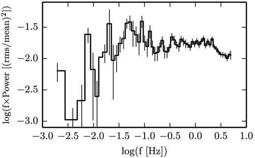
X-ray PSD of GX 339-4 in the 3–20 keV band, used to constrain the fluctuations of the bulk Lorentz factor of the ejecta. The PSD was extracted for the RXTE PCA observations with ObsId 95409-01-09-03 which was quasi-simultaneous with WISE (goodtime exposure ∼1360 s). Standard procedures were used for computing the PSD (for details, see section 4.2 of Gandhi et al. 2010).
In order to find the preferred set of parameters which accurately reproduces the broad-band spectra of the source, we have investigated the following parameters of the model: the mean jet Lorentz factor γmean, the electron and proton equipartition factors ξe and ξp, the ejecta scheme and the shock propagation scheme. γmean sets the amplitude of the overall spectra. The model provides three methods to generate the ejected shells: the ejecta have either a constant kinetic energy, or a constant mass, or their masses randomly vary, following the same distribution as the Lorentz factor's fluctuations. The ejecta scheme with constant shell mass provides the most pronounced bimodal behaviour of the correlation coefficients as observed by Gandhi et al. (2011). Therefore, we impose that scheme for the rest of the study. Finally, the shock propagation scheme is a parameter representing the two treatments available in the model of the energy dissipation occurring during a merger: a slow dissipation method, which overestimates the energy dissipation time, and a fast dissipation method, which underestimates the dissipation time-scale. These parameters, and their range, are listed in Table 1 .
Parameters explored.
| Parameters | Range of values |
|---|---|
| Inclination angle, θ | 20°, 30°, 40°, 45°, 50° |
| Mean Lorentz factor, γmean | 1.5, 2, 4 |
| Electron equipartition, ξe | 0.5, 1 |
| Proton equipartition, ξp | 0, 0.5, 1 |
| Ejecta scheme | Constant shell kinetic energy |
| constant shell mass | |
| random shell mass | |
| Shock propagation scheme | Slow, fast |
To assess the accuracy of our models in reproducing the spectral and timing observations of GX 339-4, we compared the simulated SED and infrared light curves to the data. The spectral and timing analyses performed and the results obtained are presented in the following sections.
3 SPECTRAL ANALYSIS
We use the internal shock model to generate different scenarios of jet formation and emission. The emission process considered in the model is solely synchrotron self-absorbed from non-thermal electrons. The electron distribution is a power law of spectral index p = 2.3, with its minimum and maximum energies (γmin and γmax) set arbitrarily and fixed throughout the simulation. The choice of p = 2.3 is driven empirically by the observed slope of the infrared spectrum interpreted as optically thin synchrotron radiation by a power-law energy distribution of electron (see Gandhi et al. 2011). This value of p is moreover consistent with a typical value expected in shock acceleration. The emission from every shell, initially injected as well as products of mergers, is calculated. The final SED, which is compared to the data, is the time-average of all these individual emissions over the simulation running time tsimu. The broad-band spectra are computed from 107 to 1016 Hz.
It is important to note that the general shape of the simulated SED is determined solely by the shape of the PSD used as an input to the fluctuations of the jet Lorentz factor. The explored parameters only allow us to modify the flux normalization or shift it in the photon frequency direction. Moreover, these parameters are degenerated, as two different sets of parameters can produce similar spectra. Hence, reproducing the overall shape of a observed spectra depends essentially on the shape imposed to the fluctuations of the jet's bulk Lorentz factor.
Fig. 2 compares the SED of our preferred model to the broad-band spectra of GX 339-4. The finding of this preferred set of parameters is done by an approximate match of the radio-to-infrared data. Despite the fact that no quantitative statistical fit has been carried out on the SED, we calculate a reduced-χ2 of 1.19 for 8 degrees of freedom [nine data points: two radio points, four WISE data points and the first three optical/ultraviolet (OUV) points, and one free parameter: inclination angle] for this particular set of parameters. When we do not consider the presence of a counter-jet, the reduced-χ2 lowers to 0.80. The significant difference in the reduced-χ2 values is mainly due to the higher contribution of the counter-jet to the radio points (∼10 per cent) compared to its contribution in the WISE bands (∼1 per cent). Five out of the nine data points used in the calculation of the reduced-χ2 do not include information on their variability over time. Consequently, the reduced-χ2 does not take into account the variance of flux in its calculation but only the error on each observed measurement. Taking into account the flux variability of the four WISE data points would decrease their contribution to the reduced-χ2 by approximately half and therefore would decrease as well the resulting reduced-χ2. It is apparent from this figure that we are capable of reproducing the overall shape of the radio-to-infrared observations with an internal shock model of jets powered with the accretion flow variability of the source. One should note that the OUV emissions are believed to originate from the outer parts of the accretion flow. We do not attempt to model this region. Finally, we do not model the X-ray emission that we attribute to the accretion flow. Instead, we use the X-ray emission as an upper limit to define the feasibility of our fit. We discuss the possible contribution of the jet to X-ray emission in Section 5.
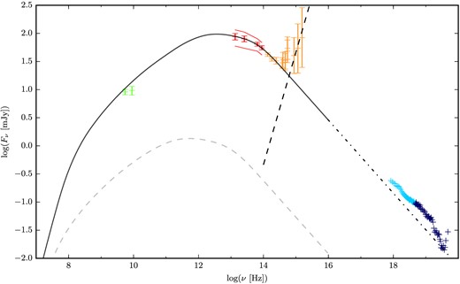
Broad-band spectra of our preferred model. Data points are from Gandhi et al. (2011). Radio points are plotted in green; WISE data in red; the near-infrared, optical and ultraviolet in orange; and the X-ray in blue. The radio points were obtained during two days, closest to but not simultaneous with WISE observations. The error bars represent the statistical and systematic errors on the mean. The total synchrotron self-absorbed jet emission from our model is shown as the solid black line. The contribution of the counter-jet is represented by the dashed grey line. Red curves represent the rms amplitude of variability over the 13 WISE epochs. The spectra have been averaged over the whole duration of the simulation. The dashed and dot–dashed black lines represent the contribution from the accretion disc to the spectra and the extrapolation of the optically thin synchrotron jet's emission, respectively. X-ray emission is used here solely as upper limits to define the feasibility of our fit.
The small discrepancy between the radio data points and our model can be partially explained by the fact that the radio observations were not performed simultaneously with WISE observations. In fact, if we use only the radio flux of the observation closest to the WISE observations (on 2010 March 14) instead of the mean of the two observations, then the model lies within the error bars of the radio points. The conical geometry assumed for the jet in this work may have an impact on the radio emission as well.
Table 2 presents the parameters of our preferred model. In bold are the parameters of the model, explored in our study. These parameters are consistent with the current knowledge we have on GX 339-4. However, due to the degenerate nature of the parameters, this fit is not unique. Nevertheless, the result does provide strong hints on the physical processes happening within the jet and its connection to the accretion flow variability.
Preferred model parameters.
| Parameters | Values |
|---|---|
| Mbh | 10 M⊙ |
| tsimu | 105 s |
| rdyn | 10 rG |
| Δt | 9.941 ms |
| ϕ | 1° |
| fvolumea | 0.7 |
| γab | 4/3 |
| |$\boldsymbol{\gamma _{\rm mean}}$| | 2 |
| PSD shape & amplitude | GX 339-4 X-ray PSD |
| (see Fig. 1) | |
| Ejecta scheme | Constant shell mass |
| Pjet | 0.05 LEdd |
| |$\boldsymbol{\xi _{{\rm e}}}$| | 1 |
| |$\boldsymbol{\xi _{{\rm p}}}$| | 0 |
| pc | 2.3 |
| γmin | 1 |
| γmax | 106 |
| |$\boldsymbol{\theta }$| | |$\boldsymbol{23^{\circ }}$| |
| Shock propagation scheme | Fast |
aVolume filling factor of the colliding shells.
bEffective adiabatic index of the flow.
cSpectral index of the electron distribution.
4 TIMING ANALYSIS
Following the finding of a preferred set of parameters, we compute the light curves of our preferred-model on time-scale of 11 s, at four infrared frequencies corresponding to the frequencies of WISE bands.
One important point should be noted here. On one hand, the internal shock jet model produces full light curves, from the beginning of the simulation to the end. On the other hand, WISE satellite produces a sampling of 11-s scans, at multiples of the satellite orbital period of 95 min. To enable a comparison between the simulations and the data, one needs to apply a mask reproducing the WISE scan of the source on the simulated light curves. By doing so, we obtain a set of 13-point light curves comparable to data.
To take into account the measurement uncertainties in these three characteristics, we used Monte Carlo bootstrapping to generate from each simulated light curve a collection of noised light curves. The noise added to each of the 13 epochs is drawn from a Gaussian distribution with a standard deviation equal to the errors on the individual WISE fluxes.
The infrared light curves are observables of a random variability process specific to the source. The WISE observations provide us with one realization of that process. Whereas the simulations provide us with many realizations, some of which are similar to the observations and some others are not. To determine whether our model statistically reproduces the observations, we investigate the distribution of simulated light curves. To that end, we use two kinds of estimators. As a first estimator, we compute the model distribution for each of the three characteristics |$F_{\nu ,W_{i}}$|, |$F_{{\rm var},W_{i}}$| and |$R_{W_{i}}^{W_{j}}$|.
Figs 3 –5 present the distributions of Fν, Fvar and R, respectively, of all the noised simulated light curves of our preferred model. Indicated in the figures by a red arrow is the position of the WISE observations within each distribution. In addition, the figure shows in grey area the 68 per cent variation around the median of the distribution, which would correspond to a ‘1σ’ variation if the distributions were Gaussian. To investigate if the WISE observations are typical in the framework of our model (our null-hypothesis), we evaluate the p-value of each observation characteristic. The p-value is the probability of obtaining a test statistic result at least as extreme as the one that was actually observed, assuming that the null hypothesis is true. For the flux and the fractional variability amplitude, the p-values are greater than 0.1 and we cannot reject our null-hypothesis. However, for the correlation coefficients of W4–W2, W4–W1 and W3–W1, the p-values are between 0.01 and 0.05. It suggests that our model does not fully reproduce the correlations seen between the bands with WISE. Indeed, the simulated light curves prove to be more deeply correlated than the observations. Nevertheless, it is interesting to note that the evolution of the mean values of the correlation coefficients R in Fig. 5 follows that of the observations. In the model, similar to the observations, bands W4 and W3 as well as W2 and W1 are the most correlated. Whereas W4 and W1 and W4 and W2 are the least correlated. Suggestions to explain the discrepancy in the correlation coefficients between the model and the observations are discussed in Section 5.

Distribution of Fν. The red arrow indicates the position of the observations. The green dashed line indicates the median of the distribution, the grey area represents the 1σ variation about the median.
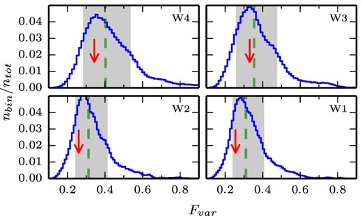
Distribution of Fvar. The red arrow indicates the position of the observations. The green dash line indicates the median of the distribution, the grey area represents the 1σ variation about the median.
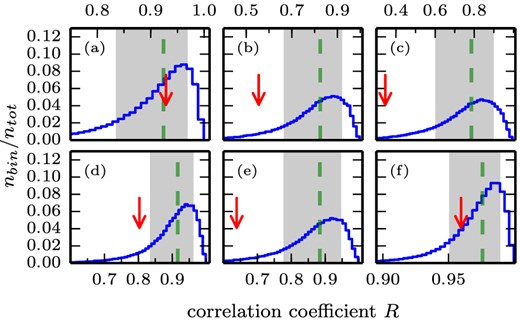
Correlation coefficient distributions of the simulated light curves of our preferred model. Comparing: (a) W4–W3, (b) W4–W2, (c) W4–W1, (d) W3–W2, (e) W3–W1 and (f) W2–W1. The red arrow indicates the position of the observations. The green dashed line indicates the median of the distribution, the grey area represents the 1σ variation about the median.
Fig. 6 presents a particular set of simulated light curves from our preferred model which have spectral as well as timing properties comparable to the WISE observations. That is, the simulated light curves shown here are the ones presenting simultaneously fluxes, variability and correlation coefficients closest to the red arrows indicated in Figs 3–5. Table 3 shows the values obtained for Fν, Fvar and R of that particular set of simulated light curves and compare them to those reported by Gandhi et al. (2011). In addition, the table reports the exact p-values obtained for each WISE characteristic.
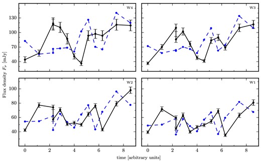
Selected set of light curves reproducing the observations: in blue dash, the simulated light curves, and in black solid, WISE light curves from Gandhi et al. (2011). The error bars represent the statistical and systematic errors.
Statistics of our preferred set of simulated light curves compared to those of the WISE observations.
| Simulation | WISE | p-value | ||
|---|---|---|---|---|
| Fν [mJy] | W1 | 54.63 | 55.2 ± 3.9 | 0.45 |
| W2 | 61.98 | 64.3 ± 4.6 | 0.33 | |
| W3 | 78.81 | 79.9 ± 7.3 | 0.47 | |
| W4 | 83.41 | 87.4 ± 8.3 | 0.47 | |
| Fvar | W1 | 0.24 | 0.25 ± 0.03 | 0.23 |
| W2 | 0.25 | 0.25 ± 0.03 | 0.24 | |
| W3 | 0.30 | 0.32 ± 0.06 | 0.44 | |
| W4 | 0.35 | 0.32 ± 0.06 | 0.36 | |
| R | W4–W3 | 0.97 | 0.93 | 0.47 |
| W4–W2 | 0.81 | 0.55 | 0.07 | |
| W4–W1 | 0.76 | 0.35 | 0.03 | |
| W3–W2 | 0.91 | 0.80 | 0.10 | |
| W3–W1 | 0.87 | 0.64 | 0.04 | |
| W2–W1 | 0.99 | 0.96 | 0.24 |
This quantity is similar to a reduced-χ2, with one important difference: the distribution of the characteristics are not Gaussian. The χ2 describes the match between the modelled and observed values of the three characteristics, exactly as it describes the match between the flux at different energies in usual spectral fitting for instance. As the model is intrinsically stochastic, we do not aim at reproducing accurately each single observation. Instead, we measure deviation of the observations to the model by comparing the statistical properties of those. As these characteristics are likely to be correlated, we use the inverse |$\bf{Q}$| of the covariance matrix to compute the χ2 rather than using the simpler expression for independent variables.
Fig. 7 presents two distributions of that quantity. On one hand, the reduced-χ2 was calculated considering the average flux and the fractional variability amplitudes only (top panel). On the other hand, it was calculated also including the correlation coefficients (bottom panel). The reduced-χ2 of the observations (represented by the red arrow) is equal to 0.71 and 1.89, respectively. The discrepancy between the model and the observations regarding the correlation coefficients reflects in the relatively high reduced-|$\chi ^{2}_{\rm obs}$| obtained when considering all three characteristics in its calculation. Alternatively, the lower reduced-|$\chi ^{2}_{\rm obs}$|, obtained when considering Fν and Fvar only, suggests that our model correctly reproduces the spectral and timing properties of the source at the time of the observations but does not reproduce the correlated nature of the bands. The p-values obtained for each case (0.38 and 0.08, respectively) suggest a similar conclusion.
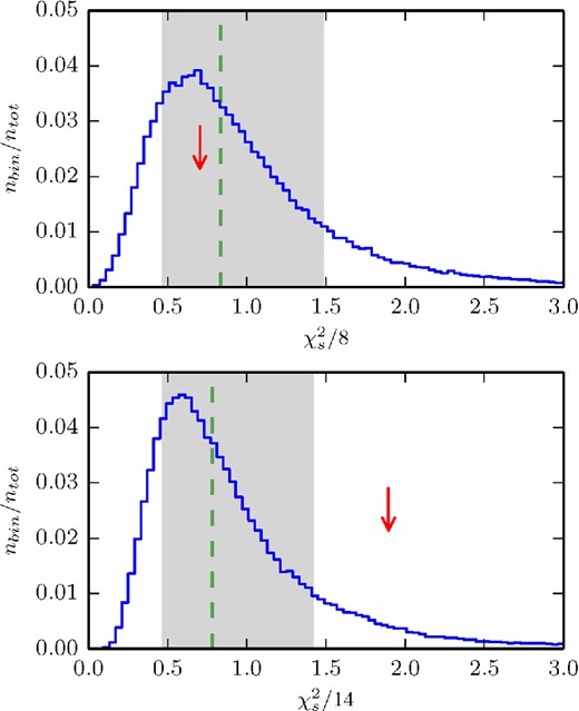
Distributions of reduced-|$\chi ^{2}_{{\rm s}}$|: (top) considering Fν and Fvar only; (bottom) considering Fν, Fvar and R. The red arrow indicates the position of the corresponding reduced-|$\chi ^{2}_{\rm obs}$|. The green dashed line indicates the median of the distribution, the grey area represents the 1σ variation about the median.
5 DISCUSSION
This work was designed to study the connection between the inner part of an accretion flow and the base of the corresponding launched outflow, in X-ray binary sources in the hard state. Using WISE observations of GX 339-4 from 2010 March 11, the results of this investigation show that it is indeed possible to reproduce simultaneously broad-band spectral and timing behaviour of a X-ray binary source in the hard state with an internal shock jet model. The required condition is to use the X-ray timing information provided by the corresponding PSD as an input to the fluctuations of the bulk Lorentz factor γ. This finding corroborates the ideas of Jamil et al. (2010) and Malzac (2014), who suggested that accretion flow variability, traced by X-ray timing information, could drive internal shock in jets.
Another point that could be investigated to characterize the disc–jet connection is the jet's contribution to the X-ray variability. Emission produced by the model at frequencies higher than 1016 Hz are currently extrapolated from the optically thin synchrotron power-law tail. However, several cooling processes, such as synchrotron self-Compton or inverse-Compton of the disc emission for example, are not considered in the model yet. Moreover, the form as well as the maximum energy of the emitting particle distribution are currently being fixed and arbitrarily set throughout the simulation. These restrictions lead to the choice of neglecting the possible contribution of the jet to the X-ray variability in the present state of the model.
Despite the more pronounced correlation in the simulated light curves compared to the observations, it is interesting to note the evolution of the spreading of the correlation coefficients R in Fig. 5 follows that of the observations. This tendency may be explained in terms of regions of emission. Fig. 8 illustrates this trend by showing that the regions of peak emission of W1 and W2 on one hand, and W3 and W4 on the other hand, are closely located, while the regions of peak emission of W1 and W4 are the most distant to each other. We may improve the correspondence between the correlation coefficients of the model and the observations by increasing the contribution of the counter-jet to the overall emission. This is done by releasing the constraint on the value of Pjet and increasing the inclination angle to 50°. We find a new fit to the SED by setting Pjet to 0.14 LEdd. However, that new choice of parameters does not enhance the overall fit (new reduced-χ2 is equal to 4.17) and ameliorates only slightly the correspondence between the correlation coefficients of the model and the observations.
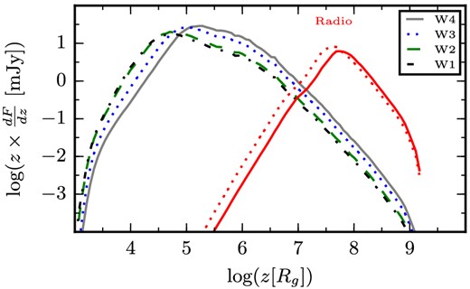
Regions of emission in the infrared and radio bands. In red, are the radio emission at 5.5 GHz (solid) and 9 GHz (dotted). In solid black, dotted blue, dashed green and dot–dashed black are the infrared emission in W4, W3, W2 and W1 bands, respectively.
The stronger correlation coefficients seen in the model, compared to those of the observation, are due to the regions of peak emission being so close to each other that a fluctuation occurring in one band does not have the time to be totally dissipated before arriving in the emitting region of the next band. To reduce the correlation between bands, one would need to allow the particles to cool on a faster time-scale or over a longer period of time. Improving the modelling of the particle distribution by taking into account radiative processes or modifying the geometry of the jet to consider amplified radial expansion at the shock lead by an increase of the internal pressure and possible radial contractions in between shock regions may adapt the cooling time-scale to that needed. Similarly, modifying the scale of the dissipation profile along the jet by changing the one-to-one relation between the accretion flow variability and the ejecta velocity distribution used in this study may provide a solution to that issue.
Nevertheless, it is important to note that this disagreement between the observed and modelled correlation coefficients does not challenge internal shocks as a dissipation process occurring in astrophysical jets. Such disagreement would appear in any model using any other dissipation process, as long as they also assume a jet of conical geometry and similar radiative treatment. Overall, investigating the variable properties of our model, improving the modelling of the particle distribution or modifying the geometry of the jet will shed some light on the origin of that dichotomy and will help to understand even better the deep relation between accretion and ejection processes in accreting black holes.
To conclude, this work is a step forward towards revealing the details of the accretion–ejection process in accreting black hole systems. The results of this study indicate that the conversion of jet kinetic energy to internal energy through internal shocks may well be the dissipation process needed to compensate for the adiabatic losses in conical compact jets. Furthermore, the results of this work support the idea of the importance of the X-ray variability on jet emission strength. A recent study by Dinçer et al. (2014) corroborates this idea. They observed that the standard sources in the radio/X-ray luminosity relation show stronger broad-band X-ray variability than outliers at a given X-ray luminosity. Further radio, mid-infrared and X-ray timing observations will provide better constraints to the accretion–ejection connection and to the present model. In addition, understanding and being able to reproduce the spectral, timing and correlation properties of a source will allow the model to provide useful predictions to future observations, with information such as at which frequency one can expect to observe maximum jet variability or at which time-scale is the best for probing it.
JM thanks the Institute of Astronomy (Cambridge) for hospitality. PG acknowledges support from STFC (grant reference ST/J003697/1). The authors are grateful to the anonymous referee for his/her helpful comments on the manuscript. This work is part of the CHAOS project ANR-12-BS05-0009 supported by the French Research National Agency (http://www.chaos-project.fr).
