


Abstract
We present an approach to the design of distribution functions that depend on the phase-space coordinates through the action integrals. The approach makes it easy to construct a dynamical model of a given stellar component. We illustrate the approach by deriving distribution functions that self-consistently generate several popular stellar systems, including the Hernquist, Jaffe, and Navarro, Frenk and White models. We focus on non-rotating spherical systems, but extension to flattened and rotating systems is trivial. Our distribution functions are easily added to each other and to previously published distribution functions for discs to create self-consistent multicomponent galaxies. The models this approach makes possible should prove valuable both for the interpretation of observational data and for exploring the non-equilibrium dynamics of galaxies via N-body simulations.
1 INTRODUCTION
Axisymmetric equilibrium models are extremely useful tools for the study of galaxies. A real galaxy will never be in perfect dynamical equilibrium – it might be accreting dwarf satellites, or being tidally disturbed by the gravitational field of the group or cluster to which it belongs, or displaying spiral structure – but an axisymmetric equilibrium model will usually provide a useful basis from which a more realistic model can be constructed by perturbation theory.
By Jeans (1915) theorem, every equilibrium model can be described by a distribution function (DF) that depends on the phase-space coordinates |$({\boldsymbol x},{\boldsymbol v})$| only through isolating integrals of motion. In an axisymmetric potential, most orbits prove to be quasi-periodic, with the consequence that they admit three isolating integrals (Arnold 1978). Consequently, a generic DF for an axisymmetric equilibrium galaxy is a function of three variables.
The major obstacle to exploiting this insight is that we have analytic expressions for only two isolating integrals of motion in a general axisymmetric potential, namely the energy |$E={\textstyle {1\over 2}}v^2+\Phi ({\boldsymbol x})$| and the component of the angular momentum about the symmetry axis, |$J_\phi =({\boldsymbol x}\times {\boldsymbol v})_z$|. Several authors have examined model galaxies with DFs of the two-integral form f(E, Jϕ) (Prendergast & Tomer 1970; Wilson 1975; Rowley 1988; Evans 1994), but in such models the velocity dispersions σR and σz in the radial and vertical directions are inevitably equal. This condition is seriously violated in our Galaxy and we have no reason to suppose that the condition is better satisfied in any external galaxy. Hence, it is mandatory to extend the DF's argument list to include a ‘non-classical’ integral, I3, for which we do not have a convenient expression.
To obtain the observable properties of a model defined by |$f({\boldsymbol J})$|, for example its density distribution |$\rho ({\boldsymbol x})=\int {\rm d}^3{\boldsymbol v}\,f({\boldsymbol J})$| and its velocity dispersion tensor |$\sigma ^2_{ij}({\boldsymbol x})$|, one has to be able to evaluate |${\boldsymbol J}({\boldsymbol x},{\boldsymbol v})$| in an arbitrary gravitational potential. Recently, a number of techniques have been developed for doing this (Binney 2012a; Sanders & Binney 2014, 2015). Consequently, while the last word on action evaluation has likely not yet been written, we now have algorithms that enable one to extract the observables from a DF |$f({\boldsymbol J})$| with reasonable accuracy.
DFs |$f({\boldsymbol J})$| that depend on the phase-space coordinates only through the actions were first used to model the disc of our Galaxy in an assumed gravitational potential (Binney 2010, 2012b). Recently, Binney (2014, hereafter B14) showed how to derive the self-consistent gravitational potential that is implied by a given |$f({\boldsymbol J})$| by exploring a family of flattened, rotating models that he derived from the ‘ergodic’ DF of the isochrone model: that is the DF f(H) that depends on the phase-space coordinates only through the Hamiltonian |$H=\frac{1}{2} v^2+\Phi ({\boldsymbol x})$|. Hénon (1960) derived the isochrone's ergodic DF, and in the case of the isochrone potential explicit expressions are available for |${\boldsymbol J}({\boldsymbol x},{\boldsymbol v})$| and |$H({\boldsymbol J})$| (Gerhard & Saha 1991). Substituting |$H({\boldsymbol J})$| in f(H) B14 obtained the DF |$f({\boldsymbol J})$| of the isotropic isochrone model. In this paper, we present simple analytic functions |$f({\boldsymbol J})$| that generate nearly isotropic models of other widely used models, such as the Hernquist (1990), Jaffe (1983), and Navarro, Frenk & White (1996, hereafter NFW) models.
Once a DF of the form |$f({\boldsymbol J})$| is available for a spherical, non-rotating model, the procedure B14 used to flatten the isochrone sphere and to set it rotating can be used to flatten and/or set rotating one's chosen model. So DFs for spherical models in the form |$f({\boldsymbol J})$| are valuable starting points from which quite general axisymmetric models are readily constructed.
Galaxies are generally considered to consist of a number of components, such as a disc, a bulge, and a dark halo, that cohabit a single gravitational potential. If we represent each component by a DF of the form |$f({\boldsymbol J})$|, it is straightforward to find the gravitational potential in which they are all in equilibrium (e.g. Piffl et al. 2014; Piffl, Penoyre & Binney in preparation). An analogous composition using DFs of the form f(E, Jϕ, I3) has never been achieved and may be impossible, because when components are added, their potentials must be added, and the energies of physically similar orbits in a given component are quite different before and after we add in the potential of another component. For example, the orbit on which a star sits at the centre of the galaxy will have different energies before and after addition. If E is used as an argument of the DF, the change in E will change the density of stars on the given orbit, which is contrary to the fundamental idea of building up the galaxy by adding components. By contrast, the actions of the orbit on which a star sits at the galactic centre vanish in any potential, and if a component is defined by |$f({\boldsymbol J})$|, it contributes the same density of stars to this orbit regardless of the external potential in which that component finds itself. This fact is a major motivation for discovering what DF of the form |$f({\boldsymbol J})$| is required to generate each component of a galaxy.
The DF of an isotropic spherical model must depend on the actions only via the Hamiltonian |$H({\boldsymbol J})$|. The dependence of f on H is readily obtained from the inversion formula of Eddington (1916), but an exact expression for |$H({\boldsymbol J})$| is only available for the isochrone potential and its limiting cases, the harmonic oscillator and Kepler potentials. Our ignorance of |$H({\boldsymbol J})$| for potentials other than the isochrone amounts to a barrier to the extension of B14's approach to model building. One way to break through this barrier is to devise numerical approximations to |$H({\boldsymbol J})$| and some success has been had in this direction by Fermani (2013) and Williams, Evans & Bowden (2014). In this paper, we pursue a slightly different strategy, which is to develop simple algebraic expressions for DFs |$f({\boldsymbol J})$| that generate self-consistent models that closely resemble popular spherical systems. We also show that a very simple form of |$f({\boldsymbol J})$| generates a model that is almost identical to the isochrone sphere and we give a useful analytic expression for the radial action as a function of energy and angular momentum for a Hernquist sphere.
The paper is organized as follows. In Section 2, we use analytic arguments to infer |$f({\boldsymbol J})$| for scale-free models. These models are not physically realizable as they stand, so in Section 3 we consider models that consist of two power-law sections joined at a break radius. In Section 4, we extract realizable models from scale-free models by the alternative strategy of adding a core to the system and/or tidally truncating the model. Section 5 sums up.
2 POWER-LAW MODELS
Consider a gravitational potential that scales as a power of the distance from the galactic centre, i.e. |$\Phi (\xi {\boldsymbol x})\propto \xi ^a\Phi ({\boldsymbol x})$| with |$a\not= 0$|: in the limit a → 0 the gravitational potential tends to a logarithmic potential, which is an interesting special case that we will treat in Section 2.1.
In the definition (10) of |$h({\boldsymbol J})$|, the modulus of the angular momentum Jϕ appears because we are concerned with the construction of the part of the DF that is even in Jϕ. If we wish to set the model rotating, we will add to this even part an odd part as discussed by B14.
2.1 Logarithmic potentials
Note that equation (24) implies that the phase-space density diverges as |${\boldsymbol J}\rightarrow 0$|. It follows that this DF unambiguously specifies the singular isothermal sphere, in contrast to the DF (23), from which one can derive both cored and singular isothermal spheres (e.g. Binney & Tremaine 2008, section 4.3.3b). It is characteristic of DFs of the form |$f({\boldsymbol J})$| that they uniquely and transparently specify the phase-space density both at the centre of the model (|${\boldsymbol J}=0$|) and for marginally bound orbits |$({\boldsymbol J}\rightarrow \infty )$|. From a DF that depends on energy, by contrast, the phase-space density at the centre of the model is implicitly specified by the boundary condition adopted at r = 0 when solving Poisson's equation for the self-consistent potential.
The considerations of the last paragraph apply equally to the power-law DFs (16): although we used the standard form (15) of the energy-based DF of the polytropes to derive this DF, it implies infinite phase-space density at the system's centre, so it is inconsistent with familiar cored polytropes, such as the Plummer model.
3 TWO-POWER MODELS
The DF (34) is infinite on the orbit |${\boldsymbol J} = 0$| of a star that is stationary at the model's centre. Cuspy models such as the Hernquist, Jaffe and NFW models do have such centrally divergent DFs, while in other cored systems the phase-space density reaches a finite maximum. Cored systems will be treated in Section 4.
3.1 Technicalities
The ratio of the half-mass radius rh to the scale radius r0, defined by equation (38), for the |$f({\boldsymbol J})$| isochrone, |$f({\boldsymbol J})$| Hernquist and |$f({\boldsymbol J})$| Jaffe models. For comparison, we list also the ratio rh/rb, where rb is the break radius, of the corresponding classical models.
| Isochrone | Hernquist | Jaffe | |
|---|---|---|---|
| rh/r0 | 3.4 | 2.42 | 0.76 |
| rh/rb | 3.06 | 2.41 | 1 |
| Isochrone | Hernquist | Jaffe | |
|---|---|---|---|
| rh/r0 | 3.4 | 2.42 | 0.76 |
| rh/rb | 3.06 | 2.41 | 1 |
Once |$f({\boldsymbol J})$| has been normalized, we are able to determine the potential |$\Phi ({\boldsymbol x})$| that the model self-consistently generates by the iterative procedure described by B14.
3.2 Worked examples
3.2.1 The Hernquist model
The Hernquist (1990) model is an interesting example both because it is a widely used model and because we can derive its ergodic DF as a function of the actions for comparison with the |$f({\boldsymbol J})$| model given by equation (34) with (α, β) = (1, 4), which hereafter we refer to as |$f({\boldsymbol J})$| Hernquist model.
In Appendix A, we derive an analytic expression for Jr = Jr(H, L) in the spherical Hernquist potential. By numerically inverting this expression, we arrive at H = H(Jr, L) for the Hernquist sphere. Combining this with the sphere's ergodic DF, which was given already by Hernquist (1990), we have the exact |$f=f[H({\boldsymbol J})]$|. In Fig. 1, we show surfaces in action space on which this DF is constant together with surfaces on which DF of the |$f({\boldsymbol J})$| Hernquist model is constant. The differences are small but apparent and arise because the surfaces of constant energy are not exactly planar.
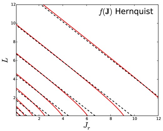
The red full curves show surfaces on which the DF of the classical isotropic Hernquist sphere is constant in the (Jr, L) plane of action space, while the black dashed curves show surfaces on which the corresponding |$f({\boldsymbol J})$| DF is constant.
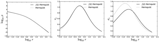
Density (left-hand panel), circular velocity (central panel), and radial velocity dispersion (right-hand panel) profiles for the classical isotropic Hernquist sphere (normalized to rb) and for the |$f({\boldsymbol J})$| Hernquist model (normalized to r0).

3.2.2 The Jaffe model
The Jaffe (1983) model behaves as Hernquist's at large radii, while tending to ρ ∝ r−2 close to the centre. Fig. 4 shows the radial profiles of the |$f({\boldsymbol J})$| Jaffe model defined by setting (α, β) = (2, 4) in the DF (34), and compares them with the classical isotropic model. The discrepancies in σr are due to the slight radial bias of the |$f({\boldsymbol J})$| model around r0. The full curve in Fig. 3 shows that this bias is actually quite mild – |βa| < 0.1.
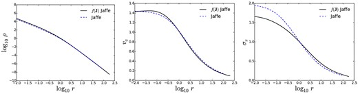
Same as Fig. 2, but for the classical isotropic Jaffe sphere and for the |$f({\boldsymbol J})$| Jaffe model.
3.2.3 NFW halo

4 CORES AND CUTS
4.1 Isochrone model
Fig. 6 compares the density profiles of the model equation (42) generates for β = 4 (black curves) with those of the isochrone (Hénon 1960). The two models are extremely similar, so we shall refer to the model generated by the DF (42) when β = 4 as the |$f({\boldsymbol J})$| isochrone model. The density profiles of the two models are essentially identical, but at r ≃ r0 σr is slightly smaller in the |$f({\boldsymbol J})$| isochrone than in the classical isochrone because the |$f({\boldsymbol J})$| isochrone is mildly radially biased near r0 – the thin full curve in Fig. 3 shows βa(r) for this model. It is non-zero because action space surfaces of |$f({\boldsymbol J})$| do not quite coincide with surfaces of constant |$H({\boldsymbol J})$|, as the upper panel of Fig. 7 shows by plotting contours of f and H. For the isochrone potential, we have an analytic expression for the frequency ratio Ωϕ/Ωr as a function of L. The lower panel of Fig. 7 shows that the constant-energy and constant-DF contours are more closely aligned when the argument of the homogeneous function uses the exact frequency ratio.
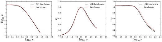
Same as Fig. 2, but for the classical isotropic isochrone sphere and for the |$f({\boldsymbol J})$| isochrone model.
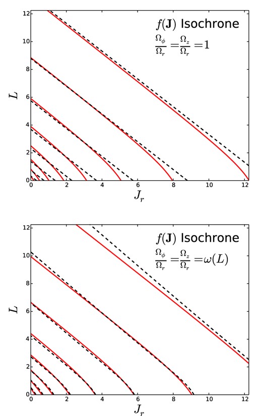
Surfaces of constant |$H({\boldsymbol J})$| (red) and of constant |$f({\boldsymbol J})$| black in action space for two |$f({\boldsymbol J})$| isochrone models with different choice of the function g appearing in the DF (42). In the upper panel, g is Jr + L whereas in the lower panel it is Jr + (Ωϕ/Ωr)L where the frequency ratio is a function of L.
Given that the exact DF of the isochrone is a complicated function of |${\boldsymbol J}$|, it is astonishing that the trivial DF (42) provides such a good approximation to it.
4.2 Cored isothermal sphere

5 CONCLUSIONS
Studies of both our own and external galaxies will benefit from the availability of a flexible array of dynamical models of galactic components such as disc, bulge and dark halo. The construction of general models of this type is rather straightforward when one decides to start from an expression for the component's DF as a function of the action integrals Ji. In this paper, we have illustrated this fact by deriving simple analytic forms for DFs that self-consistently generate models that closely resemble the isochrone, Hernquist, Jaffe, NFW and truncated isothermal models. In previous papers, Binney (2010, 2012b) has given simple analytic DFs that provide excellent fits to the structure of the Galactic disc, so now DFs are available for all commonly occurring galactic components.
Our models are tailored to minimize velocity anisotropy at both small and large radii. In all of them, the anisotropy parameter βa peaks at intermediate radii. The peak is by far sharpest in the |$f({\boldsymbol J})$| isochrone, but even in this model βa stays below 0.25.
Our presentation has been elementary in the sense that we have confined ourselves to spherical, almost isotropic components that live in isolation. However, B14 showed that given a near-ergodic DF |$f({\boldsymbol J})$| of a component such as those presented here, it is trivial to modify it so it generates a system that is flattened by velocity anisotropy, or by rotation, or by a combination of the two. Equally important, when the DF of an individual component is given as |$f({\boldsymbol J})$|, it is straightforward to add components. Such addition was exploited by Piffl et al. (2014) in a study of the contribution of dark matter to the gravitational force on the Sun: in that study the models fitted to data comprised a sum of DFs |$f({\boldsymbol J})$| for the disc and the stellar halo. The dark halo was assigned a density distribution rather than a DF, but Piffl et al. (in preparation) represent the dark halo by the |$f({\boldsymbol J})$|NFW model, making the Galaxy a completely self-consistent object. A key point for such work is that the mass of each component can be specified at the outset.
Our approach has several points of contact with that of Williams et al. (2014) and Evans & Williams (2014), who derive approximations to |$H({\boldsymbol J})$| for models that are defined by DFs of the form f(E, L). In particular, they show that for their models better approximations to the iso-energy surfaces in action space can be obtained if one's homogeneous function has as its argument the sum of a linear function of the actions, as used here, and a small term |$\epsilon \sqrt{LJ_r}$|. We expect that the anisotropy of our models could be enhanced by adding such a term.
In addition to assisting in the dynamical interpretation of observations of galaxies, the models that this work makes possible could provide useful initial conditions for N-body simulations. The first step would be the construction of a self-consistent galaxy model from a judiciously chosen DF. Then one could Monte Carlo sample the action space using the DF as the sampling density, and torus mapping (e.g. Binney & McMillan 2011) could be used to generate an orbital torus at each of the selected actions. Finally, some number n of initial conditions |$({\boldsymbol x},{\boldsymbol v})$| would be selected on each torus, uniformly space in the angles θi. The resulting simulation would be in equilibrium to whatever precision had been used in the solution of Poisson's equation, and it would experience a ‘cold start’ (Sellwood 1987). Moreover, given that it would be possible to evaluate the original DF at any phase-space point, the model would lend itself to the method of perturbation particles (Leeuwin, Combes & Binney 1993) in which the simulation particles represent the difference between a dynamically evolving model and an underlying equilibrium rather than the whole model. This method has been little used in the past on account of the lack of interesting models with known DFs, which is precisely the need that we have here supplied.
LP is pleased to thank the Rudolf Peierls Centre for Theoretical Physics in Oxford for the warm hospitality during an early phase of this work. JB is supported by the European Research Council under the European Union's Seventh Framework Programme (FP7/2007-2013)/ERC grant agreement no. 321067, and by the UK Science Technology through grant ST/K00106X/1. LC and CN are partly supported by PRIN MIUR 2010-2011, project ‘The Chemical and Dynamical Evolution of the Milky Way and Local Group Galaxies’, prot. 2010LY5N2T.
In the non-spherical case,
