


Abstract
In the solar neighbourhood, there are moving groups of stars with similar ages and others of stars with heterogeneous ages as the field stars. To explain these facts, we have constructed a simple model of three phases. Phase A: a giant interstellar cloud is uniformly accelerated (or decelerated) with respect to the field stars during a relatively short period of time (10 Myr) and the cloud's mass is uniformly increased. As a result, a number of passing field stars is gravitationally captured by the cloud at the end of this phase; phase B: the acceleration (or deceleration) and mass accretion of the cloud cease. The star formation spreads throughout the cloud, giving origin to stellar groups of similar ages; and phase C: the cloud loses all its gaseous component at a constant rate and in parallel is uniformly decelerated (or accelerated) until reaching the initial velocity of phase A (case 1) or the velocity of the gas cloud remains constant (case 2). Both cases give equivalent results. The system equations for the star motions governed by a time-dependent gravitational potential of the giant cloud and referred to a coordinate system comoving with the cloud have been solved analytically. We have assumed a homogeneous spheroidal cloud of fixed semimajor axis a = 300 pc and of an initial density of 7 atoms cm− 3, with a density increment of 100 per cent and a cloud's velocity variation of 30 km s−1, from the beginning to the end of phase A. The result is that about 4 per cent of the field stars that are passing within the volume of the cloud at the beginning of phase A are captured. The Sun itself could have been captured by the same cloud that originated the moving groups of the solar neighbourhood.
1 INTRODUCTION
An important problem of Galactic dynamics is the formation of the moving stellar groups, and in particular, of those located in the solar neighbourhood. The existence of kinematic groups of stars, used to be called star streams, was recognized after the pioneering studies of Proctor (1869) and the theory of the two star streams of Kapteyn (1905) that was a fundamental step for the development of the Galactic dynamics (for an historical survey on this topic see Antoja et al. 2010). The peculiarity of the moving groups is that even though they are gravitationally unbound systems subject to the tidal disruption, the members of each group have shared a very similar spatial velocity for a long time. An explanation could be that these stellar groups are relics of an old star-forming event (Eggen 1965, 1995, 1996; Asiain, Figueras & Torra 1999) and that they have been tied to the mother gas-cloud, until it has been dispersed (Olano 2001). The existence of groups chemically homogeneous seems to support this hypothesis (De Silva et al. 2007). However, there are other groups that cannot be chemically distinguished from the field stars (Bensby et al. 2007). Another mechanism for forming moving groups involves orbital resonance effects due to the bar and/or the spiral arms of the Galaxy (Dehnen 1998; Fux 2001; Antoja et al. 2011; Quillen et al. 2011).
Certainly, this mechanism can explain the age heterogeneity observed in certain moving groups (De Simone, Wu & Tremaine 2004; Famaey et al. 2005; Famaey, Siebert & Jorissen 2008). Hence, the two models are not incompatible or mutually exclusive, but it would imply that groups originated by two different mechanisms coexist in the solar vicinity.
In this paper, we propose a sole mechanism that could account for both kinds of moving groups: homogeneous and heterogeneous in age. We will demonstrate that the sudden acceleration (or deceleration) of a giant interstellar cloud plus an increment of the cloud mass during the processes is an efficient mechanism to capture field stars passing on the gas cloud. This mechanism favours the capture of stars with velocities similar to the cloud's peculiar velocity produced by the acceleration process. It would explain the formation of moving groups of field stars. The Sun itself would been captured by the cloud that gave origin to the local moving groups (Olano 2001). On the other hand, the formation of stars within the giant gas cloud gave origin to stellar groups of similar ages.
The giant H i clouds (or superclouds), with typical radii of a few hundred parsecs, are observed mainly in and close to the spiral arms of the Galaxy (Elmegreen & Elmegreen 1987). According to the theory of density waves, the gas clouds are comprised and strongly decelerated when they enter the spiral density wave (Roberts 1969, 1970). Another phenomenon that can accelerate gas of huge regions of the Galactic disc and form such giant clouds is the fall of high-velocity clouds (HVCs) on the Galactic disc (see Olano 2004, 2008 and references therein).
Previous studies have been focused on the capture of field stars by molecular clouds (Bhatt 1989) and by collapsing clouds (Whitman, Matese & Whitmire 1991). In both studies, the clouds taken as a whole have been considered at rest with respect to the field stars.
This work is organized in the following manner. In Section 2, we develop a model in which a giant interstellar cloud whose mass and kinematics are subject to abrupt changes is able to capture a percentage of the field stars that are passing through the cloud. The movements of stars under a time-variable gravitational potential of a homogeneous oblate spheroid, representing the cloud, are referred to a coordinate system joined to the cloud which moves with a constant linear acceleration, and the corresponding motion equations are solved analytically (Section 2.1). We derive the velocity distribution of the field stars lying within the cloud at the beginning of the process, providing the initial conditions to derive the orbits of the stars (Section 2.2), and determine the stars that are captured (Section 2.3). In Section 3 and its subsections, we present the results, including the possible capture of the Sun by the same interstellar cloud that originated the local moving groups (Section 3.4) and the formation of moving groups of stars born in the cloud (Section 3.5). Finally, in Section 4, we give the conclusions of this work.
2 THE MODEL
The model starts with a gaseous protocloud in which there are field stars passing through the cloud with velocities greater than the escape velocity. Then, the cloud, originally at rest in the local standard of rest (LSR) within the cloud's neighbourhood, is accelerated (or decelerated) during certain time in which the cloud also grows its mass by accretion of the surrounding gas. We will call this period phase A. We will show that at the end of phase A a number of the passing field stars are trapped by the cloud. That is to say that their resulting velocities are less than the escape velocity from the cloud. Then, we consider a stationary period in which the system of the cloud and captured stars is externally not perturbed, but a new stellar population is born within the cloud. We call this period phase B. Finally, the cloud suffers a process of mass-loss with or without deceleration (or acceleration) of the cloud as a whole. In this period, which we call phase C, the cloud loses almost all its gas mass and the captured field stars and those born in the cloud are liberated.
The main simplification of the model is that the cloud and the surrounding field stars are considered as a relatively isolated system, in which the dynamical effects of the general gravitational field of the Galaxy on the capture process can be neglected, and that the external force acting on the gaseous cloud during phase A and phase C does not directly affect the stars.
2.1 Motion equations and their analytical solutions
Substituting equation (1) into equations (3) and (4) and writing |$k^{2}=2 \pi G \rho _{0} \frac{\sqrt{1-e^{2}}}{e^{2}}(\frac{\arcsin e}{e}-\sqrt{1-e^{2}})$|, equations (3) and (4) reduce to Fx = −k2(1 + λt) x and Fy = −k2(1 + λt) y.
Equations (8) and (9) give in parametric form the orbit of a star whose initial position and velocity are (x0, y0) and (v0x, v0y), and equations (10) and (11) give the corresponding orbit velocities. Since we will apply the former equations to calculate the orbits in phases A and C, we will distinguish the corresponding initial conditions, variables and parameters with superscript ‘A’ and ‘C’, respectively.
2.2 Initial conditions: the velocity distribution of field stars in the protocloud, previous to the acceleration process
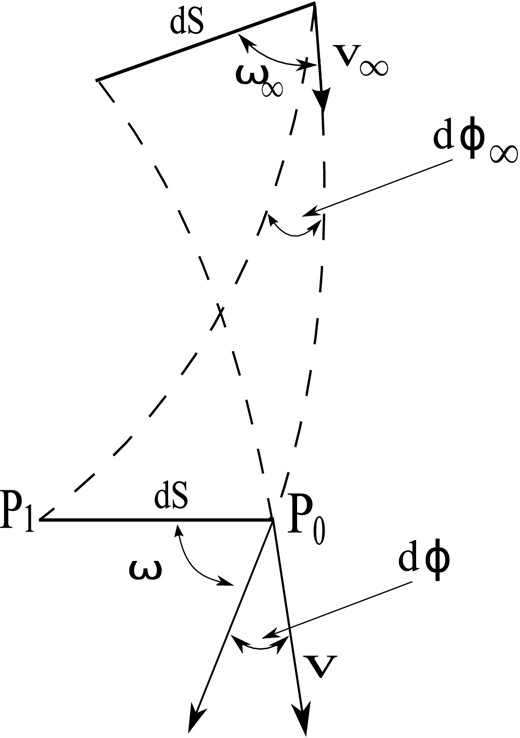
Schematic representation of orbits of field stars arriving to the cloud from infinity. The figure illustrates the fact that the number of stars in a given volume element in phase space is constant, which allows us to infer the field-star velocity distribution in the cloud from the field-star velocity distribution at infinity.
2.3 Criterion of capture
Our rule to decide whether a star is captured by the cloud is that the star position and velocity at the end of phase A, and hence its initial conditions for phase B, determine that the star orbits during the phase B period within the physical limits of the cloud (i.e. r ≤ a). This criterion excludes those stars that, even gravitationally captured (i.e. v < vesc), have orbits reaching the outer of the spheroid. However, this rather restrictive criterion simplifies greatly our calculations.
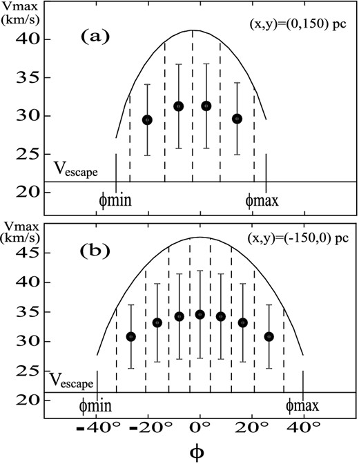
Diagrams showing the velocity directions (ϕ) and velocity magnitudes (v) of the stars that are located at the initial position (x, y) on the cloud and that will be captured. The escape velocity from the position (x, y) on the cloud, with the cloud at rest, is indicated. The field stars within the space ϕ–v enclosed by the curve vmax(ϕ) and the line indicating the escape velocity will be captured. The points and error bars show the mean velocities and velocity dispersions of the stars to be captured. The upper diagram corresponds to the position (x, y) = (0, 150) pc and the lower one to the position (x, y) = (− 150, 0) pc.
Therefore, in the phase space volume represented by each slab there is a star whose probable velocity is represented by the mean velocity and velocity dispersion of the corresponding slab (see Figs 2a and b), where the mean velocities and dispersions are indicated. In the examples of Figs 2(a) and (b), there are four stars (≈ ξN⋆*dV*P(r)) and seven stars, respectively, that can be captured. For the volume element of the examples given in Fig. 2, we have taken dV = 50 pc × 50 pc × 50 pc. In order to obtain the distribution of initial velocities and positions, on the whole cloud, of the finally captured stars, we divide the inner equatorial plane of the cloud into cells of area Δx × Δy = 50 pc × 50 pc and adopt, for each cell (or volume element), a height of 50 pc, perpendicular to the x–y plane. Fig. 3(a) displays the initial mean velocities in the corresponding central directions (ϕc) of the captured stars, obtained by means of the above explained method. Here, we have taken the central position of each cell as the initial positions of the stars contained in the cell. Fig. 3(a) shows that the captured stars have initial velocities in directions close to the positive x-axis, direction in which the cloud is accelerated. From equation (19), we calculate the distribution of the percentage of capture as a function of the initial positions of the finally captured stars (Fig. 3b). The stars located, at the beginning of phase A, at the rear of the cloud are captured in greater numbers. If the cloud is decelerated in phase A, the just mentioned distributions are given by the mirror images of Figs 3(a) and (b). We have used the following set of values for the model parameters, namely |$(a,e,\rho _{0}^{\rm A},\lambda ^{\rm A}, \alpha ^{\rm A}, t_{\rm f}^{\rm A})\!=\!(300\, \mathrm{pc}, 0.866, 7 \,\mathrm{at{\rm oms}\ cm}^{-3}, \frac{1}{10} \, \mathrm{Myr}^{-1}, -3.0\, \rm {km\, s^{-1}}\,{Myr^{-1}},$| 10 Myr). In the next section, we will give some justifications on the use of these particular values for the parameters of the model.
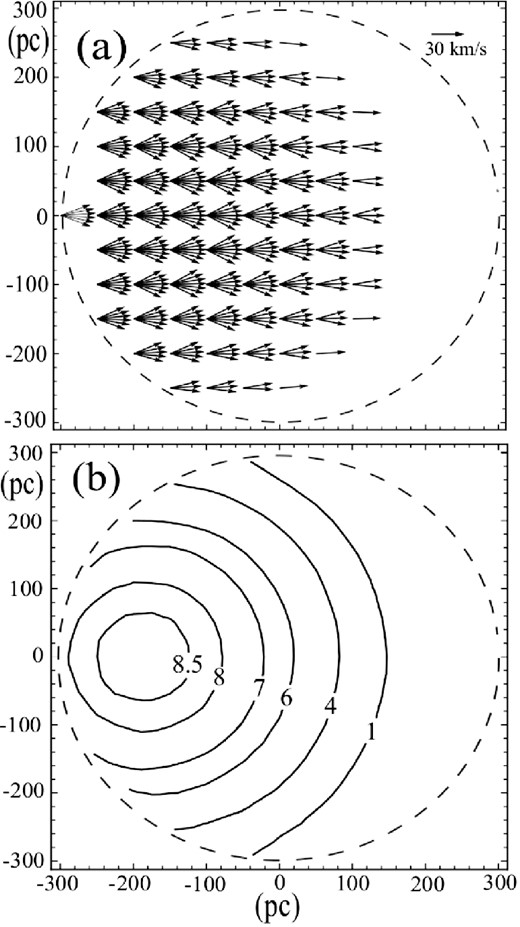
Panel (a) shows the initial mean velocities of the stars that will be captured for each volume element of 50 pc × 50 pc × 50 pc of the cloud's equatorial plane. The broken lines indicate the edge of the cloud. The velocity scale is given by the arrow (=30 km s−1) near the top-right corner. Panel (b) shows the initial spatial distribution of percentages of the stars that will be captured at the end of the first phase (phase A). The broken line indicates the edge of the cloud.
3 RESULTS
This model certainly permits the use of different values for the main parameters, as for instance the cloud dimension given by the semi-axis a and the eccentricity e or the cloud acceleration contained in the parameter α. In the next subsection, we will study the effects of varying the parameters within their physical limits. However, we require a priori that the cloud volume, |$\Omega =\frac{4}{3} \pi a^{2}\, b$|, be equal to the volume of a cylinder given by πa2H, where b is the semiminor axis of the spheroid and H the thickness of the H i Galactic layer ( ≈ 200 pc). Hence, |$b= \frac{3}{4} H$|. Since |$b= \sqrt{1-e^{2}}$|, |$e=\sqrt{1-(\frac{3 H}{4 a})^{2}}$|. Then, the value of e depends on the value adopted for a. On the other hand, we consider that the protocloud is dynamically stable and in consequence has a minimum density ρ0 = ρ⋆, where the so-called critical density |$\rho ^{\star }=\frac{0.165}{\beta _{1}} ({\mathrm{M}_{{\odot }}}\,{{\rm pc}^{-3}})=\frac{6.6}{\beta _{1}} ({\mathrm{atoms}}\,{\mathrm{cm}^{-3}})$| and β1 is a pure number that depends on |$\frac{b}{a}=\frac{3 H}{4 a}$| (see table 12⋆ of Chandrasekhar 1942).
We think of the interstellar cloud of this model as the progenitor of a gas–star complex. Elmegreen & Elmegreen (1983) found interstellar clouds with dimensions as large as 1 kpc and suggested that these superclouds may originate giant star complexes. The gas–star complexes have typical sizes of ≈650 pc (Alfaro, Cabrera-Cano & Delgado 1992a,b; Efremov 1995, 2010). In accordance with these facts, we adopt a = 300 pc and in consequence e = 0.866 and |${ \rho _{0}^{\rm A}=\rho ^{\star }=\,\, 7\,\mathrm{ atoms\, cm}^{-3}}$|.
3.1 Mean percentage of capture as a function of the parameters of the model
The distribution of the percentages of capture is not uniform over the cloud. This has a maximum at the back side of the cloud. In the example of Fig. 3(b), the maximum percentage of capture is ≈9 per cent, while the mean percentage is ≈4 per cent, averaged over the whole cloud. In other words, |$\overline{P}=\frac{\int ^{\Omega }P(r) {\rm d}V}{\int ^{\Omega } {\rm d}V}$|, where P(r) is given by equation (19). In this subsection, we characterize each chosen set of parameters of the model by its resulting mean percentage of capture.
We denote the parameter α, which corresponds to the cloud acceleration (with the sign minus), by αA during the phase A. Then, we can write αA in terms of the velocity of the cloud |$V_{\rm f}^{\rm A}$|, reached at the end of phase A |$(t=t_{\rm f}^{\rm A})$| as |$\alpha ^{\rm A} =-\frac{V_{\rm f}^{\rm A}-V_{0}^{\rm A}}{t_{\rm f}^{\rm A}}$|, where the initial velocity |$V_{0}^{\rm A}=0$|. From equation (1), the mass accretion rate of phase A, λA, can be expressed in terms of the final density |$\rho _{\rm f}^{\rm A}$| of this phase as |$\lambda ^{\rm A} = \frac{\rho _{\rm f}^{\rm A}-\rho _{0}^{\rm A}}{\rho _{0}^{\rm A}} \frac{1}{t_{\rm f}^{\rm A}}$|. That is to say that the set of parameters of phase A, namely (|$\alpha ^{\rm A}, \lambda ^{\rm A}, t_{\rm f}^{\rm A}$|) is equivalent to the set (|$V_{\rm f}^{\rm A},\rho _{\rm f}^{\rm A}, t_{\rm f}^{\rm A}$|). Setting |$V_{\rm f}^{\rm A}$| to a certain value, we can represent the mean percentage of capture as a function of |$t_{\rm f}^{\rm A}$|, |$\overline{P}(t_{\rm f}^{\rm A})$|, for different values of |$\rho _{\rm f}^{\rm A}$| (see Fig. 4).
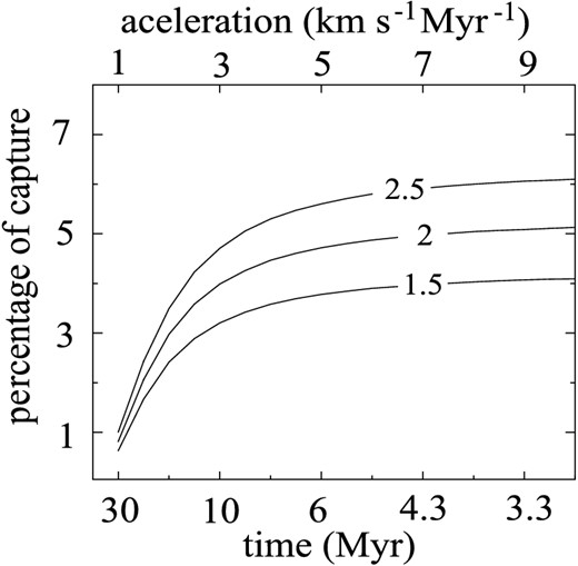
The mean percentage of captured field stars as a function of the duration of phase A (|$t_{\rm f}^{\rm A}$|) for the final densities of the cloud at the end of this phase |$\rho _{\rm f}^{\rm A}=1.5,\, 2$| and 2.5 times the initial density |$\rho _{0}^{\rm A} (=\rho ^{\star } = 7 \, \mathrm{atoms\,cm}^{-3})$|. The final velocity of the cloud at the end of this phase is fixed at |$V_{\rm f}^{\rm A}=30\,\mathrm{km\, s}^{-1}$|, velocity gained by the cloud during phase A due to a constant acceleration. The upper abscissa shows the corresponding accelerations.
Similarly, fixing |$\rho _{\rm f}^{\rm A}$| to a certain value, we can represent |$\overline{P}(V_{\rm f}^{\rm A})$|, for different values of |$t_{\rm f}^{\rm A}$| (see Fig. 5).
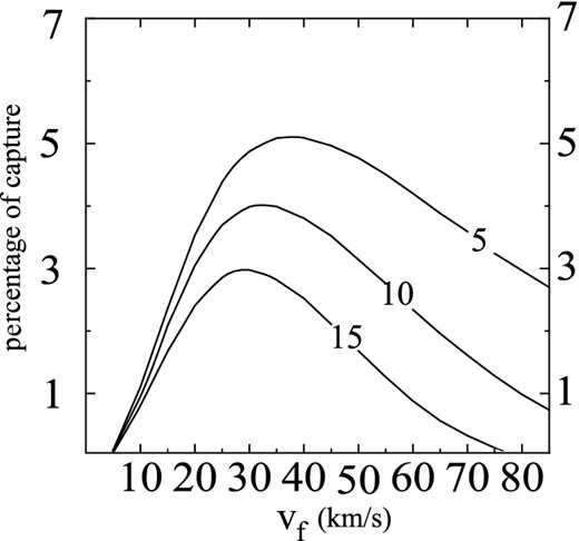
The mean percentage of captured field stars as a function of the final velocity |$V_{\rm f}^{\rm A}$| of the cloud at the end of phase A for different durations of phase A: |$t_{\rm f}^{\rm A}= 5,\,10$| and 15 Myr. The final densities of the cloud at the end of this phase is fixed at |$\rho _{\rm f}^{\rm A}= 2 \rho ^{\star }$| (i.e. two times the initial density |$\rho _{0}^{\rm A}$|), where ρ⋆ = 7 atoms cm−3.
The curves displayed by Fig. 4 show that the lower the time of acceleration the greater the percentage of capture. Also an increase of |$\rho _{\rm f}^{\rm A}$| implies an increase of |$\overline{P}(t_{\rm f}^{\rm A})$|. We adopt |${ \rho _{\rm f}^{\rm A}=2 \rho _{0}^{\rm A}= 2 \rho ^{\star }}$|, as a moderate value. Thus, the total mass of the cloud at the end of phase A is ≈2 × 10⁷ M⊙, which is within the range of the supercloud masses (Elmegreen & Elmegreen 1983). Besides, note that these curves have a turnover point at |$t_{\rm f}^{\rm A} \approx 10\,\mathrm{Myr}$|, from which the slope chances abruptly. Fig. 5 shows that the maximum of the percentage of capture occurs at |$V_{\rm f}^{\rm A} \approx 30{\rm -}40\,\mathrm{km\, s}^{-1}$|, which agrees approximately with the velocity dispersion of field stars, σ.
We will adopt |$t_{\rm f}^{\rm A}=10\, \mathrm{Myr}$|, although we have not a strong observational or physical justification, except that this time coincides roughly with the time needed for interstellar clouds to cross a spiral arm. We will adopt |$V_{\rm f}^{\rm A}=30\,\mathrm{km\, s}^{-1}$|, which is compatible with the velocity change experienced by gas clouds during the passage through an spiral arm (Roberts 1969, 1970). Hence, we adopt from now on (|$V_{\rm f}^{\rm A}, t_{\rm f}^{\rm A}, \rho _{\rm f}^{\rm A})=(30\,\mathrm{km\, s}^{-1}, 10\,\mathrm{Myr}, { 2 \rho ^{\star }})$|.
We have above assumed that the cloud's volume is constant. This consequently implies that the increment of the cloud's density should be entirely due to mass accretion, process in which the density would increase exponentially with time. However, we have adopted a linear law of density increment (equation 1). In the appendix, we demonstrate that the use of an exponential law for the cloud density variation, ρ(t) = ρ0eμt with μ = constant, yields results that are almost coincident with those we have obtained using equation (1).
Our model can too consider the case in which the cloud's density increment during phase A is purely due to a homologous contraction of the cloud. We assume that the cloud contracts from the initial semimajor axis a0 to the final one af. We here analyse the capture of the field stars lying at t = 0 within the cloud's inner volume delimited by the surface of an ellipsoid of semimajor axis af (i.e. within the final volume that the cloud reaches at the end of the contraction phase). The escape velocity vesc, used to determine the initial velocity distribution of the star field, must be calculated with a = a0 and the capture criterion with a = af. Since the cloud's mass |$M=\frac{4\pi \rho (t) a^{3}}{3}\sqrt{1-e^{2}}$| is here constant and if the density distribution remains homogeneous during the cloud's contraction, |$a_{0}=a_{\rm f} (1+ \lambda ^{\rm A} t^{\rm A}_{\rm f})^{\frac{1}{3} }= (\frac{\rho _{\rm f}^{\rm A}}{\rho _{0}^{\rm A}})^{\frac{1}{3}} a_{\rm f}$|. If af = 300 pc as adopted above for the size of the stable cloud and |$\frac{\rho _{\rm f}^{\rm A}}{\rho _{0}^{\rm A}}=2$|, we obtain a0 = 380 pc and the corresponding capture percentages shown in Fig. 6 by full lines. We have adopted the critical density ρ⋆ as the initial density of the cloud (i.e. |$\rho _{0}^{\rm A}= \rho ^{\star }$|). However, the model admits that the initial density can be lower. The model only requires that the density of the cloud at the end of phase A (|$\rho _{\rm f}^{\rm A}$|) must be greater than the critical density ρ⋆. For instance, if |$\rho _{0}^{\rm A}$| = |$\frac{1}{2} \rho ^{\star }$| and |$\rho _{\rm f}^{\rm A} =4 \rho _{0}^{\rm A}=2 \rho ^{\star }$|, we obtain a0 = 480 pc and the corresponding capture percentages shown in Fig. 6 by broken lines. Note that these results of Fig. 6 are only slightly lower than those of Fig. 5.
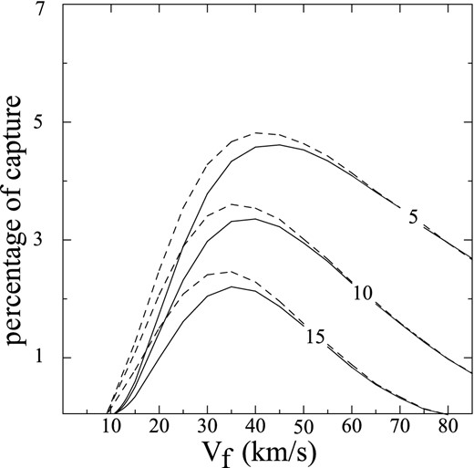
The same as Fig. 5, but calculated under the interpretation that the cloud's density increment is due to a process of compression and gravitational contraction. The broken-line curves represent the results obtained with the cloud initial density |$= \frac{1}{2} \rho ^{\star }$|, and the full-line curves those obtained with the cloud initial density =ρ⋆. In both cases, the final density is the same and equals 2ρ⋆.
Detailed studies of the formation and evolution of an interstellar gas cloud requires the realization of complex hydrodynamical calculations with the inclusion of gravitational and magnetic forces, shock waves, heating and cooling processes, turbulent motions, the cloud's rotation etc., which is out of the scope of this work. Nevertheless, we have shown above that the overall results on the capture of field stars are rather insensitive to the evolutionary details of the cloud.
3.2 Spatial distribution of positions and velocities of the captured field stars at the beginning and end of phases A and B
In this and the following sections, we consider that a and e remain constant during the three phases. Table 1 summarizes the values of the different parameters used in the simulations of each phase. In Section 2.3, we have defined the conditions of capture. For each considered volume element dV of the cloud, we make calculations similar to those represented in Figs 2(a) and (b). These figures delimit each initial velocity space that permits the capture of a star, and give the corresponding mean velocity |$\overline{v}$| and dispersion σ⋆ that characterize the probable initial velocity of the star. In the following simulations, the initial velocity v of the captured star and the angle ϕ (equation 18) are given by a number at random between |$\overline{v}-\sigma ^{\star }$| and |$\overline{v}+\sigma ^{\star }$| and between |$\phi _{\rm c}-\frac{{\rm d}\phi }{2}$| and |$\phi _{\rm c}+\frac{{\rm d}\phi }{2}$|, respectively. dϕ is the width of the corresponding vertical strip between the lines |$\phi = \phi _{\rm c}-\frac{{\rm d}\phi }{2}$| and |$\phi = \phi _{\rm c}+\frac{{\rm d}\phi }{2}$|, indicated by broken lines in the examples of Figs 2(a) and (b). For the position |$x_{0}^{\rm A},y_{0}^{\rm A}$|, we choose a number at random between |$x_{0}^{\rm A}-\frac{\sqrt[3]{{\rm d}V}}{2}$| and |$x_{0}^{\rm A}+\frac{\sqrt[3]{{\rm d}V}}{2}$|, and between |$y_{0}^{\rm A}-\frac{\sqrt[3]{{\rm d}V}}{2}$| and |$y_{0}^{\rm A}+\frac{\sqrt[3]{{\rm d}V}}{2}$|. Fig. 7(a) displays the initial positions and velocities of the star to be captured.
Panel (a): spatial distribution and velocity field at the start of the first phase (phase A) for the field stars that will be captured at the end of phase A. The arrows trace the velocity field of these stars. The velocity scale is given by the arrow (=30 km s−1) near the top-right corner. The broken lines indicate the edge of the cloud. Panel (b): spatial distribution and velocity field of the captured stars at the end of phase A.
Synopsis of the main parameters of the model. The semimajor axis a and the eccentricity e of the cloud are considered constant in the three phases and equal to 300 pc and 0.866, respectively.
| Phase A | Phase B | Phase C | ||||||||
|---|---|---|---|---|---|---|---|---|---|---|
| Parameter | Units | symbol | Value | symbol | Value | symbol | Value | Value | ||
| case (1) | case (2) | |||||||||
| Duration | Myr | |$t_{\rm f}^{\rm A}$| | 10 | |$t_{\rm f}^{\rm B}$| | undetermined | |$t_{\rm f}^{\rm C}$| | 10 | 10 | ||
| of the phase | ||||||||||
| Cloud's velocity | km s−1 | |$V_{0}^{\rm A}$| | 0 | |$V_{0}^{\rm B}$| | 30 | |$V_{0}^{\rm C}$| | 30 | 30 | ||
| at the phase's start | ||||||||||
| Cloud's velocity | km s−1 | |$V_{\rm f}^{\rm A}$| | 30 | |$V_{\rm f}^{\rm B}$| | 30 | |$V_{\rm f}^{\rm C}$| | 0 | 30 | ||
| at the phase's end | ||||||||||
| Acceleration of the cloud | km s− 1 Myr− 1 | −αA | 3.0 | −αB | 0 | −αC | −3.0 | 0 | ||
| |$= \frac{V_{\rm f}^{\rm A}-V_{0}^{\rm A}}{t_{\rm f}^{\rm A}}$| | |$= \frac{V_{\rm f}^{\rm C}-V_{0}^{\rm C}}{t_{\rm f}^{\rm C}}$| | |||||||||
| Cloud's density | atoms cm−3 | |$\rho _{0}^{\rm A}$| | 7 | |$\rho _{0}^{\rm B}$| | 14 | |$\rho _{0}^{\rm C}$| | 14 | 14 | ||
| at the phase's start | ||||||||||
| Cloud's density | atoms cm−3 | |$\rho _{\rm f}^{\rm A}$| | 14 | |$\rho _{\rm f}^{\rm B}$| | 14 | |$\rho _{\rm f}^{\rm C}$| | 0 | 0 | ||
| at the phase's end | ||||||||||
| Growth rate of the cloud's density | Myr−1 | λA | 0.1 | λB | 0 | λC | −0.1 | −0.1 | ||
| |$= \frac{\rho _{\rm f}^{\rm A}-\rho _{0}^{\rm A}}{\rho _{0}^{\rm A}} \frac{1}{t_{\rm f}^{\rm A}}$| | |$= \frac{\rho _{\rm f}^{\rm C}-\rho _{0}^{\rm C}}{\rho _{0}^{\rm C}} \frac{1}{t_{\rm f}^{\rm C}}$| |
Remembering that |$\alpha ^{\rm A} =-\frac{V_{\rm f}^{\rm A}-V_{0}^{\rm A}}{t_{\rm f}^{\rm A}}$| and |$\lambda ^{\rm A} = \frac{\rho _{\rm f}^{\rm A}-\rho _{0}^{\rm A}}{\rho _{0}^{\rm A}} \frac{1}{t_{\rm f}^{\rm A}}$|, and that we have adopted (|$V_{\rm f}^{\rm A}, t_{\rm f}^{\rm A}, \rho _{\rm f}^{\rm A})=(30\,\mathrm{km\, s}^{-1}, 10\,\mathrm{Myr}, 2 \rho _{0}^{\rm A})$|, we have the numerical values for all parameters and initial conditions needed to apply equations (8)–(11). Thus, we obtain the positions and velocities of the captured field stars at the end of phase A (Fig. 7b). The distributions represented by Figs 7(a) and (b) correspond to stars captured within the cloud's equatorial disc of thickness ΔH ( = 50 pc). In our model, the spatial and velocity distributions of the captured stars in the cloud's layers of different heights z are all equal. Hence, to obtain the total number of stars captured by the cloud, this relative number of captured stars (=362) should be multiplied by |$f_{\star } \frac{H}{\Delta H} \approx 160$|.
In order to calculate the star orbits in phase B by means of equations (12), we should take into account the continuity conditions prescribing that |$x_{0}^{\rm B}= x_{\rm f}^{\rm A}$|, |$y_{0}^{\rm B}= y_{\rm f}^{\rm A}$|, |$v_{0x}^{\rm B}= v_{{\rm f}x}^{\rm A}$|, |$v_{0y}^{\rm B}= v_{{\rm f}y}^{\rm A}$|, |$\rho _{0}^{\rm B}= \rho _{\rm f}^{\rm A}$|. Since the orbits are periodic in phase B, it not necessary to define the absolute duration of phase B; only the fraction of the orbit period T|$(=\frac{2 \pi }{k^{\rm B}} \approx 94\,{\rm Myr})$| in which the phase finishes. We give four possibilities for the relative durations of the phase, namely |$t_{\rm f}^{\rm B}(i)= i \frac{T}{4}+ n T$|, where i = 0, 1, 2 and 3, and n = 0, 1, 2, … We leave n undefined. The position and velocity distribution corresponding to |$t_{\rm f}^{\rm B}(0)$| agrees with the one at the end of phase A (Fig. 7b).
3.3 Space distribution of positions and velocities of the captured field stars at the end of phase C
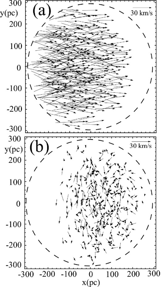
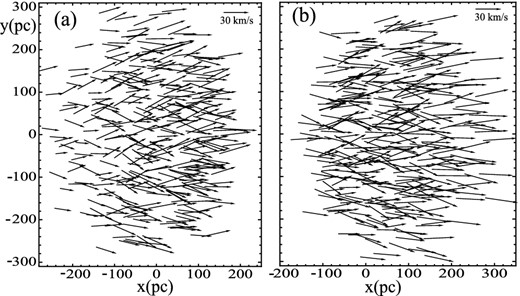
A summary of the parameter values used in this section is given in last columns of Table 1. Since the density of the cloud does not change during phase B, |$\rho _{0}^{\rm C}= \rho _{\rm f}^{\rm A}$|. Using also the final star positions and velocities of phase B as the initial conditions of phase C, we can apply equations (8)–(11) to calculate the star orbits in the phase under consideration. We take conveniently |$t_{\rm f}^{\rm C}=10\, \mathrm{Myr}$|, for the duration of phase C; with which the star orbits remain within the cloud borders where our equations are valid. We consider two possibilities for the development of phase C that lead to similar results: (1) the cloud is decelerated (or accelerated, if it has been decelerated during phase A) and loses all its mass; (2) the cloud loses all its mass, but here the velocity of the cloud as a whole is unaffected. Therefore for case (1), we have that |$\alpha ^{\rm C} =-\frac{V_{\rm f}^{\rm C}-V_{0}^{\rm C}}{t_{\rm f}^{\rm C}}$| and |$\lambda ^{\rm C} = \frac{\rho _{\rm f}^{\rm C}-\rho _{0}^{\rm C}}{\rho _{0}^{\rm C}} \frac{1}{t_{\rm f}^{\rm C}}$|, where |$\rho _{\rm f}^{\rm C}=0$| and |$V_{0}^{\rm C}=V_{\rm f}^{\rm A}$|. If |$V_{\rm f}^{\rm C}=0$|, the cloud in its last stage of disintegration is at rest in the adopted inertial system of coordinates. Hence, the star velocities given by equations (10) and (11) at the end of phase C coincide with the star velocities referred to the inertial system, which could be assimilated to the LSR. Then |$\alpha ^{\rm C} =-\frac{-V_{\rm f}^{\rm A}}{t_{\rm f}^{\rm C}}$|, |$\lambda ^{\rm C} = -\frac{1}{t_{\rm f}^{\rm C}}$| and uC = 0. Substituting u = uC = 0 and |$u_{0}=u_{0}^{\rm C}$| into the last two terms of equations (8) and (10), we find that |$-\frac{\pi \alpha }{( u_{0} \lambda )^{2} }\, Ai(u) \int _{ u_{0}}^{u}\, Bi(u) {\rm d}u + \frac{\pi \alpha }{(u_{0} \lambda )^{2} }\, Bi(u) \int _{ u_{0}}^{u}\, Ai(u) {\rm d}u =\frac{1}{2} \frac{ \alpha ^{\rm C}}{(\lambda ^{\rm C})^{2}}=\frac{1}{2} V_{\rm f}^{\rm A} t_{\rm f}^{\rm C}$| and that |$-\frac{\pi \alpha }{ u_{0} \lambda } \dot{Ai}(u) \int _{ u_{0}}^{u} Bi(u) {\rm d}u + \frac{\pi \alpha }{ u_{0} \lambda } \dot{Bi}(u) \int _{ u_{0}}^{u} Ai(u) {\rm d}u= -\frac{ \alpha ^{\rm C}}{\lambda ^{\rm C}}=V_{\rm f}^{\rm A}$|. Thus, the x-component of the position and of the velocity in case (1) can be written |$x_{\rm f}^{\rm C}(1)= \chi (1)+\frac{1}{2} V_{\rm f}^{\rm A} t_{\rm f}^{\rm C}$| and |$v_{{\rm f}x}^{\rm C}(1)=\nu (1)+ V_{\rm f}^{\rm A}$|, where χ(1) and ν(1) represent the first two terms of equations (8) and (10), respectively. Since αC = 0 in case (2), the two last terms of equations (8) and (10) are null and therefore |$x_{\rm f}^{\rm C}(2)= \chi (2)$| and |$v_{{\rm f}x}^{\rm C}(2)=\nu (2)$|. In order to refer the velocity |$v_{{\rm f}x}^{\rm C}(2)$| to the inertial system, the velocity |$V_{\rm f}^{\rm C}= V_{\rm f}^{\rm A}$| should be added to |$v_{{\rm f}x}^{\rm C}(2)$|. For a given star χ(1) = χ(2) and ν(1) = ν(2), hence the final velocity in x agrees in both cases and the x-component of the position differs only in a constant. On the other hand, |$y_{\rm f}^{\rm C}(1)= y_{\rm f}^{\rm C}(2)$| and |$v_{{\rm f}y}^{\rm C}(1)=v_{{\rm f}y}^{\rm C}(2)$|. In other words, cases (1) and (2) are equivalent. The distribution of positions and velocities of the captured stars at the final of phase C depends on the adopted |$t_{\rm f}^{\rm B}(i)$| (see Section 3.2). Figs 8(a) and (b) show the final star positions and velocities of phase C derived with |$t_{\rm f}^{\rm B}(0)$| and with |$t_{\rm f}^{\rm B}(2)$|, respectively. The velocity distribution corresponding to Fig. 8(a) (with plus symbols) and to that of Fig. 8(b) (with point symbols) are shown in Fig. 9.
Spatial distributions and velocity fields for the captured field stars at the end of the final phase (phase C). The positions, magnitudes and directions of the vectors indicate the positions and velocities of the stars. We here draw a representative fraction of the total number of captured stars, which multiplied by a factor of ≈160 gives the total number of captured stars. The distributions are obtained with the duration of phase B given by |$t_{\rm f}^{\rm B}(0)$| (panel a), and by |$t_{\rm f}^{\rm B}(2)$| (panel b).

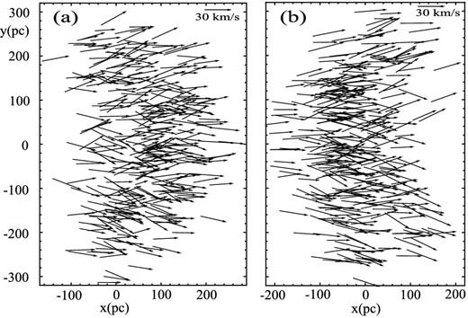
Figs 10(a) and (b) show the final star positions and velocities of phase C derived with |$t_{\rm f}^{\rm B}(1)$| and with |$t_{\rm f}^{\rm B}(3)$|, respectively. The velocity distribution corresponding to Fig. 10(a) (with plus symbols) and to that of Fig. 10(b) (with point symbols) are shown in Fig. 11.
Spatial distributions and velocity fields for the captured field stars at the end of the final phase (phase C). The positions, magnitudes and directions of the vectors indicate the positions and velocities of the stars. We here draw a representative fraction of the total number of captured stars, which multiplied by a factor of ≈160 gives the total number of captured stars. The distributions are obtained with the duration of phase B given by |$t_{\rm f}^{\rm B}(1)$| (panel a), and by |$t_{\rm f}^{\rm B}(3)$| (panel b).

3.4 The capture of the Sun
A question that we should answer is whether the Sun's position among the local moving groups is by chance or not. There is a fact that might indicate that it is not by chance. The Sun's velocity with respect to the LSR is much lower than the velocity dispersion of the G-type stars. This could indicate that the Sun has interacted with an interstellar cloud. This possibility is of great interest because of its possible effects on the Earth's environment (Clube & Napier 1986; Bailey, Clube & Napier 1990).
So the relatively low LSR-velocity of the Sun could be explained by means of a mechanism of capture. The Sun met an interstellar cloud in coincidence with the passage of a spiral arm that decelerated suddenly the cloud. Another possibility is that the collision of an HVC with the Galactic disc accelerated a concentration of Galactic gas, through which the Sun was circumstantially passing. In the course of the last 400 Myr, a flow of HVCs coming from the Magellanic Clouds might have collided with the gas layer of the Galactic disc (Olano 2004). We propose that the same cloud that captured the Sun captured the field stars of the local moving groups.
Figs (8)–(11) represent the distributions of positions and velocities for the captured field stars of all spectral types, at the end of phase C. Here our aim is to analyse these distributions only for the captured field stars of solar type (i.e. G-type stars). Since the field stars of solar type have ages of 5 Gyr and velocity dispersions ≥35 km s−1 (Nordström et al. 2004), following the method of Section 2.3, we use the lower limit of integration given by |$v_{G}=\sqrt{v_{\infty }-2\Phi (r)}$|, where v∞ = 35 km s−1. Note that when v∞ = 0, vG = vesc (see equation 19), and that the ϕ range of integration depends too on the value of vG (see Fig. 2). In order to derive the distribution of positions and velocities for this particular type of stars, we use |$t_{\rm f}^{\rm B}(i)$| of phase B, where i=0, 1, 2 and 3, and case (2) of phase C. For the rest of the parameters, we use the same values as before, except for N⋆, where we use N⋆ = 0.02 stars pc−3 (i.e. we should multiply by a factor f⋆ = 4 to obtain the star density observed in the solar vicinity). The resulting distributions are displayed in Figs 12 and 13. Since the LSR velocity of the Sun is ≈15 ± 5 km s−1, the velocity components of the captured stars with kinematics similar to that of the Sun at the present should lie between the circle of radius of 10 km s−1 and that of 20 km s−1. Note that only the velocity distributions of the cases |$t_{\rm f}^{\rm B}(1)$| and |$t_{\rm f}^{\rm B}(2)$| contain stars with velocities within the mentioned velocity interval.
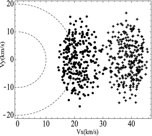
Distribution of velocity components for the captured field stars of solar type at the end of the final phase. The plus symbols correspond to the case |$t_{\rm f}^{\rm B}(0)$| and the point symbols to the case |$t_{\rm f}^{\rm B}(2)$|. The region between the two concentric circles traced by broken lines corresponds to the velocity range in which the LSR solar velocity lies.

The same as Fig. 12 but for the case |$t_{\rm f}^{\rm B}(1)$| (plus symbols) and for the case |$t_{\rm f}^{\rm B}(3)$| (point symbols).
The total velocities of the same stars, when they were outside the gravitational influence of the perturbing cloud, were of the order of 40 km s−1. That is to say that the interaction with the perturbing cloud could reduce the velocities of this star group from 40 to only 15 km s−1. The distributions of Figs 12 and 13 correspond to the cloud's equatorial disc of thickness ΔH ( = 50 pc). Since the number of stars between the concentric circles is ≈100 (89 for the case |$t_{\rm f}^{\rm B}(2)$| and 139 for the case |$t_{\rm f}^{\rm B}(1)$|), the density of G stars with solar kinematics is |$\frac{100 f_{\star }}{ \pi a^{2} \Delta H} \approx 3\, \times 10^{-5}$| stars pc−3. Then the number of G stars with solar kinematics in the whole volume of the cloud (|$\frac{4}{3} \pi a^{3} \sqrt{1-e^{2}}$|) is ≈2 × 10³ stars. Certainly, these numbers depends on the values adopted for the parameters, in particular for |$V_{\rm f}^{\rm A}$|. However, they show the explaining capacity of the model. Therefore, the results of the our simulations support the hypothesis delineated above.
3.5 Stellar stream formed by stars born in the giant interstellar cloud
In addition to a collector of field stars, the giant interstellar cloud is thought to be a site of star formation. We assume that the new stars are formed during phase B. The disintegration of the cloud, considered in phase C of the model, may be attributed in part to the activity of the stars born in the cloud.
Let us present a simple simulation of phases B and C for the stars born in the cloud. We divide the equatorial disc of the cloud into cells of volume dV(ΔxΔyΔH = 50 pc × 50 pc × 50 pc). We consider that the gas of any element dV is in a circular orbit in the x–y plane and gives origin to the formation of a star. The circular orbit of a gas element dV of initial position (r, θ) is obtained from equations (12) with the initial conditions given by x0 = r cos θ, y0 = rsin θ, v0x = −vccos (π/2 − θ), v0y = vcsin (π/2 − θ), where vc = kB r. Thus, the gas cells rotate in the equatorial plane of the cloud as a rigid body with the angular rotation velocity |$\frac{v_{\rm c}}{r}= k_{B}$|. For the initial conditions of the newborn star, we take random numbers in the ranges (x0 − δx0, x0 + δx0) and (y0 − δy0, y0 + δy0), for the position, and (v0x − δv0x, v0x + δv0x) and (v0y − δv0y, v0y + δv0y), for the velocity. We adopt δx0 = δy0 = 25 pc and δv0x = δv0y = 5 km s−1. The number of stars (|$=\frac{\pi a^{2} \Delta H }{{\rm d}V}$|) adopted for the simulations is certainly arbitrary; and the adoption of uniform number density of stars is not realistic. However, these simulations of illustrative character would permit us to infer the results that the use of more realistic conditions should produce.
We assume that the stars were born at the same time throughout cloud and have an age, at the end of phase B, between 0 and |$t_{\rm f}^{\rm B}(i)$| (|$= i \frac{T}{4}+ n T$|, see Section 3.3). Since the absolute values of |$t_{\rm f}^{\rm B}(i)$| are not necessary for our purposes, we can adopt a fraction of the period as the age of the stars. Since the results obtained using different fractions of the period are very similar, we will take as representative the case i = 0. The position and velocity distributions at the end of phase C resulting from our simulation are shown in Figs 14 and 15. The stars born in a certain region of the cloud during a short time interval share close positions in the position and velocity distributions at the end of phase C. Hence, an enhancement of the star formation activity in a relatively small region of the cloud is reflected in the position and velocity distributions as a compact moving group.
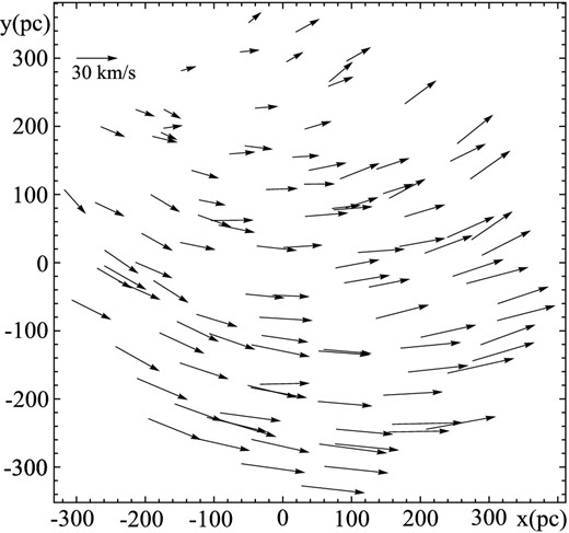
Spatial distribution and velocity field, at the end of the final phase (phase C), for the stars born in the cloud.
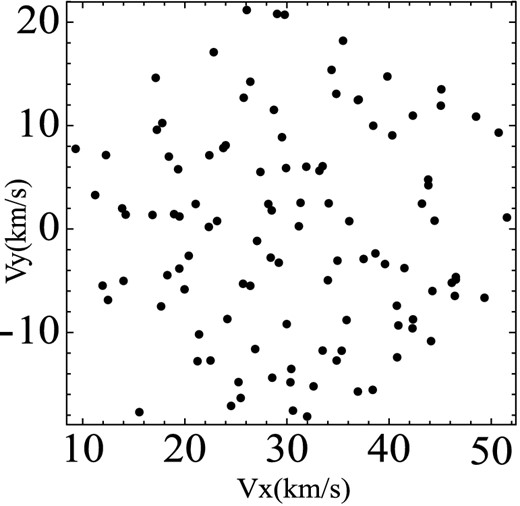
Distribution of velocity components corresponding to the velocity field of Fig. 14.
4 CONCLUSIONS
In the light of our model, giant star–gas complexes of the Galaxy that probably suffered strong accelerations in their genesis would contain an important component of captured field stars. The giant star–gas complexes have typical sizes of ≈650 pc (Alfaro et al. 1992a,b; Efremov 1995, 2010), and in agreement with this, the semimajor axis of the model's cloud is 300 pc. The model's mechanism produces a kinematic selection of the field stars within the cloud, because only the stars with initial velocities close to the direction of the cloud's acceleration are captured. The maximum percentage of capture is obtained with an acceleration that, acting during 10 Myr, produces a cloud's peculiar velocity of ≈30 km s−1. Our model shows that, averaged over the whole cloud, an ∼4 per cent of the field stars contained in the original cloud's volume are captured by the interstellar cloud. The subsequent disruption of the cloud's gaseous mass in the last evolutionary stages leaves the stars as moving groups. Therefore, the model can explain the presence of age-homogeneous moving groups as well as of age-heterogeneous ones within the same star complex.
There are two mechanisms that could accumulate interstellar material of a vast region and simultaneously accelerate (or decelerate) it to form a self-gravitating interstellar cloud accelerated or decelerated with respect to the passing field stars. First, according to the classical theory of spiral density waves, a gaseous cloud that enters into a density wave is decelerated and compressed in the associated shock wave. Since the velocity dispersion of the gas is much smaller than that of the stars, the response of the gas to the density waves would be much stronger. This effect could produce a relative deceleration between gas and field stars. However, we should mention that recent simulations of the dynamics of stars and gas around spiral arms show complex results (Baba et al. 2009; Wada, Baba & Saitoh 2011; Grand, Kawata & Croper 2012). From the observational side, direct determinations of distances and proper motions of star-forming regions in spiral arms of our Galaxy with interferometer techniques of very long baseline (Reid et al. 2009 and references therein) show that there are star–gas complexes with peculiar velocities as large as 30 km s−1. Secondly, the Milky Way is immersed in a stream of HVCs coming from the Magellanic Clouds. Therefore, these HVCs have been hitting the Galactic disc during a large period of time, and one of the consequences would be the formation of the Galactic warp (Olano 2004; Bobyley 2010; Abedi et al. 2014). The fall of an HVC on the gaseous layer of the Galactic disc can transfer momentum to the gas contained in a large volume without affecting the field stars of the region.
The main aim of the work has been to study the proposed capture mechanism with reasonable astrophysical parameters. The chosen model parameters of 300 pc for the semimajor axis of the cloud and of 14 atoms cm− 3 for the cloud's maximum density, corresponding to the cloud's mass of 2 × 10⁷ M⊙, are representative of the sizes and masses of the giant star–gas complexes (Elmegreen & Elmegreen 1983). The velocity of 30 km s−1 adopted for the cloud's peculiar velocity due to the acceleration process is approximately the velocity with which the cloud captures the maximum percentage of stars (see Figs 5 and 6). Furthermore, the corresponding velocity distributions (see Figs 9, 11 and 15) cover velocity ranges similar to those of the velocity distribution of single stars of the local moving groups. Indeed, the mean space velocity (|$=\sqrt{\overline{U}^{2}+\overline{V}^{2}}$|) and the velocity dispersion of the local system of moving groups are ≈25 and ≈± 15 km s−1, respectively (see fig. 2 of Montes et al. 2001). The election of the parameter's value for the duration of the acceleration process is, however, more uncertain because of our ignorance of the mechanisms and circumstances involved in the cloud's acceleration (or deceleration). We have adopted a duration of 10 Myr for the acceleration phase, but a difference of ±5 Myr with respect to the adopted time implies a difference of ∓1 in the capture percentages (see Figs 5 and 6).
Our model is intended as a first step in this line of study of the stellar moving groups. A detailed comparison with the observational data should require to extend this model into a more complex one. This new model should consider that the cloud is in a Galactic orbit and that the motions of the stars associated with the cloud are also affected by the general gravitational field of the Galaxy. In this treatment, the motion equations referred to the cloud's gravity centre contain terms due to the Coriolis force. This force plays an important role, together with the rotation sense of the supercloud, in shaping the moving-group velocity distributions and their vertex deviations (Olano 2001; Bobyley 2004). Then, the values of the model's free parameters can be obtained by fitting the simulation results to the observational data of the moving groups. Another limitation of the model is that we use a rather restrictive criterion of capture, considering as captured only the stars whose orbits remain within the physical contour of the cloud. On the other hand, the approximation of representing the cloud as a homogeneous ellipsoid facilitates the analytic solution, but the real clouds have irregular forms and inhomogeneous mass distributions. The formation and evolution of giant cloud complexes are not well known and the involved physical processes are very complex (e.g. Elmegreen 1979, 1987, 1992). Further theoretical and observational developments in this research field will help to do more realistic simulations of the star capture processes
Finally, we propose that the moving groups of the solar neighbourhood have a common origin in the way considered by our model. The existence of kinematic substructures that characterize the different moving groups would reflex irregularities in the initial spatial distribution of the number density of stars. The model supports also the possibility that the Sun was captured by the same gas–star complex that would have given origin to the moving groups of the solar neighbourhood, and more recently to Gould's belt (Olano 2001). This possibility is of great interest for the studies of natural history of the Earth. Encounters of the Solar system with substructures of the giant cloud could have perturbed recurrently the Oort cometary cloud, causing rains of comets on the Earth (Clube & Napier 1986; Bailey et al. 1990).
ACKNOWLEDGEMENT
I was benefited from the comments of an anonymous referee.
Member of The Carrera del Investigador Científico, CONICET, Argentina.
REFERENCES
APPENDIX A: SOLUTION OF THE MOTION EQUATIONS
- (a) The case of a linear time variation of the supercloud's density: ρ(t) = ρ0(1 + λt). The x-motion equation (6) is a non-homogeneous equation and in order to obtain its solution, we should first solve the associated homogeneous equationThe change of variable u = u0(1 + λt), where |$u_{0}=-(\frac{k}{ \lambda })^{2/3}$|, transforms equation (A1) into an Airy equation: |$\ddot{x}(u)-u x(u)=0$|. The solution of the Airy equation is of the form x(t) = c1x1(t) + c2x2(t), where x1(t) and x2(t) are given by the Airy functions of first kind, Ai(u), and of second kind, Bi(u), respectively, and the quantities c1 and c2 are constants. The general solution of equation (6) can be expressed in terms of the solution of equation (A1) and of one particular solution xp(t) of the nonhomogeneous equation (6) as follows:(A1)\begin{equation} \ddot{x}+k^{2} (1+ \lambda t) x=0. \end{equation}The solution xp(t) can be obtained by means of the method of variation of parameters. Thus, proposing that(A2)\begin{equation} x(t) =c_{1} x_{1}(t) +c_{2} x_2(t)+ x_{p}(t). \end{equation}and imposing arbitrarily the condition |$\dot{c_{1}}(t) x_{1}(t)+\dot{c_{2}}(t)x_{2}(t)=0$|, we can find the functions c1(t) and c2(t) that allow xp(t) to be one solution of the non-homogeneous equation. These functions are |$c_{1}(t)=-\int \frac{f(t) x_{2}(t)}{W(t)}{\rm d}t$| and |$c_{2}(t)=\int \frac{f(t) x_{1}(t)}{W(t)}{\rm d}t$|, where in our case f(t) = α = constant and |$W(t)=x_{1}(t) \dot{x_{2}}(t)-\dot{x_{1}}(t) x_{2}(t)$|, the so-called Wronskian determinant. Thus, |$W(t)=W \lbrace Ai(u), Bi(u)\rbrace \dot{u}$|, where W{Ai(u), Bi(u)} = π−1 (Abramowitz & Stegun 1964). Therefore, |$c_{1}(t)=-\frac{\pi \alpha }{u_{0} \lambda } \int _{0}^{t} Bi(u){\rm d}t=-\frac{\pi \alpha }{(u_{0} \lambda )^{2}} \int _{u_{0}}^{u_{0} (1+\lambda ) t} Bi(u){\rm d}u$|, and |$c_{2}(t)= \frac{\pi \alpha }{u_{0} \lambda } \int _{0}^{t} Ai(u){\rm d}t= \frac{\pi \alpha }{(u_{0} \lambda )^{2}} \int _{u_{0}}^{u_{0}(1+\lambda t)} Ai(u){\rm d}u$|. Remembering that x1(t) = Ai(u) and x2(t) = Bi(u), and making the corresponding replacements in equation (A3), we obtain(A3)\begin{equation} x_{p}(t)= c_{1}(t) x_{1}(t)+c_{2}(t)x_{2}(t), \end{equation}The constants c1 and c2 in equation (A2) are determined from the initial conditions. At t = 0, xp(0) = 0, x1(0) = Ai(u0), x2(t) = Bi(u0), |$\dot{x_{1}}(0)= \dot{Ai}(u_{0}) u_{0} \lambda$|, and |$\dot{x_2}(0)= \dot{Bi}(u_{0}) u_{0} \lambda$|. The dot over the Airy functions denotes the derivative with respect to u. Hence, x0 = x(0) = c1Ai(u0) + c2Bi(u0) and |$v_{0x}=\dot{x}(0)= c_{1} \dot{Ai}(u_{0}) u_{0} \lambda +c_{2} \dot{Bi}(u_{0}) u_{0} \lambda$|. Solving this system of two equations for c1 and c2, we obtain(A4)\begin{eqnarray} x_{p}(t)&=&-\frac{\pi \alpha }{(u_{0} \lambda )^{2}} Ai(u) \int _{u_{0}}^{u_{0}(1+\lambda ) t} Bi(u){\rm d}u \nonumber \\ &&+\frac{\pi \alpha }{(u_{0} \lambda )^{2}} Bi(u)\int _{u_{0}}^{u_{0} (1+\lambda t)} Ai(u){\rm d}u. \end{eqnarray}Substituting equations (A5) and (A4) into (A2), we have the general solution given by equation (8). The solution of the y-motion equation (7) is analogous to that of equation (A1).(A5)\begin{eqnarray} c_{1} &=& \pi x_{0} \dot{Bi}(u_{0})- \frac{\pi v_{0x}}{ u_{0} \lambda } Bi(u_{0}), \nonumber \\ c_{2} &=& -\pi x_{0} \dot{Ai}(u_{0})+ \frac{\pi v_{0x}}{ u_{0} \lambda } Ai(u_{0}). \end{eqnarray}
- (b) The case of an exponential time variation of the supercloud's density: ρ(t) = ρ0eμt, where ρ0 and μ are constants. By similarity with the x-motion equation (6), we haveThe transformation |$u=\frac{2 k}{\mu } {\rm e}^{ \mu t}$| converts the homogeneous equation associated with equation (A6) into |$\ddot{x}(u)+\frac{1}{u}\dot{x}(u)+ x(u)=0$|, the Bessel differential equation of order zero. Its solution is given by x(u) = c1J0(u) + c2Y0(u), where c1 and c2 are arbitrary constants, and J0(u), Y0(u) are the so-called Bessel functions of order zero, of the first and second kinds, respectively. If the particular solution of the non-homogeneous equation (A6) is of the form |$x_{p}(t)= c_{1}(t) J_{0}(\frac{2 k}{\mid \mu \mid } {\rm e}^{ \mu t}) +c_{2}(t) Y_{0}(\frac{2 k}{\mid \mu \mid } {\rm e}^{ \mu t})$|, we obtain by means of the method of variation of parameters |$c_{1}(t)=-\int \frac{\alpha Y_{0}(\frac{2 k}{\mid \mu \mid } {\rm e}^{ \mu t})}{W(t)}{\rm d}t$| and |$c_{2}(t)=\int \frac{\alpha J_{0}(\frac{2 k}{\mid \mu \mid } {\rm e}^{ \mu t})}{W(t)}{\rm d}t$|, where |$W(t)=W \lbrace J_{0}(u), Y_{0}(u)\rbrace \dot{u}=\frac{\mu }{\pi }$| and |$\dot{u}=k {\rm e}^{\frac{\mu t}{2}}$|. Therefore, the general solution of equation (A6) is(A6)\begin{equation} \ddot{x}+k^{2} {\rm e}^{ \mu t} x=\alpha . \end{equation}where |$u=\frac{2 k}{\mid \mu \mid }$|. Hence, the velocity is given by(A7)\begin{eqnarray} x(t)&=& c_{1} J_{0}(u)+c_{2} Y_{0}(u)-\frac{\alpha \pi }{\mu } J_{0}(u) \nonumber \\ &&\times\,\int _{0}^{t} Y_{0}(u){\rm d}t + \frac{\alpha \pi }{\mu }Y_{0}(u) \int _{0}^{t} J_{0}(u){\rm d}t, \end{eqnarray}The dot over the Bessel functions denotes the derivative with respect to the variable u. From equations (A7) and (A8) with t = 0, and having into account that |$\dot{J}_{0}(u)=-J_{1}(u)$| and |$\dot{Y}_{0}(u)=-Y_{1}(u)$| (Abramowitz & Stegun 1964), we obtain a system of two equations relating the initial conditions with the constants c1 and c2, namely x0 = x(0) = c1J0(u0) + c2Y0(u0) and |$v_{0x}=\dot{x}(0)=- k c_{1}J_{1}(u_{0})- k c_{1}Y_{1}(u_{0})$|, where |$u_{0}=\frac{2 k }{\mid \mu \mid }$|. Solving this equation system for c1 and c2 and replacing the values of these constants in equation (A7), we obtain(A8)\begin{eqnarray} \dot{x}(t)&=&c_{1} \dot{J}_{0}(u)\dot{u}+c_{2} \dot{Y}_{0}(u)\dot{u}\nonumber \\ &&-\frac{\alpha \pi }{\mu } \dot{J}_{0}(u)\dot{u} \int _{0}^{t} Y_{0}(u){\rm d}t + \frac{\alpha \pi }{\mu }\dot{Y}_{0}(u)\dot{u} \int _{0}^{t} J_{0}(u){\rm d}t. \end{eqnarray}and by similarity(A9)\begin{eqnarray} x(t)&=& \frac{k \pi }{\mu } (J_{1}(u_{0}) Y_{0}(u)-J_{0}(u) Y_{1}(u_{0}))\, x_{0}\nonumber \\ &&- \frac{ \pi }{\mu } (J_{0}(u) Y_{0}(u_{0})-J_{0}(u_{0}) Y_{0}(u))\, v_{0x} \nonumber \\ &&- \frac{\alpha \pi }{\mu } J_{0}(u) \int _{0}^{t} Y_{0}(u){\rm d}t + \frac{\alpha \pi }{\mu }Y_{0}(u) \int _{0}^{t} J_{0}(u){\rm d}t, \end{eqnarray}(A10)\begin{eqnarray} y(t)&=& \frac{k \pi }{\mu } (J_{1}(u_{0}) Y_{0}(u)-J_{0}(u) Y_{1}(u_{0}))\, y_{0}\nonumber \\ &&- \frac{ \pi }{\mu } (J_{0}(u) Y_{0}(u_{0})-J_{0}(u_{0}) Y_{0}(u))\, v_{0y}. \end{eqnarray}
(c) Comparison of the results obtained from both cases: we have calculated λ from the initial and final density of the cloud in the considered phase (see Table 1). Similarly we obtain that |$\mu =\frac{\ln (\frac{\rho _{{\rm f}}}{\rho _{0}})}{t_{{\rm f}}}$|. Comparing equations (8) and (A9) and, equations (9) and (A10), we note that the values of respective coefficients of the initial conditions and of the respective independent terms are very similar for any fixed value of the parameters. Therefore, the results obtained for both cases are almost coincident.
