


Abstract
We use about 15 000 F/G nearby dwarf stars selected from the LAMOST pilot survey to map the U–V velocity distribution in the solar neighbourhood. An extreme deconvolution algorithm is applied to reconstruct an empirical multi-Gaussian model. In addition to the well-known substructures, e.g. Sirius, Coma Berenices, Hyades–Pleiades overdensities, several new substructures are unveiled. A ripple-like structure from (U, V) = (−120, −5) to (103, −32) km s−1 is clearly seen in the U–V distribution. This structure seems associated with resonance induced by the Galactic bar, since it is extended in U while having a small dispersion in V at the same time. A ridge structure between (U, V) = (−60, 40) and (−15, 15) km s−1 is also found. Although similar substructures have been seen in the Hipparcos data, their origin is still unclear. Another compact overdensity is seen at (U, V) = (−102, −24). With this large data sample, we find that the substructure located at V ∼ −70 km s−1 and the Arcturus group are essentially parallel in V, which may indicate that they originate from an unrelaxed disc component perturbed by the rotating bar.
1 INTRODUCTION
The origin of the substructures in the velocity distribution in the solar neighbourhood is not clear, although several theories have been proposed. For a long time, it was believed that the substructures are associated with disrupted stellar clusters (Kapteyn 1905; Eggen 1965; Skuljan, Cottrell & Hearnshaw 1997; etc.), which is probably where the name stellar moving groups comes from. When Hipparcos (Perryman et al. 1997) data became available, with accurate parallaxes and proper motions for tens of thousands nearby stars, Dehnen (1998) recognized that the moving groups follow the asymmetric drift relation, i.e. older groups are hotter and on eccentric orbits, which seems associated with resonance induced by non-axisymmetric force. Famaey et al. (2005, 2007), Famaey, Siebert & Jorissen (2008) found that the member stars of some moving groups have a wide range of age, mass, and metallicity, which does not imply a disrupted cluster origin. Bensby et al. (2007) also claimed that the Hercules stream has a range of age and chemical abundances. These observations indicate that stellar cluster disruptions are not responsible for most of the well-known substructures, e.g. the Sirius, Hyades, Pleiades, Hercules streams, but may be for a few moving groups, e.g. HD 1614 (De Silva et al. 2007). Consequently, theoretical works tend to explain the moving groups as the dynamical effects of the bar and/or spiral arms of the Milky Way.
Weinberg (1994) showed that the Galactic bar can lead to distinctive stellar kinematics near the Outer Lindblad resonance (hereafter OLR). Dehnen (2000), who analysed the properties of several types of the closed stellar orbits near to the OLR using test particle simulations, concluded that the unstable |$x_{1}^{*}(2)$| orbits produce the valley between the Hercules substructure and the majority of the stars in the U–V distribution, where U is the radial velocity (U > 0 towards the Galactic Centre) and V is the tangential velocity. In his model, there are a few elongated features, one of which, located at U > 0, V < 0, is caused by stars on nearly closed orbits with large perturbative amplitudes around the OLR. Moreover, he reproduced ripple-like feature associated with the outer 1:1 resonance in his simulation. Variations in the U–V distribution associated with the angle of the bar, the strength of the bar, the OLR location, and the shape of the rotation curve were also constrained in his work. Fux (2001), on the other hand, focused more on the orbital analysis and split the stellar orbits into regular, which belong to the disc, and chaotic, which are migrated from the region within the co-rotation radius of the bar. As a consequence, he inferred that the Hercules overdensity is due to the outward mixed stars on chaotic orbits. In his test particle simulation, resonances generate distinct arcs in the velocity plane, which open towards lower angular momentum. Unlike Dehnen (2000), the 1:1 resonance plays no role in the Fux model. On the contrary, the 4:1 resonance feature, which consists of x1(2) orbits, can be recognized, particularly for cases with R/ROLR < 1 (inside the OLR). Note that there are no substructures corresponding to the cold moving groups, e.g. Sirius, Hyades, Pleiades, etc. in both the Dehnen (2001) and Fux (2001) simulations. These smaller scale substructures are more likely related to the local spiral arm(s) (Antoja et al. 2011; Quillen et al. 2011).
With only data from the solar neighbourhood, the origin of the velocity substructures may not be constrained well. Since simulations can easily predict the velocity distribution at different positions in the Galactic disc (Dehnen 2000; Fux 2001; Bovy, Hogg & Roweis 2009; etc.), stellar kinematics beyond the solar neighbourhood are required and will play an important role in this study. Recently, Antoja et al. (2012) used RAVE data to map the velocity distribution at about 1 kpc around the Sun and found that the Hercules overdensity is a decreasing function of the Galactocentric radius. Based on a test particles simulation similar to Dehnen (2000), Antoja et al. (2013) inferred that this is induced by the rotating Galactic bar. Liu et al. (2012) also found that the radial velocity of red clump stars shows a bifurcation at 10–11 kpc in Galactocentric radius in the Galactic anticentre direction, which may again be associated with the bar.
The ongoing LAMOST survey (Zhao et al. 2012) will observe several million dwarf stars in low resolution, and will provide the largest spectroscopic sample within a few kpc around the Sun (Deng et al. 2012). This data set will provide the velocity distribution at different positions in the azimuth-radius plane, and thus will enable the investigation of the role of resonances induced by the rotating bar in the velocity distribution.
The LAMOST pilot survey has publicly released in excess of 600 000 stellar spectra. We select more than 14 000 F and G dwarf stars from the pilot survey and map them on to the U–V plane. In this paper, we show new evidence, within 500 pc around the Sun, associated with resonances of the Galactic bar. The structure of the paper is as follows. In Section 2, we outline the extreme deconvolution method developed by Bovy et al. (2009), which we apply to derive the intrinsic distribution of the LAMOST stars in the U–V plane. We validate the method using mock data with various velocity errors to help identify the detection limits of the substructure scale. In Section 3, we introduce how the stars are selected and their distances estimated. The selection bias of the data is taken into account and corrected using photometric data. In Section 4, we show the resulting U–V distribution for the whole data set and for subsamples inside and outside the solar circle (R0 ≃ 8 kpc). In Section 5, we discuss the new features revealed in the U–V distribution and give possible explanations for their existence. We conclude our investigation in Section 6.
2 EXTREME DECONVOLUTION
We derive the intrinsic distribution of the LAMOST stars in the U–V plane using the extreme deconvolution method described in Bovy et al. (2009). In this section, we summarize the key points of the deconvolution method relevant to our investigation.
In principle, the velocity error may affect the performance of the extreme deconvolution. Small and fine structures in the velocity distribution may not be recovered by the extreme deconvolution if the error of the observed velocity is too large. In theory, structures with scale smaller than the error are unreliable. So we set the regularization parameter w (Bovy et al. 2009) roughly the same as the square of the error. We perform Monte Carlo simulations to investigate this effect.
We select 10 Gaussians as the original distribution using the parameters listed in table 1 of Bovy et al. (2009). Because only U and V are considered in our work, the dimension W (vertical velocity) of these Gaussians is ignored. The true U–V distribution of the 10-Gaussian model is shown in Fig. 1(a). The scales 1 of the components vary from 2.3 to 95 km s−1. Notice that the scales of the three compact Gaussian components located between U ∼ −50 and 0 km s−1 at V ∼ −20 km s−1 are 5.6, 9.3, and 4.7 km s−1, respectively, from the left to right. The scales of the Gaussians at (U, V) ∼ (−22, −10) km s−1 and (9, 4) km s−1 are 17 and 10 km s−1, respectively. To create the data, we randomly generate 20 002 mock stars from the original 10-Gaussian distribution, and with additional arbitrary Gaussian errors as the test data. The U–V distribution is reconstructed using a 12-Gaussian empirical model with the extreme deconvolution method. Figs 1(b), (c), and (d) show the results with the Gaussian errors at 3, 8, and 12 km s−1, respectively. The corresponding regularization parameters w are chosen to be 9, 64, and 144 km2 s−2. As mentioned before, we set w comparable with the velocity uncertainties of the data. If w is set with a value smaller than the velocity uncertainty, smaller structures can be revealed, however, they are usually spurious. On the other hand, larger structures should not be affected by the smoothing, provided that the value of w is not too large. Therefore, we select w to be comparable to the velocity uncertainty squared.
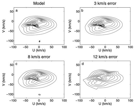
The mock U–V velocity distribution. The contours contain, from inside outward, 1, 3, 8, 13, 25, 40, 48, 65, 75, 83, 89, and 94 per cent of stars.
For the test with a random error of 3 km s−1, Fig. 1(b) shows that almost all of the substructures in the original distribution are reconstructed, except the low-amplitude one at (0, −100) km s−1. The random initial conditions of the extreme deconvolution and relatively fewer Gaussian components may lead to the loss of small substructures. For the test with random error of 8 km s−1, Fig. 1(c) shows that the three most compact structures around V ∼ −20 are not distinguishable and turn into a single larger scale substructure. When the measurement error goes up to 12 km s−1, the component at (−22, −10) km s−1, together with the three most compact substructures, is merged into a single larger substructure centred around (−25, −15) km s−1. The larger component at (9, 4) km s−1 is still distinguishable, but an elongated Gaussian component is added to connect it with other substructures, making an artificial ridge from (−80, −30) to (50, 15) km s−1. For the test case of the 10-Gaussian U–V distribution, which mimics the true distribution in the solar neighbourhood, when the measurement error of the velocity is as high as 12 km s−1, the extreme deconvolution cannot properly recover smaller scale substructures while some artefacts may also affect the larger scale components in terms of their shapes.
3 OBSERVATIONAL DATA
The proper motions of the sample are obtained by cross-identifying with the PPMXL catalogue (Röeser, Demleitner & Schilbach 2010). It is noted that the systematic bias of the proper motions in PPMXL is not negligible (Wu, Ma & Zhou 2011). Therefore, we use QSOs (quasi-stellar object) to correct the bias on a star-by-star basis (see Appendix for details).
3.1 Distance estimation
The distance of the F/G dwarf stars in the sample can be estimated from the colour index and metallicity. Fig. 2 shows the absolute magnitude, MK, as a function of (J − K)0 and [Fe/H] in the isochrones given that log (age/yr) = 7.85 (Girardi et al. 2002). We use the relatively young isochrones here because they cover the full range of the colour index (J − K)0. However, this may induce a systematic bias in the distance estimation. In principle, the young population should be a little fainter than an old one on the main sequence. This may lead to an underestimation of the distance by a factor of 20 per cent, which would produce an underestimate of U and V by a similar percentage. Since these systematics rescale U and V by similar factors for most of the stars, they will not significantly change the relative distribution of the stars in the U–V plane.
![The absolute magnitude in the K band, MK, as a function of (J − K)0 and [Fe/H]. The dots show the synthetic samples from isochrones with log (age/yr) = 7.85. The colour encodes the metallicity. The series of lines show the best surface plane fit for this relation.](https://oup.silverchair-cdn.com/oup/backfile/Content_public/Journal/mnras/447/3/10.1093_mnras_stu2620/2/m_stu2620fig2.jpeg?Expires=1749848507&Signature=nMBXKzxv-~T7PxtzZUXZ7nsPcPUTB0lvqF6boCytS5Z5gvbv-DQWDx~IgX6qcQZM3XVUaMlMCNNu6gEj6UkNdEoNvhz7nyxe1WbRr75KZkgThfgX50pd8~KQ6Cj5hl-JntgeyXNlrz7uL2SP7EWKium-e8AiCdrKA49Ow9hpRHg47TvP5NnrHBKk7UaYG7tm0aXDbBG1wFvD2YeZHTS--x6brWmxku4J5OwV-DRheLtLn-jykg11KzecAZk5QCKdmi9ZMtCPWarbXPD1nQWZeUdCvxZrpjbeV4-mzdeEtiyHbwyX0-Ud~WZLhQXKOOVKH0cq947bUN8ADDtZdZ4CCg__&Key-Pair-Id=APKAIE5G5CRDK6RD3PGA)
The absolute magnitude in the K band, MK, as a function of (J − K)0 and [Fe/H]. The dots show the synthetic samples from isochrones with log (age/yr) = 7.85. The colour encodes the metallicity. The series of lines show the best surface plane fit for this relation.
The LAMOST pilot survey does not provide [Fe/H], and hence we can only obtain the probability density function (PDF) of MK for a star given a metallicity distribution function (MDF) in the solar neighbourhood. Hou et al. (1998, see also the top panel of Fig. 3) provide an MDF for G dwarf stars in the solar neighbourhood, which is suitable for our sample. Although the MDF may shift to the metal-poor end with increasing height (z) over the Galactic mid-plane, it can only introduce at most a 4 per cent difference in the distance estimation at z = 0.5 kpc given that the vertical metallicity gradient is −0.3 dex kpc−1. This subsequently leads to at most a 2 km s−1 shift in the tangential velocity (V) when the true velocity is 50 km s−1. Therefore, we simply assume the MDF is constant with z in this paper. The PDFs of distance for three sample stars are shown in the right-hand panel of Fig. 3.
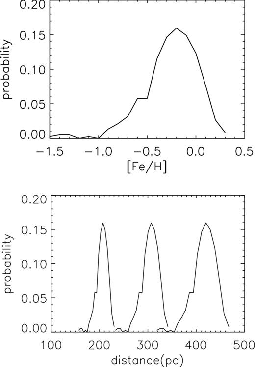
Top panel: the MDF for G dwarf stars in the solar neighbourhood (Hou, Chang & Fu 1998). Bottom panel: the PDFs of distance for three samples of F/G dwarf stars at various distances. The PDFs are derived from the MDF shown in the top panel.
Fig. 4 shows the 3D positions in heliocentric Cartesian coordinates for the 14 662 selected F/G dwarf stars based on their mean distance estimates. We select stars between 100 and 500 pc in z for two reasons. First, stars located nearer than 100 pc are not completely sampled in the LAMOST pilot survey since they are too bright. This may lead to some strong selection effects. Secondly, the stars located farther away than 500 pc are dominated by luminous stars and thus lead to selection effects in the opposite way. Therefore, we select stars within this range to keep the luminosity function approximately constant at different z.
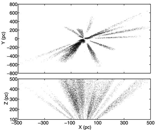
The locations, in the galactic coordinate system, of the stars we used. The direction of the positive x-axis is towards the Galactic Centre.
The velocity components U and V in heliocentric Cartesian coordinates are calculated according to Johnson & Soderblom (1987). Because the distance of a star in this work follows a certain PDF, the U and V are also random variables based on the distance PDF. Fig. 5 shows the distribution of the mean U and V derived from the mean distances. The Hercules stream, which leads to an obvious asymmetry in U is clearly displayed in the figure. More detailed substructures will be unveiled in Section 4 after applying the extreme deconvolution algorithm to the data.
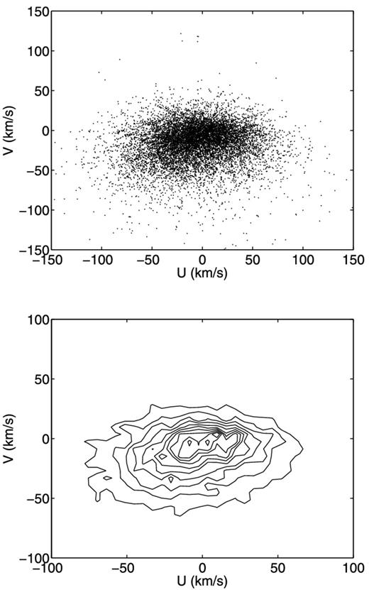
Top panel: scatter plot of the velocity distribution in the U–V plane. Bottom panel: the contour of the velocity distribution in the U–V plane. The contours contain, from inside outward, 3, 8, 19, 30, 39, 50, 59, 71, 85 per cent of stars.
3.2 Selection correction
In general, the sampling of a spectroscopic survey is significantly affected by the selection strategy, observational conditions, data reduction, etc. These may induce selection bias. In order to reduce the selection effects in the resulting U–V distribution, we use photometric data to correct the bias.
Fig. 6 shows the distribution of ϖ for the data set. The peak value of ϖ is around 2, meaning that each star in the spectroscopic samples represents usually two photometric ones with similar position, magnitude, and colour index. The stars with ϖ larger than 6 (about 20 per cent of the total number of stars) have been removed from our sample because they are highly undersampled and may not therefore represent the kinematic features for similar stars. Furthermore, stars with 0.5 ≤ ϖ < 1 are also excluded. They may either be observed more than once, or have a smaller value of Nsp due to very few stars counted in the given volume and hence are not suitable for later statistical studies.
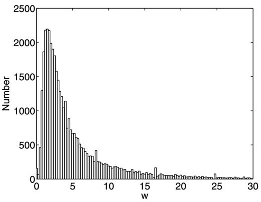
The histogram of the selection correction weights (see the text in Section 3.2). Particles with 0.5 ≤ ϖ ≤ 6 are used in our study.
4 RESULTS
4.1 Reconstruction of the intrinsic U–V distribution
In order to reconstruct the U–V distribution for the selected samples, Monte Carlo simulations combined with the extreme deconvolution are used. First, a random distance for each star is drawn from the distance PDF and then a pair of corresponding U and V is determined. Secondly, an extreme deconvolution with 20 Gaussians is applied to such a data set in the U–V plane. Comparing the model predicted radial velocities to those of the stars from the GCS catalogue, Bovy et al. (2009) inferred that 10 Gaussians can work well to reconstruct the U–V–W distribution with Hipparcos data. For our case, we use 20 Gaussians in our model in each random draw according to Appendix B. Since the velocity error is around 6 km s−1, the regularization parameter w in this fitting is chosen to be 36 km2 s−2.
We run 100 random draws and derive the median U–V distribution over the 100 20-Gaussian models. We compare the median U–V distribution to that averaged over the first 50 draws and find that the main structures do not significantly change. Therefore, we believe that the results from 100 draws have converged and hence are sufficient for the reconstruction of the U–V distribution.
We also run the extreme deconvolution with average distance to estimate the U–V distribution in order to save computational time (see Fig. 8). However, we argue below that the Monte Carlo simulations used here can lead to better resolution in the U–V distribution and therefore is able to reveal more detailed features than simply using the average distance.
First, the Monte Carlo simulations can take into account the non-Gaussian profile of the uncertainty in distance, while the extreme deconvolution with the average distance can only approximate it as a Gaussian and may miss some information due to the non-Gaussian profile. Secondly, the dispersion in U–V distribution due to the uncertainty in distance in the Monte Carlo simulations should be equivalent with that in the extreme deconvolution with average distance. However, because the uncertainty of the average distance is propagated to U and V, their uncertainties should be slightly larger than a single realization in the Monte Carlo process. The 10 per cent distance uncertainties generate additional 5 km s−1 velocity errors which increase the velocity errors from about 6to 8 km s−1 in both U and V. Therefore, we use a slightly larger regularization parameter, w = 64 (km s−1)2, in the extreme deconvolution with average distance than that in the Monte Carlo processes, for which we take w = 36 (km s−1)2. The larger regularization may lead to a slightly smoother distribution but smaller substructures will be blurred. Finally, in general, the true U–V distribution may contain more substructures than the Gaussian components of an empirical model. It implies that the extreme deconvolution with a limited number of Gaussians actually smoothens out the U–V distribution and may miss some subtle substructures due to the lack of Gaussian components to represent for them. However, in the Monte Carlo simulation, for each realization, we first apply 20 Gaussians in the empirical U–V distribution model and finally apply 100 × 20 after 100 simulations. Recall that the regularization parameter is smaller in the Monte Carlo simulations, which implies that it is more sensitive to smaller substructures than the extreme deconvolution method. Therefore, the Monte Carlo simulations not only have far more Gaussian components to represent the substructures, they also have an advantage in revealing smaller substructures. Although averaging the 100 × 20 Gaussians may eventually smooth out some substructures, nevertheless, the reproductions of small substructures in some realizations will still remain in the final distribution. We conclude that the Monte Carlo simulations (shown in Fig. 7) can reveal more details than the average distance approach in Fig. 8.

The figure shows the velocity distribution in the U–V plane. The contours contain, from inside outward, 2, 6, 12, 21, 32, 48, 58, 70, 81, 88, 94, and 97 per cent of stars. The circles are the central positions of the overdensities in RAVE (Antoja et al. 2012). The identified structures are marked as crosses or dashed lines with a number aside. The detailed locations and the names of the known substructures are listed in Table 1.
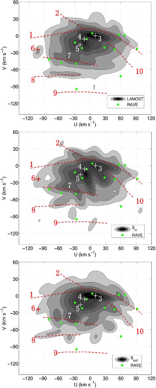
The top panel shows the U–V distribution using the mean distances. The middle panel is the velocity distribution of the Sin sample (for stars within the solar circle, R < R0) and the bottom panel is the velocity distribution of the Sout sample (for stars beyond the solar circle, R > R0). The contour levels are the same as in Fig. 7.
4.2 Known overdensities in the LAMOST data
Fig. 7 shows our results. Table 1 lists all the identified substructures in Fig. 7. Unlike the results based on the wavelet transform (e.g. Chereul, Crézé & Bienaym 1999; Zhao, Zhao & Chen 2009; Antoja et al. 2012; etc.), the LAMOST pilot survey data shows very smooth structures in the U–V distribution, except for the two compact overdensities in the core of the distribution, i.e. structures 3 and 4, which are the Sirius and Coma Berenices structures, respectively. The centre of the two overdensities is a few km s−1 offset from Antoja et al. (2012, shown as the circles in the figure). This is probably because the velocities between the RAVE and LAMOST data are not well calibrated, especially the contribution from the proper motions.
The list of substructures unveiled from Fig. 7.
| No. | Name | U range | V range |
|---|---|---|---|
| 1 | NEW | −120 to 103 | −5 to − 32 |
| 2 | NEW | −60 to − 15 | 40 to 15 |
| 3 | Sirius | 11 | −1 |
| 4 | Coma Berenices | −11 | −7 |
| 5 | Hyades–Pleiades | −18 | −18 |
| 6 | NEW | −102 | −24 |
| 7 | Hercules | −95 to 5 | −38 to − 50 |
| 8 | Arifyanto06 | −111 to − 14 | −73 to − 68 |
| 9 | Arcturus | −64 to 37 | −100 to − 102 |
| 10 | Wolf 630 | 33 to 90 | −11 to − 58 |
Note. Arifyanto06 – Found by Arifyanto and Fuchs (2006).
Hyades and Pleiades overdensities are connected with each other and marked as structure 5 in Fig. 7. The two overdensities may be parts of one single elongated substructure at V ∼ −20 km s−1. Indeed, Famaey et al. (2005) did not separate them using CORAVEL/Hipparcos/Tycho-2 data. They can be separated in studies based on the wavelet transform since it tends to remove the low-frequency (or smooth) components and enhance the high-frequency (or clumpy) components. On the other hand, it is unlikely that they are not distinguished by our extreme deconvolution method because of the uncertainty of the velocity. Dehnen (1998) found the central velocity of Hyades is at U = −40 km s−1 and that of Pleiades is at U = −25 km s−1. Antoja et al. (2012) measured the central values as −30 and −16 km s−1, respectively, in the U component with RAVE data. In any case, the two overdensities are separated by 15 km s−1, larger than the uncertainty of the velocity in this work by a factor of 2. The validation test discussed in Section 2 demonstrates that our method is capable of distinguishing substructures with such separation in the U–V distribution. Therefore, the merging of Hyades and Pleiades overdensities in the LAMOST pilot survey data may either be because of fluctuations within a larger substructure, or due to different sampling volumes with Hipparcos and RAVE.
Although the Hercules stream (structure 7) is also not separated from other structures, it shows a clear asymmetry in Fig. 7. Recall that we select only the F and G dwarf stars (relatively young) in our samples. The non-separation of the Hercules stream is consistent with Dehnen (1998), in which the author showed that the Hercules stream is not as prominent for stars with 0 < B − V < 0.6 than older stars with B − V > 0.6. This implies that it is composed of relatively old populations, although the age range may be very broad, according to Famaey et al. (2005). Compared with Antoja et al. (2012), which fixed the Hercules stream at V ∼ −50 km s−1, the LAMOST data has a slightly faster V velocity at about −40 km s−1.
Another hot overdensity is structure 8, which is located at V ∼ −70 km s−1 and extends by around 100 km s−1 in U. This is consistent with the overdensity discovered by Arifyanto & Fuchs (2006). Indeed, because the central position of the overdensity is around U ∼ 50 km s−1, we can obtain that |$\sqrt{U^2+2V^2}\sim 111$| km s−1, which is completely in agreement with their study.
The Arcturus group (Eggen 1971; marked as structure 9) is also seen at V ∼ −100 km s−1 close to the bottom of Fig. 7. Here, with a larger sample, we confirm that the Arcturus group is also elongated along U, consistent with groups 14, 17, and 19 in Antoja et al. (2012). The most overdense region of the elongated substructure is at U ∼ −25 km s−1, which overlaps well with their group 14.
Combining the images of the two elongated hot substructures at V ∼ −70 and −100 km s−1, it seems that they form a wave-like picture. Minchev et al. (2009) argued that such structures may arise from the unrelaxed disk ∼1.9 Gyr ago due to a perturbation caused by a recent merger event.
4.3 New substructures
A few new substructures are unveiled in the U–V distribution. The most obvious substructure is the thin ripple-like structure 1 at the top of the majority of the stars found in Fig. 7. Because we use multiple Gaussians to build the empirical model of the U–V distribution and a Gaussian profile cannot be made to form a ripple-like structure, the algorithm automatically selects two Gaussians with elongated covariance matrices to reconstruct such a substructure following the observed data. The substructure is also seen, somewhat blurred, in the top panel of Fig. 8 in which the PDF of the distance is replaced with the mean distance. This elongated feature is not prominent in other survey data, e.g. Hipparcos (Dehnen 1998; Bovy et al. 2009 etc.), GCS (Zhao et al. 2009), and RAVE (Antoja et al. 2012, 2013). This is probably due to two reasons. First, the Hipparcos and GCS only cover stars within 100 pc around the Sun, while the LAMOST pilot data can reach as far as 500 pc. Although the RAVE data can reach a similar depth, it covers only the Southern Galactic cap, and with only a small fraction of the sky overlapping with the LAMOST survey. Secondly, some previous works used the wavelet transform method, which concentrates more on the small scale overdensities, and thus probably filters out such larger scale features.
Structure 1 has a narrower dispersion in V with an extended dispersion in U, which leads to a significantly larger σU/σV (∼3, approximated from the ratio of the major- and minor-axis of the contours in Fig. 7) than that for the whole sample (<2). It cannot be explained by the population being kinematically hot, but may be associated with a resonance, which enhances only the radial excursion of the stellar orbits but not the azimuthal velocity. Meanwhile, the relatively higher V of the substructure indicates that many stars move faster than the local circular speed. Hence, their orbital guiding centre radii may be beyond the solar circle. In other words, this population should be from the outer disc. If the resonance is induced by the central rotating bar, then according to equations 3.150 and 3.80 in Binney & Tremaine (2008), the 1:1 OLR is indeed around R = 10.6 kpc if the circular speed is 220 km s−1 and the bar pattern speed is 50 km s−1 kpc−1. The complete orbital phases of stars experiencing the resonance of the Galactic bar should form a narrow annulus with somewhat large radius in the U–V plane. For the case of 1:1 OLR, the resonance radius should be beyond the solar orbit, and therefore, the 1:1 OLR stars observed in the solar neighbourhood are only samples with orbital phase close to the pericentre. This leads to an incomplete annulus at around the maximum of V in the U–V plane, similar to feature 1. However, the pattern speed can be as low as 40 km s−1 kpc−1 (Long et al. 2013) and the local circular speed as high as 250 km s−1 (Reid et al. 2009). Therefore, the position of the OLR is uncertain and the precise nature of the resonance is not conclusive. For instance, if we adopt the pattern speed of the bar inferred from Long et al. (2013), and the local circular speed of 220 km s−1, the 2:1 OLR is then at R = 9.4 kpc, which is more likely to be responsible for the ripple-like structure.
Just above structure 1, the new ridge-like structure 2 is located from (−15, 15) to (−60, 40) km s−1. A similar feature also appears in the GI bottom-left panel of fig. 3 in Dehnen (1998), in which a ridge-like structure with (U, V) from (−5, 10) to (−30, 40) km s−1 is indicated. The B2, B3, B4, and AL panels of fig. 3 of Dehnen (1998) also show some evidence of feature 2. It is not clear if this feature is an extension of the Sirius overdensity (labelled as 3 in Fig. 7) since they are apparently connected with each other. It seems that member stars moving out with higher speed (i.e. smaller negative U) have larger angular momenta (i.e. larger V).
Yet another new overdensity, structure 6, is found at (−102, −24) km s−1. It may be either a new feature or the tail of the Hercules stream containing a clump of stars moving outward.
5 THE U–V DISTRIBUTION AT DIFFERENT GALACTOCENTRIC RADII
The substructure induced by the resonance of the bar and spiral arms in the velocity distribution may vary with position. Dehnen (2000) mapped various simulated U–V distributions at different radii and azimuthal angles with respect to the central bar. With the RAVE data, Antoja et al. (2012, 2013) found that, indeed, the location of the Hercules stream and the gap between the Hercules stream and the majority of the stars varies with radius. The variation of the Hercules stream at different locations may well constrain the pattern speed and azimuthal angle of the Galactic bar. The volume of the LAMOST pilot data used in this work is similar to that of RAVE. Therefore, it is worth investigating the variation of the U–V distribution for stars inside of, and outside of the solar circle (R0 ≃ 8 kpc).
Although using the PDF of the distance with Monte Carlo simulation can gain a slightly better resolution of the substructures, it is very time consuming. Hence, we use the median distance estimated from the PDF of distance to map the U–V distribution for two subsamples with R < R0 and R > R0, respectively. In these fits, we use 31 Gaussians and the regularization parameter, w, is taken to be 64 km2 s−2.
We first verify if the median distance can give the same U–V distribution as that of the PDF of the distance. The top panel of Fig. 8 shows the U–V distribution for the whole sample with median distance. The substructures appear much broader than those in Fig. 7, because (1) there are far more Gaussians used in Fig. 7 than in the top panel of Fig. 8; and (2) since the uncertainties of U and V are slightly larger due to the additional contribution of the uncertainty in the distance, we set w = 64 km2 s−2 in Fig. 8. Even so, most of features except structure 9 are still recognizable. Therefore, we can use the median distance to map the U–V distribution for the stars located inside and outside the solar circle. The other panels of Fig. 8 show the two U–V distributions with R < R0 (middle panel) and R > R0 (bottom panel).
The Hyades–Plaiedes overdensity (structure 5) is still seen in the U–V distribution inside the solar circle but is no longer recognizable in the one outside the solar circle. This implies that most of its member stars are located inside the solar circle. Moreover, below the Hyades–Pleiades structure, there is an extended feature from (−10, −15) to (5, −50) km s−1 in the middle panel of Fig. 8. This feature can also be identified in the third column panel of fig. 3 of Antoja et al. (2012).
The Hercules stream (structure 7), on the other hand, is clearly separated from the majority of the stars in the U–V distribution outside the solar circle, but not separable in the U–V distribution inside the solar circle. This is in agreement with Antoja et al. (2012, 2013).
In the U–V distribution outside the solar circle, structure 10 (which should be the Wolf 630 overdensity according to Antoja et al. 2012) is clearly seen just below the Sirius overdensity, while it is not recognizable in the U–V distribution inside the solar circle. This is also approximately consistent with the RAVE results demonstrated by Antoja et al. (2012).
The ripple-like structure 1, which is prominent in Fig. 7, is no longer clearly seen in the U–V distribution neither inside nor outside the solar circle. However, structure 2 is even more prominent in the U–V distribution inside the solar circle.
It is not easy to find the origins of the variations of the substructures with Galactocentric radii. Quillen et al. (2011) showed a possible scenario from their N-body simulation where these subtle substructures may be associated with the relative locations of the spiral arms. Antoja et al. (2011) inferred that the inner Lindblad resonances induced by the spiral arms at different radii may also produce different patterns of substructures in the U–V distribution.
6 CONCLUSIONS
The goal of the LAMOST pilot survey is to verify the survey design and to test the performance of the instruments: it is not expected to be as good as the formal (ongoing) survey. Even so, the pilot survey has already collected sufficient data for an investigation of the local velocity distribution. Radial velocity estimation is sufficiently accurate to distinguish kinematic substructures with velocities around 6–10 km s−1. With these data, we are able to identify known and new substructures in the U–V velocity distribution. Three new substructures, 1, 2, and 6 (see Table 1 and Fig. 7), are found from the data. Structure 1 is likely associated with the resonance induced by the central Galactic bar. Structures 8 and 9 (Acturus group) are consistent with a scenario where the local disc is being perturbed by the Galactic bar according to Minchev et al. (2009).
When we separate the data into two samples at the solar circle, the U–V distributions of the two groups of stars are significantly different. The Hercules stream is more isolated in the sample beyond the solar circle, while the Hyades–Pleiades substructure is more prominent in the sample inside the solar circle. The latter could be associated with the spiral structures of the Milky Way, but it remains a puzzle how the spiral structures can produce such spatial variations. More data covering larger ranges of distances is required to constrain better the origin of these subtle substructures on nearly circular orbits. We plan to investigate these issues with the LAMOST DR1 data in a future study.
This work is supported by the National Science Foundation of China under grant no. 11373032, 11333003 (CL and SM), and 11390372 (SM). CL acknowledges the Major State Basic Research Development Programme 2014CB845704. This work has also been supported by the Strategic Priority Research Programme ‘The Emergence of Cosmological Structures’ of the Chinese Academy of Sciences Grant No. XDB09000000 (SM and CL). The Guoshoujing Telescope (the Large Sky Area Multi-Object Fiber Spectroscopic Telescope, LAMOST) is a National Major Scientific Project built by the Chinese Academy of Sciences. Funding for the project has been provided by the National Development and Reform Commission. LAMOST is operated and managed by the National Astronomical Observatories, Chinese Academy of Sciences. We thank the referee for his (or her) detailed comments that have helped improve this paper substantially.
LAMOST Fellow.
In this paper, the scale of a 2D Gaussian is defined as the square root of the trace of the covariance matrix.
REFERENCES
APPENDIX A: PROPER MOTION CORRECTION
The proper motions in the PPMXL catalogue (Röser et al. 2010) have apparent systematic errors which will affect the U–V velocity distributions. If we assume the systematic error is 1 mas yr− 1 and the distance to a star is 500 pc, the difference in U–V velocity plane will be about 2 km s−1. On the other hand, the mean errors of the proper motions in the PPMXL catalogue vary from 4 mas yr− 1 to more than 10 mas yr− 1, depending on stellar magnitudes. That is, the errors of many stars in our F and G sample are more than 10 km s−1 which will smooth out the results due to the EM method. We need therefore to minimize the errors in the proper motions.
Quasars are very distant objects whose proper motions are essentially zero. The sample has 151 107 quasars from the cross-identification between PPMXL and SDSS (the Sloan Digital Sky Survey; Ahn et al. 2014). The systematic deviations from zero of the proper motions of the quasars represent the systematic errors in the proper motions of the stars, and their standard deviation represents the random error (Wu et al. 2011). The error of the stellar proper motions can be replaced by the random error.
Fig. A1 shows how the proper motions of quasars vary with the lines of sight which reflects the systematic errors of PPMXL. The blue points are for the quasars, the red points are the mean proper motion of the quasars in different right ascensions, and the black dashed line indicates zero systematic bias. The systematic errors change with position and the values are about 2 mas yr− 1, consistent with Wu et al. (2011).
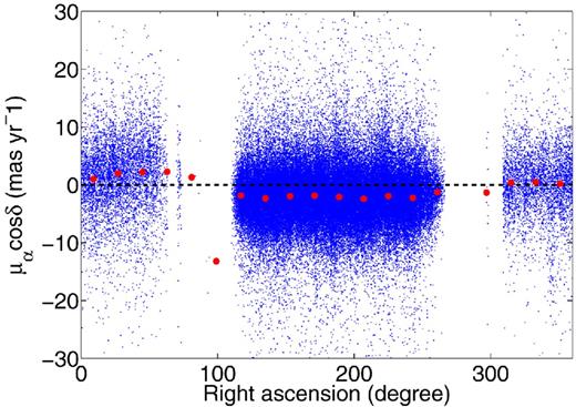
The proper motions of QSOs in the PPMXL catalogue. The black dashed line indicates zero systematics. The red points show the median values in each bin of right ascension.
Since the systematic errors are correlated with position, we need to correct the proper motions of stars. For each star, first, we find the quasars within a circle of diameter 2°. Then, as a subsample, we calculate their median value and dispersion. The median value is used to correct the proper motion, and the dispersion is used as the error of the proper motion. The errors are typically around 4 mas yr− 1.
APPENDIX B: THE CHOICE OF THE NUMBER OF GAUSSIANS IN THE RECONSTRUCTED U–V DISTRIBUTION
Two parameters determine the reconstructed U–V distribution assembled by multiple Gaussians, namely the regularization parameter, w, and the number of Gaussians, K. The former has been discussed in Section 2, in this section we discuss how to determine the latter, K. In principle, the larger K used in the model, the better it can fit the data. In practice, too many Gaussians increase the complexity and some may follow the statistical fluctuations, leading to overfitting. Therefore, we need to determine how many Gaussians are suitable for our mixed model.
There are multiple means to provide statistically optimized choice of K according to Bovy et al. (2009). These are split out into internal and external means. The internal means provide certain criteria that can be applied to determine the number of K, e.g. Akaike's information criterion (Akaike 1974), minimum description length (Rissanen 1978; Schwarz 1978), minimum message length (Wallace & Freeman 1987; Oliver & Baxter 1994; Oliver, Baxter & Wallace 1996), and Bayesian evidence (Roberts et al. 1998), etc. However, these criteria usually do not agree with each other. Moreover, Bovy et al. discussed that the unknown covariance in the data may also affect the determination of K. Another kind of means are the external validation. Since the Hipparcos data used by Bovy et al. generally do not have radial velocities, they used the radial velocities provided by GCS catalogue as the external source to validate the velocity distribution model and find the most appropriate K. Because it is one of the most conservative solutions, it seems that the validation test prefers a smaller number of Gaussians in Bovy et al. (2009) and, consequently, it may miss some substructures because of the lack of Gaussians to model them. Moreover, it also relies on the extra information in a subsample, in the case of the data used by Bovy et al. (2009), it relies on the radial velocity of the GCS data. In general, it is difficult to define such a subsample without systematic bias. For our data, since we use all three-dimensional velocities, there is no such extra information which can be applied to validate the best choice for K.
Thus, we turn to another experimental means to determine the value of K for our case. We reconstruct the U–V distribution based on the average distances with K = 5, 10, and 15 Gaussians (see the left-hand column of Fig. B1) and check if the most prominent substructures shown in Fig. 8 also appear when the model contains fewer Gaussians. The left-hand column of Fig. B1 shows that the most interesting features, e.g. right-hand part of 1, 2, and 8, indeed show up even with K = 5. This implies that these prominent features cannot be spurious results due to the use of too many Gaussians.
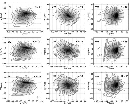
In the left-hand column, the top, middle, and bottom panel shows the U–V distribution with K = 5, 10, and 15 Gaussians respectively. In the middle column, the top, middle, and bottom panel shows the U–W distribution with K = 10, 15, and 18 Gaussians. In the right-hand column, the top, middle, and bottom panel shows the V–W distribution with K = 10, 15, and 18 Gaussians. The contour levels are the same as in Fig. 7. All the results are fitted using the mean distances.
Alternatively, testing the smoothness of U–W and V–W distribution can also qualitatively investigate whether the choice of K is suitable, given the prior knowledge that the velocity U–W and V–W distributions should be smoother than that in the U–V plane. In the middle and right-hand columns of Fig. B1, we show the U–W and V–W distributions with K = 10, 15, and 18 Gaussians, respectively. They show that spurious structures increase with K but do not diffuse to the central region of the U–W and V–W distributions, i.e. 50 km s−1 around the centre, but only contribute to the outskirts, which is mostly due to relatively sparse data there. It is notable that two structures located at (U, W) = (30, −40) and (U, W) = (27, 28) do exist in the U–W distribution when K = 15 and 18, which may indicate two real structures. Because most of the data concentrate in the central region (a 10 km s−1 × 10 km s−1 bin), the signal-to-noise ratio (S/N) of the stellar density in the centre is about 20 according to the Poisson distribution. Hence, statistical fluctuations in the region with such high S/N should be weak and the Gaussians assigned in the central region are unlikely to be affected by the noise. Although W distribution is smoother, the U–W and V–W distributions may still have few structures, such features have also been seen in figs 3 and 4 of Bovy et al. (2009). In the outskirts, on the contrary, since the density is low, the S/N of the stellar density is also low and the fluctuation in this region is mainly arbitrary. When we add more Gaussians in the U–W and V–W distributions, since the central parts are quite smooth and do not need many Gaussians to be fit, the additional Gaussians are assigned to the outskirts to fit the statistical fluctuations and create possible, spurious structures. That is, spurious structures may first occur in the region with lowest S/N of the stellar density; only when the low S/N region has been well covered and if there are still a few Gaussians left, they will tend to overfit the weak arbitrary fluctuations in the high S/N region.
For the case of the U–V distribution, since the central region (with high S/N of the stellar density) does have some substructures, it needs more Gaussians to fit these features and thus not many Gaussians are left to overfit the outskirts. Therefore, we do not see strong spurious structures in the top panel of Fig. 8, implying that the choice of K is suitable for our data. However, when we look at the middle and bottom panels of Fig. 8, because these are the U–V distributions for two subsamples located within and outside the solar circle, respectively, some Gaussians are assigned to their outskirts with lower S/N. Subsequently, these two panels show more spurious structures than the top panel.
Combining these two independent means, we can infer that K = 20 will not produce artificial spurious structures in the central region of the U–V distribution. Given that the prominent substructures shown in the top panel of Fig. 8 have already shown their significance when K is smaller, we believe they are real features.
