Study of morphology and stellar content of the Galactic H ii region IRAS 16148−5011

Mallick, K. K.; Ojha, D. K.; Tamura, M.; Linz, H.; Samal, M. R.; Ghosh, S. K.

doi:10.1093/mnras/stu2584

Abstract

An investigation of the IRAS 16148−5011 region – a cluster at a distance of 3.6 kpc – is presented here, carried out using multiwavelength data in near-infrared (NIR) from the 1.4 m Infrared Survey Facility telescope, mid-infrared (MIR) from the archival Spitzer GLIMPSE (Galactic Legacy Infrared Midplane Survey Extraordinaire) survey, far-infrared (FIR) from the Herschel archive, and low-frequency radio continuum observations at 1280 and 843 MHz from the Giant Metrewave Radio Telescope and Molonglo Survey archive, respectively. A combination of NIR and MIR data is used to identify 7 Class I and 133 Class II sources in the region. Spectral energy distribution (SED) analysis of selected sources reveals a 9.6 M_⊙ high-mass source embedded in nebulosity. However, Lyman continuum luminosity calculation using radio emission – which shows a compact H ii region – indicates the spectral type of the ionizing source to be earlier than B0-O9.5. Free–free emission SED modelling yields the electron density as 138 cm⁻³, and thus the mass of the ionized hydrogen as ∼16.4 M_⊙. Thermal dust emission modelling, using the FIR data from Herschel and performing modified blackbody fits, helped us construct the temperature and column density maps of the region, which show peak values of 30 K and 3.3 × 10²² cm⁻², respectively. The column density maps reveal an A_V > 20 mag extinction associated with the nebular emission, and weak filamentary structures connecting dense clumps. The clump associated with this IRAS object is found to have dimensions of ∼ 1.1 pc × 0.8 pc, and a mass of 1023 M_⊙.

stars: formation, dust, extinction, H ii regions, ISM: individual objects: IRAS 16148−5011, infrared: ISM, radio continuum: ISM

1 INTRODUCTION

Most star formation activity is known to take place in clusters (Lada & Lada 2003), and as such, observational studies of young embedded stellar cluster regions are imperative, because they serve as a template to further investigate various associated processes and their signatures. Due to the youth of such regions and the fact that their natal medium has still not been dispersed, these clusters can be used to scrutinize various theories related to star formation, stellar cluster dynamics, as well as stellar and cloud evolution. Of even more importance are the cluster regions which harbour high-mass stars, partly because such regions are few and far between, and more so as high-mass star formation is not very well understood (Zinnecker & Yorke 2007).

IRAS 16148−5011 is an infrared nebula (Fig. 1) in the southern sky (α₂₀₀₀ = 16^h18^m35|${^{\rm s}_{.}}$|2, δ₂₀₀₀ = −50°18^′53^′^′) associated with which is an IR cluster found using the Two Micron All-Sky Survey (2MASS) data by Dutra et al. (2003). It is located at the Galactic plane (l ∼ 333| $_{.}^{\circ}$|047, b ∼ +0| $_{.}^{\circ}$|037) and is in the vicinity of the well-known star-forming region RCW 106. Though other star-forming regions are present nearby, IRAS 16148−5011 appeared to be a relatively isolated region in past mappings (Karnik et al. 2001; Mookerjea et al. 2004). Kinematic distance estimates to this region vary from ∼3.3 to 11.9 kpc (near- and far-distance estimates; Molinari et al. 2008), and we adopt the distance of 3.6 kpc from Lumsden et al. (2013, based on the spectrophotometric distance of a prominent source – ‘G333.0494+00.0324B’ in their nomenclature – associated with the central nebula¹) for our work. The compilation of Lumsden et al. (2013) also reveals other nearby regions at this distance, providing preliminary indications that this could be a part of larger complex. In the early analyses of Haynes, Caswell & Simons (1979, also see Chan, Henning & Schreyer 1996), radio continuum emission at 6 cm was detected, with peak in the neighbourhood (≳1 arcmin, positional accuracy ∼30 arcsec) of this region, and it was predicted to be harbouring massive young stellar objects (YSOs). The IRAS colour analysis by MacLeod et al. (1998) was also found to be consistent with that for an H ii region, and Molinari et al. (2008) – using the IRAS ‘[25−12]’ colour value – have suggested that this region is among the younger IRAS-detected regions. A high-mass stellar source was detected by Grave & Kumar (2009) with the help of spectral energy distribution (SED) fitting using near-infrared (NIR) to millimetre (mm) data. Analyses of this region at 1.2-mm dust continuum emission and at molecular lines have revealed the presence of dense gas, with a large column density, as well as massive clumps. The total luminosity estimate (∼4.4 × 10⁴ L_⊙, by integrating IRAS flux densities) has also been found to be well in the regime of high-mass stellar objects (Fontani et al. 2005; Beltrán et al. 2006). Therefore, taking into account these characteristics, this region makes a good candidate to carry out an investigation for understanding the morphology and stellar population. However, since this is a possible H ii region with an embedded cluster, multiwavelength observations are required to fully discern this region's various constituents and how they relate to each other. In this paper, we have tried to accomplish this using deep NIR observations, archival mid-infrared (MIR) Spitzer data, archival far-infrared (FIR) Herschel data, and low-frequency radio continuum observations.

Figure 1.

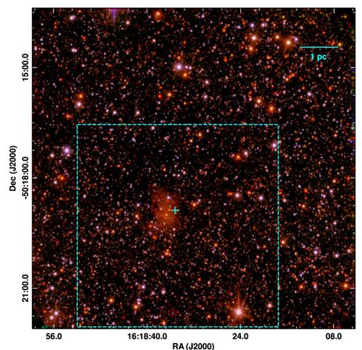
Colour composite image of the IRAS 16148−5011 region, made using the K_s (red), H (green), and J (blue) band images. The area of analysis in this paper has been marked by the dashed rectangle. Plus symbol marks the IRAS catalogue position of IRAS 16148−5011. The scale bar shows 1 pc extent at a distance of 3.6 kpc.

Open in new tab Download slide

In Section 2, we detail the various observations and the corresponding data analysis procedures, followed by an examination of the stellar population in the region in Section 3. The morphology of the region is discussed in Section 4. Discussion and conclusions are presented in Sections 5 and 6, respectively.

2 OBSERVATIONS AND DATA REDUCTION

2.1 NIR observations

NIR photometric observations in J (1.25 μm), H (1.63 μm), and K_s (2.14 μm) bands (centred on α₂₀₀₀ ∼ 16^h18^m31^s, δ₂₀₀₀ ∼ −50°17^′32^′^′) were carried out on 2004 July 29 using the 1.4 m Infrared Survey Facility (IRSF) telescope, South Africa. The observations were taken with the help of the Simultaneous InfraRed Imager for Unbiased Survey (SIRIUS) instrument, a three colour simultaneous camera mounted at the f/10 Cassegrain focus of the telescope. SIRIUS is equipped with three 1k × 1k HgCdTe arrays, each of which, with a pixel scale of 0.45 arcsec, provide a field of view (FoV) of 7.8 arcmin × 7.8 arcmin. Further details can be obtained from Nagashima et al. (1999) and Nagayama et al. (2003). Five sets of frames, with each set containing observations at ten dithered positions (exposure time of 5 s at each dither position), were obtained (i.e. total exposure time = 5 × 10 × 5 s = 250 s, in each band). The sky conditions were photometric, with a seeing size of ∼1.35 arcsec. In addition to the target field, a sky region (∼10 arcmin to the north of target region) and the standard star P9172 (Persson et al. 1998) were also observed.

Following a standard data reduction procedure, which involved bad pixel masking, dark subtraction, flat-field correction, sky subtraction, combining dithered frames, and astrometric calibration, point spread function (psf) photometry was carried out using the ALLSTAR algorithm of the daophot package in iraf. About 11–13 sources were used to construct the psf for each band. Finally, the instrumental magnitudes were calibrated using the standard star P9172. The astrometric calibration rms obtained was <0.05 arcsec, and the median photometric error <0.05 mag. On comparing our catalogues with the 2MASS catalogues, sources with K_s magnitude ≤ 9.5 were found to be saturated, and hence had their J, H, and K_s magnitudes replaced by the corresponding 2MASS magnitudes. The final NIR catalogue is used to identify the YSOs in the region. The area of study in this paper is about 5.5 arcmin × 5.5 arcmin encompassing the nebular cloud region, centred on α₂₀₀₀ ∼ 16^h18^m35^s, δ₂₀₀₀ ∼ −50°19′18′′.

Completeness limits were calculated for all three bands by carrying out artificial star experiments using the addstar package in iraf. A fixed number of stars were added in each 0.5 mag bin and analysis carried out to see how many stars are detected. The ratio of the number of detected stars to the number of added stars gives us the completeness fraction as a function of magnitude. The 90 per cent completeness limit was thus calculated as 16.6, 15.8, and 15.5 for the J, H, and K_s bands, respectively.

2.2 Radio continuum observations

Radio continuum observations at 1280 MHz were obtained on 2012 November 09 using the Giant Metrewave Radio Telescope (GMRT) array. The GMRT array consists of 30 antennas arranged in an approximate Y-shaped configuration, with each antenna having a diameter of 45 m. This translates to a primary beam-size of 26.2 arcmin at 1280 MHz. A central region of ∼1 km × 1 km contains 12 randomly distributed antennas, while the remaining 18 are along the three radial arms (six along each arm) which extend up to ∼14 km. Details about the GMRT can be found in Swarup et al. (1991).

For our observations, the Very Large Array phase and flux calibrators ‘1626-298’ and ‘3C286’, respectively, were used. The total observation time (including the calibrators) was about 3.5 h, limited by the low declination of the source. Data reduction was carried out using the aips software. Initial steps involved flagging the bad data (carried out using a combination of ‘vplot-uvflg’ and ‘tvflg’ tasks) and calibration (carried out using ‘calib-getjy-clcal’). After a few iterations of flagging and calibration, the source data were ‘split’ from the whole, and were used for imaging using the task ‘imagr’. A few rounds of (phase) self-calibration were also carried out using the task ‘calib’ to remove any ionospheric phase distortion effects. To check that the flux calibration was done correctly, the image of the flux calibrator was constructed, and its flux determined and checked against literature values. The final (target) source images were rescaled to take into account the system temperature corrections for the GMRT. These corrections are required as, at the Galactic plane, the large amount of radiation at metre wavelengths increases the effective temperature of the antennas. This was done as follows. Using the sky temperature map of Haslam et al. (1982) at 408 MHz, and the spectral index of −2.6 given therein, the temperature towards this region was obtained, i.e. T_frequency = T₄₀₈ × (frequency/408 MHz)^−2.6, where T₄₀₈ is the temperature at 408 MHz and T_frequency is the temperature at required frequency (1280 MHz here). The images were subsequently rescaled by a factor given by (T_frequency + T_sys)/T_sys, i.e. the ratio of temperature towards the target to that towards the flux calibrator. T_sys, the system temperature, was obtained from the GMRT manual.²

In addition to the GMRT observations, we also obtained the archival first epoch Molongolo Galactic Plane Survey (MGPS) data at 843 MHz³ (Green et al. 1999). The MGPS observations were carried out using the Molonglo Observatory Synthesis Telescope (MOST)⁴ with a resolution of 43 arcsec × 43 arcsec cosec |Declination|. For our analysis purpose, we retrieved the original processed image for this region's Galactic coordinates (resolution ∼ 55.84 arcsec× 43 arcsec) from the website. The radio images are used to obtain the physical parameters and examine the morphology of the ionized gas in the region (see Section 4.2).

2.3 Other archival data sets

2.3.1 Spitzer MIR observations

Archival MIR observations of this region, obtained using the Spitzer Space Telescope under the Galactic Legacy Infrared Midplane Survey Extraordinaire (GLIMPSE) programme (Benjamin et al. 2003; Churchwell et al. 2009), were retrieved with the help of the InfraRed Science Archive⁵ (the Spring’07 Archive more complete catalogue). GLIMPSE observations were taken using the InfraRed Array Camera (IRAC) in 3.6, 4.5, 5.8, and 8.0 μm bands. The final image cutouts (pixel scale of 0.6 arcsec) as well as the final catalogues were downloaded. While the images are further used to analyse features in the region, the photometric catalogue, in conjunction with the NIR catalogue (Section 2.1) was used to identify the YSOs in the region.

2.3.2 Herschel FIR observations

This region has been observed at FIR wavelengths, in the range 70–500 μm, using the instruments Photodetector Array Camera and Spectrometer (PACS; Poglitsch et al. 2010) and Spectral and Photometric Imaging Receiver (SPIRE; Griffin et al. 2010) on the 3.5-m Herschel Space Observatory (Pilbratt et al. 2010), as a part of the Proposal ID ‘KPOT_smolinar_1’ (Molinari et al. 2010). For our analyses, we obtained the PACS 70- and 160-μm level2_5 MADmap images (Cantalupo et al. 2010); and the SPIRE 250-, 350-, and 500-μm level2_5 extended source (‘extdPxW’) map products using the Herschel Science Archive.⁶ The 70, 160, 250, 350, and 500 μm images have pixel scales of 3.2, 6.4, 6, 10, and 14 arcsec, respectively, with resolutions varying from ∼5.5–36 arcsec. While the PACS image obtained had the surface brightness unit of Jy pixel⁻¹, the SPIRE images were in the units of MJy sr⁻¹. Detailed information about the data products is provided on the Herschel site.⁷ We use the FIR data to examine the physical conditions of the region.

3 STELLAR POPULATION IN THE REGION

3.1 Identification of YSOs

The NIR and MIR photometric catalogues from IRSF (Section 2.1) and GLIMPSE (Section 2.3.1), respectively, were cross-matched within 0.6 arcsec matching radius and collated to obtain a combined photometric catalogue. Thereafter, the following set of steps were followed for the identification of the YSOs (similar to Mallick et al. 2013).

First, the YSOs were identified using their MIR magnitudes. The sources with detections in all four IRAC bands with errors ≤ 0.15 mag were used here. Using simple linear regression, the IRAC spectral index (α_IRAC = dlog (λF_λ)/dlog (λ); Lada 1987) was calculated for each source (in the wavelength range 3.6–8.0 μm), followed by their classification into Class I and Class II categories using the limits from Chavarría et al. (2008, α_IRAC > 0 for Class I, and −2 ≤ α_IRAC ≤ 0 for Class II; see Fig. 2a).
All sources need not have detections at 5.8 and 8.0 μm, but might have good quality detections in NIR bands. To identify the YSOs from amongst such sources, we use a combination of H, K_s, 3.6 μm, and 4.5 μm bands following the procedure of Gutermuth et al. (2009). Again, only those sources whose 3.6- and 4.5-μm magnitude errors are ≤0.15 are used here. The YSOs were identified from their location in the dereddened – using the colour excess ratios from Flaherty et al. (2007) – ‘K_s–[3.6]’ versus ‘[3.6]–[4.5]’ colour–colour diagram (CCD), as is shown in Fig. 2(b).
Additional YSOs were identified using the J − H/H − K CCD (Fig. 2c) according to the following procedure. In Fig. 2(c), the red solid curve marks the dwarf locus from Bessell & Brett (1988) and the blue solid line marks the Classical T Tauri Stars (CTTS) locus from Meyer, Calvet & Hillenbrand (1997). All the loci curves as well as sources’ colours were converted to CIT (California Institute of Technology) photometric system (using Carpenter 2001) for this analysis. The slanted dashed lines are the reddening vectors, drawn using the reddening laws of Cohen et al. (1981) for the CIT photometric system. In this CCD, three separate regions have been marked, similar to Ojha et al. (2004a,b). The sources in ‘T’ and ‘P’ regions are taken to be Class II sources (Lada & Adams 1992), as they exhibit IR-excess emission. In the ‘P’ region, since there could be a slight overlap between Herbig Ae/Be stars and Class II sources (Hillenbrand et al. 1992), we conservatively took only those sources which were above the CTTS locus extended into this region (similar to Mallick et al. 2014). It should be noted that sources in the ‘T’ region could also contain a few Class III sources with small IR-excess.

Figure 2.

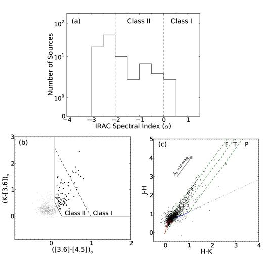
(a) Histogram of the IRAC spectral indices. The limits for Class I and Class II sources have been marked by dashed grey vertical lines. (b) NIR–MIR CCD using the procedure of Gutermuth et al. (2009). The regions of Class I and Class II sources have been labelled. The identified YSOs have been shown with black solid circles. (c) NIR CCD in CIT system. The red curve and the blue line show the dwarf locus (Bessell & Brett 1988) and the CTTS locus (Meyer et al. 1997), respectively. The grey dot–dashed line is the extension of CTTS locus. Three parallel slanted dashed lines mark the reddening vectors, drawn using extinction laws from Cohen et al. (1981). Three separate regions, ‘F’, ‘T’, ‘P’ have been labelled on the plot. The source marked with a cross in ‘P’ region is a high-mass YSO (see text).

Open in new tab Download slide

Finally, we merged the sources identified in each step. An overlapping source might have different identifications in different steps. Thus, in the final list, the class of a YSO was taken as that in which it was identified as first in the above order of steps. A total of 7 Class I and 133 Class II sources were obtained (for a FoV of ∼5.5 arcmin × 5.5 arcmin encompassing the molecular cloud, as marked in Fig. 1) in the final YSO catalogue, which is given in Table 1.

Table 1.

Open in new tab

YSOs identified using NIR and MIR data.

RA	Dec.	J	H	K_s	[3.6]	[4.5]	[5.8]	[8.0]	YSO
(J2000)	(J2000)	(mag)	(mag)	(mag)	(mag)	(mag)	(mag)	(mag)	classification
244.575 165	−50.365 025	17.861 ± 0.130	16.631 ± 0.001	15.509 ± 0.047	14.311 ± 0.145	14.132 ± 0.203	–	–	Class2
244.575 241	−50.367 393	14.580 ± 0.021	13.876 ± 0.010	13.643 ± 0.032	12.983 ± 0.099	12.872 ± 0.122	–	–	Class2
244.576 645	−50.293 938	16.137 ± 0.016	14.443 ± 0.010	13.570 ± 0.020	12.780 ± 0.102	12.372 ± 0.132	–	–	Class2
244.577 545	−50.314 171	15.557 ± 0.010	14.358 ± 0.010	13.818 ± 0.028	13.001 ± 0.108	12.820 ± 0.143	–	–	Class2
244.579 193	−50.321 396	17.491 ± 0.045	15.921 ± 0.020	14.881 ± 0.038	13.412 ± 0.161	13.265 ± 0.132	–	–	Class2

RA	Dec.	J	H	K_s	[3.6]	[4.5]	[5.8]	[8.0]	YSO
(J2000)	(J2000)	(mag)	(mag)	(mag)	(mag)	(mag)	(mag)	(mag)	classification
244.575 165	−50.365 025	17.861 ± 0.130	16.631 ± 0.001	15.509 ± 0.047	14.311 ± 0.145	14.132 ± 0.203	–	–	Class2
244.575 241	−50.367 393	14.580 ± 0.021	13.876 ± 0.010	13.643 ± 0.032	12.983 ± 0.099	12.872 ± 0.122	–	–	Class2
244.576 645	−50.293 938	16.137 ± 0.016	14.443 ± 0.010	13.570 ± 0.020	12.780 ± 0.102	12.372 ± 0.132	–	–	Class2
244.577 545	−50.314 171	15.557 ± 0.010	14.358 ± 0.010	13.818 ± 0.028	13.001 ± 0.108	12.820 ± 0.143	–	–	Class2
244.579 193	−50.321 396	17.491 ± 0.045	15.921 ± 0.020	14.881 ± 0.038	13.412 ± 0.161	13.265 ± 0.132	–	–	Class2

Note. Table 1 is available in its entirety in a machine-readable form in the online journal. A portion is shown here for guidance regarding its form and content.

Table 1.

Open in new tab

YSOs identified using NIR and MIR data.

RA	Dec.	J	H	K_s	[3.6]	[4.5]	[5.8]	[8.0]	YSO
(J2000)	(J2000)	(mag)	(mag)	(mag)	(mag)	(mag)	(mag)	(mag)	classification
244.575 165	−50.365 025	17.861 ± 0.130	16.631 ± 0.001	15.509 ± 0.047	14.311 ± 0.145	14.132 ± 0.203	–	–	Class2
244.575 241	−50.367 393	14.580 ± 0.021	13.876 ± 0.010	13.643 ± 0.032	12.983 ± 0.099	12.872 ± 0.122	–	–	Class2
244.576 645	−50.293 938	16.137 ± 0.016	14.443 ± 0.010	13.570 ± 0.020	12.780 ± 0.102	12.372 ± 0.132	–	–	Class2
244.577 545	−50.314 171	15.557 ± 0.010	14.358 ± 0.010	13.818 ± 0.028	13.001 ± 0.108	12.820 ± 0.143	–	–	Class2
244.579 193	−50.321 396	17.491 ± 0.045	15.921 ± 0.020	14.881 ± 0.038	13.412 ± 0.161	13.265 ± 0.132	–	–	Class2

RA	Dec.	J	H	K_s	[3.6]	[4.5]	[5.8]	[8.0]	YSO
(J2000)	(J2000)	(mag)	(mag)	(mag)	(mag)	(mag)	(mag)	(mag)	classification
244.575 165	−50.365 025	17.861 ± 0.130	16.631 ± 0.001	15.509 ± 0.047	14.311 ± 0.145	14.132 ± 0.203	–	–	Class2
244.575 241	−50.367 393	14.580 ± 0.021	13.876 ± 0.010	13.643 ± 0.032	12.983 ± 0.099	12.872 ± 0.122	–	–	Class2
244.576 645	−50.293 938	16.137 ± 0.016	14.443 ± 0.010	13.570 ± 0.020	12.780 ± 0.102	12.372 ± 0.132	–	–	Class2
244.577 545	−50.314 171	15.557 ± 0.010	14.358 ± 0.010	13.818 ± 0.028	13.001 ± 0.108	12.820 ± 0.143	–	–	Class2
244.579 193	−50.321 396	17.491 ± 0.045	15.921 ± 0.020	14.881 ± 0.038	13.412 ± 0.161	13.265 ± 0.132	–	–	Class2

Note. Table 1 is available in its entirety in a machine-readable form in the online journal. A portion is shown here for guidance regarding its form and content.

3.2 SED of YSOs

SED modelling was carried out for (a subset of) YSOs to get estimates of their physical parameters. The grid of YSO models from Robitaille et al. (2006) – implemented in the online SED fitting tool of Robitaille et al. (2007) – was used for this purpose. The basic model consists of a pre-main sequence (PMS) star surrounded by a flared accretion disc having a rotationally flattened envelope with cavities carved out by a bipolar outflow. A total of 200 000 SED models are computed in a 14D parameter space (covering properties of the central source, the infalling envelope, and the disc), using the radiation transfer code of Whitney et al. (2003a,b). The online fitting tool attempts to fit the available SED models to the data, characterizing each fitting by a χ² parameter. The distance range and the interstellar visual extinction (A_V) are free parameters whose range has to be specified by the user. Accounting for the uncertainties, we adopted a large distance range of 3.4 to 3.8 kpc for our sources. From extinction calculations (see Section 4.1), we find that almost all non-YSO sources had A_V ≤ 20 mag, and thus we specified the range of interstellar visual extinction A_V as 1–20 mag.

Since the number of SED models is very large, spanning a wide range of parameter space, the models fitting each source can only be constrained by increasing the number of data points used, and having data points to sufficiently cover the entire wavelength range of fitting. For this reason, we choose the sources with photometry in at least all four IRAC bands for SED modelling. However, in addition to those selected using this criterion, we also carried out SED analysis for the prominent sources associated with the central nebula (even though two of them lacked 8.0 μm photometry). We note that photometry from Herschel images is not useful here as none of the YSOs have counterparts at those wavelengths, which in part is due to poor resolution.

For each source, the SED fitting tool – besides giving the best-fitting model – also gives a set of well-fitted models ranked by their χ² values as a measure of their relative ‘goodness-of-fit’. Following a method similar to Robitaille et al. (2007), we consider only those models for further calculation which satisfied the following criterion:

\begin{equation} \chi ^{2} - \chi ^{2}_{{\rm min}} < 3 \ \rm {(per\ data\ point)}. \end{equation}

(1)

As elucidated in Robitaille et al. (2007), though this criterion is based on visual examination of SED plots and has no rigid mathematical backing, a stricter criterion might lead to overinterpretation. For each parameter, the weighted mean value and standard deviation were calculated using the models which satisfied equation (1). The inverse of the respective χ² was taken as the weight for each model (similar to Grave & Kumar 2009). Table 2 gives our SED modelling results, listing the physical parameters: age of the central source (T_⋆), mass of the central source, disc mass (M_disc), disc accretion rate (⁠|$\dot{M}_{{\rm disc}}$|⁠), envelope mass (M_env), temperature of the central source (T_⋆), total system luminosity (L_total), interstellar visual extinction (A_V), and the |$\chi ^{2}_{{\rm min}}$| per data point. Errors for some parameters tend to be large as we are dealing with a large parameter space while we have very few data points to constrain the number of models. If a source was simply fit better as a star with high interstellar extinction, it has not been included in the table. Thus finally, SED results are given for a total of three Class I sources, 24 Class II sources (including two central sources), and one extra central source.

Table 2.

Open in new tab

Main parameters from SED analysis.

S.No.	RA	Dec.	log T_⋆	Mass	log M_disc	\|$\log \,\dot{M}_{{\rm disc}}$\|	log M_env	log T_⋆	log L_total	A_V	\|$\chi _{min}^2$\|
	(J2000)	(J2000)	(yr)	(M_⊙)	(M_⊙)	(M_⊙ yr⁻¹)	(M_⊙)	(K)	(L_⊙)	(mag)	(per data point)
Class I sources
1	244.591 080	−50.285 355	6.33 ± 0.74	2.42 ± 0.79	−3.38 ± 1.64	−9.29 ± 1.73	−4.43 ± 2.73	3.85 ± 0.15	1.41 ± 0.30	4.81 ± 2.35	0.29
2	244.603 455	−50.292 828	4.71 ± 0.40	4.20 ± 1.42	−1.39 ± 0.70	−6.70 ± 0.99	0.68 ± 1.06	3.66 ± 0.07	2.11 ± 0.28	15.95 ± 4.98	0.01
3	244.671 539	−50.338 348	5.30 ± 1.02	2.58 ± 1.61	−2.90 ± 1.82	−8.08 ± 2.02	−2.70 ± 2.90	3.73 ± 0.20	1.56 ± 0.56	7.45 ± 4.16	0.10
Class II sources
4	244.584 152	−50.353 664	4.65 ± 0.37	6.41 ± 0.54	−2.12 ± 0.75	−6.94 ± 0.80	1.65 ± 0.40	3.66 ± 0.01	2.49 ± 0.06	12.17 ± 5.81	9.90
5	244.599 808	−50.286 560	4.94 ± 0.37	3.80 ± 1.81	−1.99 ± 0.84	−7.55 ± 1.30	0.54 ± 0.66	3.66 ± 0.05	1.93 ± 0.41	11.51 ± 5.27	1.93
6	244.606 796	−50.307 327	5.57 ± 0.87	7.50 ± 3.12	−4.67 ± 2.72	−9.18 ± 2.08	−3.10 ± 4.21	4.02 ± 0.35	2.95 ± 0.68	13.72 ± 5.07	5.34
7	244.609 207	−50.351 631	4.97 ± 0.27	4.68 ± 1.40	−2.11 ± 0.93	−7.66 ± 1.31	1.24 ± 0.53	3.67 ± 0.05	2.12 ± 0.32	17.37 ± 3.72	10.85
8	244.610 397	−50.279 411	5.14 ± 0.76	2.99 ± 1.59	−2.25 ± 0.95	−7.76 ± 1.28	−0.70 ± 2.22	3.70 ± 0.15	1.73 ± 0.36	13.43 ± 5.74	0.29
9	244.612 305	−50.365 067	4.84 ± 0.45	5.60 ± 2.59	−2.04 ± 1.05	−7.61 ± 1.55	1.09 ± 0.87	3.70 ± 0.07	2.31 ± 0.66	4.51 ± 2.81	0.34
10	244.614 349	−50.327 496	6.28 ± 0.66	2.50 ± 0.83	−3.40 ± 1.71	−9.21 ± 1.89	−4.37 ± 2.56	3.85 ± 0.17	1.44 ± 0.35	6.20 ± 2.30	0.13
11	244.633 514	−50.326 122	5.73 ± 0.70	2.58 ± 0.99	−3.20 ± 1.77	−8.84 ± 1.80	−2.83 ± 2.80	3.77 ± 0.19	1.54 ± 0.35	8.83 ± 4.50	0.28
12	244.639 954	−50.283 981	5.10 ± 0.07	4.80 ± 0.22	−2.36 ± 0.66	−7.50 ± 0.20	1.14 ± 0.56	3.66 ± 0.01	2.02 ± 0.07	9.75 ± 5.38	2.16
13^{a, b}	244.644 714	−50.314 804	4.18 ± 1.01	6.17 ± 1.74	–	–	−0.18 ± 1.92	3.76 ± 0.26	2.82 ± 0.31	6.18 ± 3.86	0.03
14	244.649 155	−50.346 909	5.65 ± 0.90	2.44 ± 1.12	−2.92 ± 1.44	−8.40 ± 1.68	−2.87 ± 3.05	3.79 ± 0.20	1.58 ± 0.35	7.63 ± 4.29	0.03
15	244.651 047	−50.328 751	6.29 ± 0.68	3.46 ± 0.86	−3.43 ± 1.48	−8.96 ± 1.60	−4.83 ± 2.75	3.99 ± 0.18	2.01 ± 0.27	6.70 ± 2.41	0.13
16^{a, c}	244.652 878	−50.316 849	5.44 ± 0.61	9.60 ± 1.44	−2.15 ± 1.24	−7.00 ± 1.35	0.00 ± 3.42	4.29 ± 0.20	3.69 ± 0.16	15.97 ± 4.36	0.89
17	244.663 803	−50.352 959	6.02 ± 0.78	2.93 ± 0.82	−3.23 ± 1.35	−8.92 ± 1.53	−3.75 ± 3.08	3.86 ± 0.19	1.74 ± 0.24	4.75 ± 2.79	0.07
18	244.671 738	−50.278 400	5.30 ± 0.28	3.02 ± 1.19	−2.97 ± 1.18	−8.96 ± 1.72	−0.74 ± 0.91	3.67 ± 0.05	1.62 ± 0.27	10.13 ± 3.37	3.23
19	244.679 535	−50.293 499	4.97 ± 0.36	4.10 ± 1.47	−2.07 ± 0.86	−7.70 ± 1.19	0.45 ± 0.86	3.67 ± 0.06	2.01 ± 0.30	9.06 ± 5.71	2.25
20	244.685 440	−50.357 010	6.29 ± 0.72	3.69 ± 0.99	−3.83 ± 1.67	−9.31 ± 1.77	−5.06 ± 2.77	4.03 ± 0.19	2.14 ± 0.32	9.15 ± 3.12	0.17
21	244.689 316	−50.343 143	4.99 ± 0.39	3.85 ± 1.38	−2.13 ± 0.83	−7.74 ± 1.20	0.28 ± 1.05	3.67 ± 0.06	1.94 ± 0.26	7.45 ± 5.58	2.23
22	244.689 453	−50.366 440	4.90 ± 0.48	4.06 ± 1.33	−1.97 ± 0.87	−7.40 ± 1.17	0.37 ± 1.39	3.67 ± 0.09	2.04 ± 0.26	13.02 ± 5.40	0.17
23	244.693 146	−50.279 778	5.50 ± 0.67	2.95 ± 0.96	−2.39 ± 0.94	−8.01 ± 1.08	−1.47 ± 2.53	3.73 ± 0.16	1.68 ± 0.19	7.19 ± 3.64	4.84
24	244.704 742	−50.351 349	4.78 ± 0.39	5.70 ± 0.86	−2.26 ± 0.30	−7.61 ± 0.94	1.65 ± 0.30	3.66 ± 0.02	2.37 ± 0.09	17.61 ± 2.63	14.26
25	244.708 603	−50.286 385	4.89 ± 0.35	4.59 ± 1.48	−1.92 ± 0.84	−7.52 ± 1.14	0.89 ± 0.71	3.67 ± 0.06	2.14 ± 0.34	12.96 ± 5.63	3.55
26	244.683 786	−50.363 702	4.75 ± 0.39	6.24 ± 2.25	−1.56 ± 0.82	−6.91 ± 1.09	1.25 ± 0.72	3.71 ± 0.11	2.52 ± 0.51	6.59 ± 5.53	1.57
27	244.687 016	−50.353 573	5.46 ± 0.73	2.87 ± 1.67	−2.60 ± 1.34	−8.20 ± 1.54	−1.73 ± 2.66	3.74 ± 0.16	1.62 ± 0.50	12.36 ± 6.40	0.01
Extra central source
28^{a, b}	244.650 894	−50.314 579	6.17 ± 0.35	8.48 ± 1.17	−4.25 ± 1.30	−9.31 ± 1.32	−4.20 ± 3.65	4.36 ± 0.06	3.52 ± 0.21	18.38 ± 2.26	3.09

S.No.	RA	Dec.	log T_⋆	Mass	log M_disc	\|$\log \,\dot{M}_{{\rm disc}}$\|	log M_env	log T_⋆	log L_total	A_V	\|$\chi _{min}^2$\|
	(J2000)	(J2000)	(yr)	(M_⊙)	(M_⊙)	(M_⊙ yr⁻¹)	(M_⊙)	(K)	(L_⊙)	(mag)	(per data point)
Class I sources
1	244.591 080	−50.285 355	6.33 ± 0.74	2.42 ± 0.79	−3.38 ± 1.64	−9.29 ± 1.73	−4.43 ± 2.73	3.85 ± 0.15	1.41 ± 0.30	4.81 ± 2.35	0.29
2	244.603 455	−50.292 828	4.71 ± 0.40	4.20 ± 1.42	−1.39 ± 0.70	−6.70 ± 0.99	0.68 ± 1.06	3.66 ± 0.07	2.11 ± 0.28	15.95 ± 4.98	0.01
3	244.671 539	−50.338 348	5.30 ± 1.02	2.58 ± 1.61	−2.90 ± 1.82	−8.08 ± 2.02	−2.70 ± 2.90	3.73 ± 0.20	1.56 ± 0.56	7.45 ± 4.16	0.10
Class II sources
4	244.584 152	−50.353 664	4.65 ± 0.37	6.41 ± 0.54	−2.12 ± 0.75	−6.94 ± 0.80	1.65 ± 0.40	3.66 ± 0.01	2.49 ± 0.06	12.17 ± 5.81	9.90
5	244.599 808	−50.286 560	4.94 ± 0.37	3.80 ± 1.81	−1.99 ± 0.84	−7.55 ± 1.30	0.54 ± 0.66	3.66 ± 0.05	1.93 ± 0.41	11.51 ± 5.27	1.93
6	244.606 796	−50.307 327	5.57 ± 0.87	7.50 ± 3.12	−4.67 ± 2.72	−9.18 ± 2.08	−3.10 ± 4.21	4.02 ± 0.35	2.95 ± 0.68	13.72 ± 5.07	5.34
7	244.609 207	−50.351 631	4.97 ± 0.27	4.68 ± 1.40	−2.11 ± 0.93	−7.66 ± 1.31	1.24 ± 0.53	3.67 ± 0.05	2.12 ± 0.32	17.37 ± 3.72	10.85
8	244.610 397	−50.279 411	5.14 ± 0.76	2.99 ± 1.59	−2.25 ± 0.95	−7.76 ± 1.28	−0.70 ± 2.22	3.70 ± 0.15	1.73 ± 0.36	13.43 ± 5.74	0.29
9	244.612 305	−50.365 067	4.84 ± 0.45	5.60 ± 2.59	−2.04 ± 1.05	−7.61 ± 1.55	1.09 ± 0.87	3.70 ± 0.07	2.31 ± 0.66	4.51 ± 2.81	0.34
10	244.614 349	−50.327 496	6.28 ± 0.66	2.50 ± 0.83	−3.40 ± 1.71	−9.21 ± 1.89	−4.37 ± 2.56	3.85 ± 0.17	1.44 ± 0.35	6.20 ± 2.30	0.13
11	244.633 514	−50.326 122	5.73 ± 0.70	2.58 ± 0.99	−3.20 ± 1.77	−8.84 ± 1.80	−2.83 ± 2.80	3.77 ± 0.19	1.54 ± 0.35	8.83 ± 4.50	0.28
12	244.639 954	−50.283 981	5.10 ± 0.07	4.80 ± 0.22	−2.36 ± 0.66	−7.50 ± 0.20	1.14 ± 0.56	3.66 ± 0.01	2.02 ± 0.07	9.75 ± 5.38	2.16
13^{a, b}	244.644 714	−50.314 804	4.18 ± 1.01	6.17 ± 1.74	–	–	−0.18 ± 1.92	3.76 ± 0.26	2.82 ± 0.31	6.18 ± 3.86	0.03
14	244.649 155	−50.346 909	5.65 ± 0.90	2.44 ± 1.12	−2.92 ± 1.44	−8.40 ± 1.68	−2.87 ± 3.05	3.79 ± 0.20	1.58 ± 0.35	7.63 ± 4.29	0.03
15	244.651 047	−50.328 751	6.29 ± 0.68	3.46 ± 0.86	−3.43 ± 1.48	−8.96 ± 1.60	−4.83 ± 2.75	3.99 ± 0.18	2.01 ± 0.27	6.70 ± 2.41	0.13
16^{a, c}	244.652 878	−50.316 849	5.44 ± 0.61	9.60 ± 1.44	−2.15 ± 1.24	−7.00 ± 1.35	0.00 ± 3.42	4.29 ± 0.20	3.69 ± 0.16	15.97 ± 4.36	0.89
17	244.663 803	−50.352 959	6.02 ± 0.78	2.93 ± 0.82	−3.23 ± 1.35	−8.92 ± 1.53	−3.75 ± 3.08	3.86 ± 0.19	1.74 ± 0.24	4.75 ± 2.79	0.07
18	244.671 738	−50.278 400	5.30 ± 0.28	3.02 ± 1.19	−2.97 ± 1.18	−8.96 ± 1.72	−0.74 ± 0.91	3.67 ± 0.05	1.62 ± 0.27	10.13 ± 3.37	3.23
19	244.679 535	−50.293 499	4.97 ± 0.36	4.10 ± 1.47	−2.07 ± 0.86	−7.70 ± 1.19	0.45 ± 0.86	3.67 ± 0.06	2.01 ± 0.30	9.06 ± 5.71	2.25
20	244.685 440	−50.357 010	6.29 ± 0.72	3.69 ± 0.99	−3.83 ± 1.67	−9.31 ± 1.77	−5.06 ± 2.77	4.03 ± 0.19	2.14 ± 0.32	9.15 ± 3.12	0.17
21	244.689 316	−50.343 143	4.99 ± 0.39	3.85 ± 1.38	−2.13 ± 0.83	−7.74 ± 1.20	0.28 ± 1.05	3.67 ± 0.06	1.94 ± 0.26	7.45 ± 5.58	2.23
22	244.689 453	−50.366 440	4.90 ± 0.48	4.06 ± 1.33	−1.97 ± 0.87	−7.40 ± 1.17	0.37 ± 1.39	3.67 ± 0.09	2.04 ± 0.26	13.02 ± 5.40	0.17
23	244.693 146	−50.279 778	5.50 ± 0.67	2.95 ± 0.96	−2.39 ± 0.94	−8.01 ± 1.08	−1.47 ± 2.53	3.73 ± 0.16	1.68 ± 0.19	7.19 ± 3.64	4.84
24	244.704 742	−50.351 349	4.78 ± 0.39	5.70 ± 0.86	−2.26 ± 0.30	−7.61 ± 0.94	1.65 ± 0.30	3.66 ± 0.02	2.37 ± 0.09	17.61 ± 2.63	14.26
25	244.708 603	−50.286 385	4.89 ± 0.35	4.59 ± 1.48	−1.92 ± 0.84	−7.52 ± 1.14	0.89 ± 0.71	3.67 ± 0.06	2.14 ± 0.34	12.96 ± 5.63	3.55
26	244.683 786	−50.363 702	4.75 ± 0.39	6.24 ± 2.25	−1.56 ± 0.82	−6.91 ± 1.09	1.25 ± 0.72	3.71 ± 0.11	2.52 ± 0.51	6.59 ± 5.53	1.57
27	244.687 016	−50.353 573	5.46 ± 0.73	2.87 ± 1.67	−2.60 ± 1.34	−8.20 ± 1.54	−1.73 ± 2.66	3.74 ± 0.16	1.62 ± 0.50	12.36 ± 6.40	0.01
Extra central source
28^{a, b}	244.650 894	−50.314 579	6.17 ± 0.35	8.48 ± 1.17	−4.25 ± 1.30	−9.31 ± 1.32	−4.20 ± 3.65	4.36 ± 0.06	3.52 ± 0.21	18.38 ± 2.26	3.09

Notes. ^aProminent sources associated with the central nebula; ^bDid not have 8.0-μm photometry; ^cIdentified as ‘G333.0494+00.0324B’ (and also classified as a YSO) in Lumsden et al. (2013).

Table 2.

Open in new tab

Main parameters from SED analysis.

S.No.	RA	Dec.	log T_⋆	Mass	log M_disc	\|$\log \,\dot{M}_{{\rm disc}}$\|	log M_env	log T_⋆	log L_total	A_V	\|$\chi _{min}^2$\|
	(J2000)	(J2000)	(yr)	(M_⊙)	(M_⊙)	(M_⊙ yr⁻¹)	(M_⊙)	(K)	(L_⊙)	(mag)	(per data point)
Class I sources
1	244.591 080	−50.285 355	6.33 ± 0.74	2.42 ± 0.79	−3.38 ± 1.64	−9.29 ± 1.73	−4.43 ± 2.73	3.85 ± 0.15	1.41 ± 0.30	4.81 ± 2.35	0.29
2	244.603 455	−50.292 828	4.71 ± 0.40	4.20 ± 1.42	−1.39 ± 0.70	−6.70 ± 0.99	0.68 ± 1.06	3.66 ± 0.07	2.11 ± 0.28	15.95 ± 4.98	0.01
3	244.671 539	−50.338 348	5.30 ± 1.02	2.58 ± 1.61	−2.90 ± 1.82	−8.08 ± 2.02	−2.70 ± 2.90	3.73 ± 0.20	1.56 ± 0.56	7.45 ± 4.16	0.10
Class II sources
4	244.584 152	−50.353 664	4.65 ± 0.37	6.41 ± 0.54	−2.12 ± 0.75	−6.94 ± 0.80	1.65 ± 0.40	3.66 ± 0.01	2.49 ± 0.06	12.17 ± 5.81	9.90
5	244.599 808	−50.286 560	4.94 ± 0.37	3.80 ± 1.81	−1.99 ± 0.84	−7.55 ± 1.30	0.54 ± 0.66	3.66 ± 0.05	1.93 ± 0.41	11.51 ± 5.27	1.93
6	244.606 796	−50.307 327	5.57 ± 0.87	7.50 ± 3.12	−4.67 ± 2.72	−9.18 ± 2.08	−3.10 ± 4.21	4.02 ± 0.35	2.95 ± 0.68	13.72 ± 5.07	5.34
7	244.609 207	−50.351 631	4.97 ± 0.27	4.68 ± 1.40	−2.11 ± 0.93	−7.66 ± 1.31	1.24 ± 0.53	3.67 ± 0.05	2.12 ± 0.32	17.37 ± 3.72	10.85
8	244.610 397	−50.279 411	5.14 ± 0.76	2.99 ± 1.59	−2.25 ± 0.95	−7.76 ± 1.28	−0.70 ± 2.22	3.70 ± 0.15	1.73 ± 0.36	13.43 ± 5.74	0.29
9	244.612 305	−50.365 067	4.84 ± 0.45	5.60 ± 2.59	−2.04 ± 1.05	−7.61 ± 1.55	1.09 ± 0.87	3.70 ± 0.07	2.31 ± 0.66	4.51 ± 2.81	0.34
10	244.614 349	−50.327 496	6.28 ± 0.66	2.50 ± 0.83	−3.40 ± 1.71	−9.21 ± 1.89	−4.37 ± 2.56	3.85 ± 0.17	1.44 ± 0.35	6.20 ± 2.30	0.13
11	244.633 514	−50.326 122	5.73 ± 0.70	2.58 ± 0.99	−3.20 ± 1.77	−8.84 ± 1.80	−2.83 ± 2.80	3.77 ± 0.19	1.54 ± 0.35	8.83 ± 4.50	0.28
12	244.639 954	−50.283 981	5.10 ± 0.07	4.80 ± 0.22	−2.36 ± 0.66	−7.50 ± 0.20	1.14 ± 0.56	3.66 ± 0.01	2.02 ± 0.07	9.75 ± 5.38	2.16
13^{a, b}	244.644 714	−50.314 804	4.18 ± 1.01	6.17 ± 1.74	–	–	−0.18 ± 1.92	3.76 ± 0.26	2.82 ± 0.31	6.18 ± 3.86	0.03
14	244.649 155	−50.346 909	5.65 ± 0.90	2.44 ± 1.12	−2.92 ± 1.44	−8.40 ± 1.68	−2.87 ± 3.05	3.79 ± 0.20	1.58 ± 0.35	7.63 ± 4.29	0.03
15	244.651 047	−50.328 751	6.29 ± 0.68	3.46 ± 0.86	−3.43 ± 1.48	−8.96 ± 1.60	−4.83 ± 2.75	3.99 ± 0.18	2.01 ± 0.27	6.70 ± 2.41	0.13
16^{a, c}	244.652 878	−50.316 849	5.44 ± 0.61	9.60 ± 1.44	−2.15 ± 1.24	−7.00 ± 1.35	0.00 ± 3.42	4.29 ± 0.20	3.69 ± 0.16	15.97 ± 4.36	0.89
17	244.663 803	−50.352 959	6.02 ± 0.78	2.93 ± 0.82	−3.23 ± 1.35	−8.92 ± 1.53	−3.75 ± 3.08	3.86 ± 0.19	1.74 ± 0.24	4.75 ± 2.79	0.07
18	244.671 738	−50.278 400	5.30 ± 0.28	3.02 ± 1.19	−2.97 ± 1.18	−8.96 ± 1.72	−0.74 ± 0.91	3.67 ± 0.05	1.62 ± 0.27	10.13 ± 3.37	3.23
19	244.679 535	−50.293 499	4.97 ± 0.36	4.10 ± 1.47	−2.07 ± 0.86	−7.70 ± 1.19	0.45 ± 0.86	3.67 ± 0.06	2.01 ± 0.30	9.06 ± 5.71	2.25
20	244.685 440	−50.357 010	6.29 ± 0.72	3.69 ± 0.99	−3.83 ± 1.67	−9.31 ± 1.77	−5.06 ± 2.77	4.03 ± 0.19	2.14 ± 0.32	9.15 ± 3.12	0.17
21	244.689 316	−50.343 143	4.99 ± 0.39	3.85 ± 1.38	−2.13 ± 0.83	−7.74 ± 1.20	0.28 ± 1.05	3.67 ± 0.06	1.94 ± 0.26	7.45 ± 5.58	2.23
22	244.689 453	−50.366 440	4.90 ± 0.48	4.06 ± 1.33	−1.97 ± 0.87	−7.40 ± 1.17	0.37 ± 1.39	3.67 ± 0.09	2.04 ± 0.26	13.02 ± 5.40	0.17
23	244.693 146	−50.279 778	5.50 ± 0.67	2.95 ± 0.96	−2.39 ± 0.94	−8.01 ± 1.08	−1.47 ± 2.53	3.73 ± 0.16	1.68 ± 0.19	7.19 ± 3.64	4.84
24	244.704 742	−50.351 349	4.78 ± 0.39	5.70 ± 0.86	−2.26 ± 0.30	−7.61 ± 0.94	1.65 ± 0.30	3.66 ± 0.02	2.37 ± 0.09	17.61 ± 2.63	14.26
25	244.708 603	−50.286 385	4.89 ± 0.35	4.59 ± 1.48	−1.92 ± 0.84	−7.52 ± 1.14	0.89 ± 0.71	3.67 ± 0.06	2.14 ± 0.34	12.96 ± 5.63	3.55
26	244.683 786	−50.363 702	4.75 ± 0.39	6.24 ± 2.25	−1.56 ± 0.82	−6.91 ± 1.09	1.25 ± 0.72	3.71 ± 0.11	2.52 ± 0.51	6.59 ± 5.53	1.57
27	244.687 016	−50.353 573	5.46 ± 0.73	2.87 ± 1.67	−2.60 ± 1.34	−8.20 ± 1.54	−1.73 ± 2.66	3.74 ± 0.16	1.62 ± 0.50	12.36 ± 6.40	0.01
Extra central source
28^{a, b}	244.650 894	−50.314 579	6.17 ± 0.35	8.48 ± 1.17	−4.25 ± 1.30	−9.31 ± 1.32	−4.20 ± 3.65	4.36 ± 0.06	3.52 ± 0.21	18.38 ± 2.26	3.09

S.No.	RA	Dec.	log T_⋆	Mass	log M_disc	\|$\log \,\dot{M}_{{\rm disc}}$\|	log M_env	log T_⋆	log L_total	A_V	\|$\chi _{min}^2$\|
	(J2000)	(J2000)	(yr)	(M_⊙)	(M_⊙)	(M_⊙ yr⁻¹)	(M_⊙)	(K)	(L_⊙)	(mag)	(per data point)
Class I sources
1	244.591 080	−50.285 355	6.33 ± 0.74	2.42 ± 0.79	−3.38 ± 1.64	−9.29 ± 1.73	−4.43 ± 2.73	3.85 ± 0.15	1.41 ± 0.30	4.81 ± 2.35	0.29
2	244.603 455	−50.292 828	4.71 ± 0.40	4.20 ± 1.42	−1.39 ± 0.70	−6.70 ± 0.99	0.68 ± 1.06	3.66 ± 0.07	2.11 ± 0.28	15.95 ± 4.98	0.01
3	244.671 539	−50.338 348	5.30 ± 1.02	2.58 ± 1.61	−2.90 ± 1.82	−8.08 ± 2.02	−2.70 ± 2.90	3.73 ± 0.20	1.56 ± 0.56	7.45 ± 4.16	0.10
Class II sources
4	244.584 152	−50.353 664	4.65 ± 0.37	6.41 ± 0.54	−2.12 ± 0.75	−6.94 ± 0.80	1.65 ± 0.40	3.66 ± 0.01	2.49 ± 0.06	12.17 ± 5.81	9.90
5	244.599 808	−50.286 560	4.94 ± 0.37	3.80 ± 1.81	−1.99 ± 0.84	−7.55 ± 1.30	0.54 ± 0.66	3.66 ± 0.05	1.93 ± 0.41	11.51 ± 5.27	1.93
6	244.606 796	−50.307 327	5.57 ± 0.87	7.50 ± 3.12	−4.67 ± 2.72	−9.18 ± 2.08	−3.10 ± 4.21	4.02 ± 0.35	2.95 ± 0.68	13.72 ± 5.07	5.34
7	244.609 207	−50.351 631	4.97 ± 0.27	4.68 ± 1.40	−2.11 ± 0.93	−7.66 ± 1.31	1.24 ± 0.53	3.67 ± 0.05	2.12 ± 0.32	17.37 ± 3.72	10.85
8	244.610 397	−50.279 411	5.14 ± 0.76	2.99 ± 1.59	−2.25 ± 0.95	−7.76 ± 1.28	−0.70 ± 2.22	3.70 ± 0.15	1.73 ± 0.36	13.43 ± 5.74	0.29
9	244.612 305	−50.365 067	4.84 ± 0.45	5.60 ± 2.59	−2.04 ± 1.05	−7.61 ± 1.55	1.09 ± 0.87	3.70 ± 0.07	2.31 ± 0.66	4.51 ± 2.81	0.34
10	244.614 349	−50.327 496	6.28 ± 0.66	2.50 ± 0.83	−3.40 ± 1.71	−9.21 ± 1.89	−4.37 ± 2.56	3.85 ± 0.17	1.44 ± 0.35	6.20 ± 2.30	0.13
11	244.633 514	−50.326 122	5.73 ± 0.70	2.58 ± 0.99	−3.20 ± 1.77	−8.84 ± 1.80	−2.83 ± 2.80	3.77 ± 0.19	1.54 ± 0.35	8.83 ± 4.50	0.28
12	244.639 954	−50.283 981	5.10 ± 0.07	4.80 ± 0.22	−2.36 ± 0.66	−7.50 ± 0.20	1.14 ± 0.56	3.66 ± 0.01	2.02 ± 0.07	9.75 ± 5.38	2.16
13^{a, b}	244.644 714	−50.314 804	4.18 ± 1.01	6.17 ± 1.74	–	–	−0.18 ± 1.92	3.76 ± 0.26	2.82 ± 0.31	6.18 ± 3.86	0.03
14	244.649 155	−50.346 909	5.65 ± 0.90	2.44 ± 1.12	−2.92 ± 1.44	−8.40 ± 1.68	−2.87 ± 3.05	3.79 ± 0.20	1.58 ± 0.35	7.63 ± 4.29	0.03
15	244.651 047	−50.328 751	6.29 ± 0.68	3.46 ± 0.86	−3.43 ± 1.48	−8.96 ± 1.60	−4.83 ± 2.75	3.99 ± 0.18	2.01 ± 0.27	6.70 ± 2.41	0.13
16^{a, c}	244.652 878	−50.316 849	5.44 ± 0.61	9.60 ± 1.44	−2.15 ± 1.24	−7.00 ± 1.35	0.00 ± 3.42	4.29 ± 0.20	3.69 ± 0.16	15.97 ± 4.36	0.89
17	244.663 803	−50.352 959	6.02 ± 0.78	2.93 ± 0.82	−3.23 ± 1.35	−8.92 ± 1.53	−3.75 ± 3.08	3.86 ± 0.19	1.74 ± 0.24	4.75 ± 2.79	0.07
18	244.671 738	−50.278 400	5.30 ± 0.28	3.02 ± 1.19	−2.97 ± 1.18	−8.96 ± 1.72	−0.74 ± 0.91	3.67 ± 0.05	1.62 ± 0.27	10.13 ± 3.37	3.23
19	244.679 535	−50.293 499	4.97 ± 0.36	4.10 ± 1.47	−2.07 ± 0.86	−7.70 ± 1.19	0.45 ± 0.86	3.67 ± 0.06	2.01 ± 0.30	9.06 ± 5.71	2.25
20	244.685 440	−50.357 010	6.29 ± 0.72	3.69 ± 0.99	−3.83 ± 1.67	−9.31 ± 1.77	−5.06 ± 2.77	4.03 ± 0.19	2.14 ± 0.32	9.15 ± 3.12	0.17
21	244.689 316	−50.343 143	4.99 ± 0.39	3.85 ± 1.38	−2.13 ± 0.83	−7.74 ± 1.20	0.28 ± 1.05	3.67 ± 0.06	1.94 ± 0.26	7.45 ± 5.58	2.23
22	244.689 453	−50.366 440	4.90 ± 0.48	4.06 ± 1.33	−1.97 ± 0.87	−7.40 ± 1.17	0.37 ± 1.39	3.67 ± 0.09	2.04 ± 0.26	13.02 ± 5.40	0.17
23	244.693 146	−50.279 778	5.50 ± 0.67	2.95 ± 0.96	−2.39 ± 0.94	−8.01 ± 1.08	−1.47 ± 2.53	3.73 ± 0.16	1.68 ± 0.19	7.19 ± 3.64	4.84
24	244.704 742	−50.351 349	4.78 ± 0.39	5.70 ± 0.86	−2.26 ± 0.30	−7.61 ± 0.94	1.65 ± 0.30	3.66 ± 0.02	2.37 ± 0.09	17.61 ± 2.63	14.26
25	244.708 603	−50.286 385	4.89 ± 0.35	4.59 ± 1.48	−1.92 ± 0.84	−7.52 ± 1.14	0.89 ± 0.71	3.67 ± 0.06	2.14 ± 0.34	12.96 ± 5.63	3.55
26	244.683 786	−50.363 702	4.75 ± 0.39	6.24 ± 2.25	−1.56 ± 0.82	−6.91 ± 1.09	1.25 ± 0.72	3.71 ± 0.11	2.52 ± 0.51	6.59 ± 5.53	1.57
27	244.687 016	−50.353 573	5.46 ± 0.73	2.87 ± 1.67	−2.60 ± 1.34	−8.20 ± 1.54	−1.73 ± 2.66	3.74 ± 0.16	1.62 ± 0.50	12.36 ± 6.40	0.01
Extra central source
28^{a, b}	244.650 894	−50.314 579	6.17 ± 0.35	8.48 ± 1.17	−4.25 ± 1.30	−9.31 ± 1.32	−4.20 ± 3.65	4.36 ± 0.06	3.52 ± 0.21	18.38 ± 2.26	3.09

Notes. ^aProminent sources associated with the central nebula; ^bDid not have 8.0-μm photometry; ^cIdentified as ‘G333.0494+00.0324B’ (and also classified as a YSO) in Lumsden et al. (2013).

Even though the statistics for the YSOs (i.e. Class I and Class II sources) is not very significant, we can still use them to get an idea of the physical parameters of the stellar sources forming in this region. As can be seen from Table 2, there appears to be a considerable age dispersion, with the ages ranging from ∼0.05 to 0.5 Myr for most of the sources. Five YSOs even have ages >1 Myr. This is suggestive of ongoing star formation. All the YSOs analysed here yield masses >2 M_⊙, and five of them >6 M_⊙. One of the YSOs (#16) appears to be a high-mass star of ∼9.6 M_⊙, and is embedded in the nebular emission associated with this region (see Section 4). The SED plot for this source is shown in Fig. 3. Grave & Kumar (2009) had also done SED analysis for what they mention as an embedded point source in this IR nebula with JHK and four IRAC bands. Since among the possible embedded sources in the central part of this IR nebula, only this source (#16) had all seven magnitudes, most likely their ‘16148-5011mms2near’ refers to this source itself. Grave & Kumar (2009) calculated the age and mass of this source as 4.2 ± 0.3 (log t_⋆) and 11 ± 1 M_⊙, respectively. Though the mass estimate appears consistent (within error limits) with our results, their age estimate is much lower. It is probable that this could be because they use different distance estimates and 1.2 mm fluxes from literature. This source is also classified as a YSO by Lumsden et al. (2013, called ‘G333.0494+00.0324B’). Another source (#28) associated with the nebula appears to be a high-mass stellar object, with age > 1 Myr, though it is not classified as a YSO in our analysis.

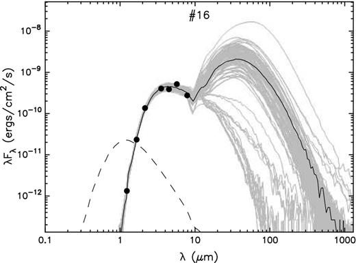
$SED fitting using the online tool of Robitaille et al. (2007) for source #16 (a Class II source) in Table 2. The black dots mark the data points. The solid black curve is the best-fitting model, while the grey curves denote the subsequent good fits for $\chi ^2 - \chi ^2_{{\rm min}}\ {\rm (per data point)} < 3$. The dashed curve is the photosphere (in the presence of interstellar extinction, but absence of circumstellar dust) of the central source for the best-fitting model.$

Figure 3.

SED fitting using the online tool of Robitaille et al. (2007) for source #16 (a Class II source) in Table 2. The black dots mark the data points. The solid black curve is the best-fitting model, while the grey curves denote the subsequent good fits for |$\chi ^2 - \chi ^2_{{\rm min}}\ {\rm (per data point)} < 3$|⁠. The dashed curve is the photosphere (in the presence of interstellar extinction, but absence of circumstellar dust) of the central source for the best-fitting model.

Open in new tab Download slide

It should be noted that the SED results are only representative of the actual values, as an empirically consistent fit might not be the correct fit. A deliberate sampling bias of the huge parameter space, to reduce computational time, could give rise to pseudo-trends in the results. The results are also contingent upon the validity of assumed evolutionary tracks from literature. Most importantly, the models are for individual sources, and could be misleading in cases of stellar multiplicity. The caveats are dealt in detail in Robitaille (2008).

3.3 Luminosity function

The slope of the K_s-band luminosity function (KLF) can serve as an indicator of the age of a stellar cluster (Zinnecker, McCaughrean & Wilking 1993; Lada & Lada 1995; Vig et al. 2014). If we were to assume that the mass function and the mass–luminosity relation for a (coeval) stellar cluster are power laws, i.e. they are of the form |$\mathrm{d}N(\log m_*) \propto m_*^{-\gamma } \mathrm{d}\log m_*$| and |$L_K \propto m_*^B$|⁠, then it can be shown that the slope of the KLF will be of the form:

\begin{equation} \alpha = \gamma /2.5 B \end{equation}

(2)

(Lada, Young & Greene 1993; Megeath 1996). First of all, we try to estimate the KLF slope. We only consider the YSOs here, as opposed to all the observed sources, as they will be much less affected by any field star contamination. Our K-band 100 per cent completeness limit is up to 14 mag, and thus completeness correction was implemented in the (0.5 mag sized) bins after this limit. Thereafter, the (cumulative) KLF of the YSOs was constructed, and is shown in Fig. 4. The fit to the histogram is also shown, and its slope (dlog N/dm_K) in [12,15.5] mag range is calculated to be (α =) 0.35 ± 0.04 (the slope will be same for cumulative and differential KLFs here, see Lada et al. 1993). As for the slope of mass–luminosity relation, if we adopt the value of B = 2 (which can be shown to be the approximate value for O-F main-sequence stars; Lada et al. 1993), then the mass function slope comes out to be (γ =)1.75 ± 0.20 (a value slightly steeper than the Salpeter slope of 1.35).

Figure 4.

The grey dashed histogram shows the cumulative KLF for the YSOs. The black straight line is the fit in [12,15.5] mag range, whose slope is given by α.

Open in new tab Download slide

Alternatively, we could get an estimate of the mass function slope using the SED fitting results. Since most of our sources are of intermediate mass in 2–6 M_⊙ range (see Table 2), we consider only this range to estimate the slope γ. Fig. 5 shows the mass histogram (for the YSOs). Assuming that the star formation is strictly coeval, the mass function slope is given by γ = −(dlog N/dlog m_⋆) (Massey 1998), and thus we calculate γ ∼ 1.59 ± 0.70 for our case. The grey curve in Fig. 5 shows the fitted function for 2–6 M_⊙. This is consistent with γ obtained above. The major source of uncertainty here is the sparse statistics, and thus possible incompleteness in the mass bins.

Figure 5.

Histogram of stellar masses obtained from the SED fitting (Table 2). The grey curve shows the power-law fit in the intermediate mass range.

Open in new tab Download slide

A similar set of values (both α and γ) was found by Balog et al. (2004) for the 1-Myr-old NGC 7538 cluster (distance ∼ 2.65 kpc; Mallick et al. 2014). α also appears consistent with that derived for the Orion molecular clouds (∼0.37–0.38, age ∼ 1 Myr; Lada et al. 1991; Lada & Lada 1995). However, other embedded clusters in literature, such as the NGC 1893 cluster (∼0.34 ± 0.07, distance ∼ 3.25 kpc; Sharma et al. 2007), the Tr 14-16 clusters in Carina nebula (∼0.30–0.37, distance ∼ 2.5 kpc; Sanchawala et al. 2007), and the IRAS 06055+2039 cluster (∼0.43 ± 0.09, distance ∼ 2.6 kpc; Tej et al. 2006) do exhibit slightly larger cluster ages, up to ∼4 Myr. Hence, it appears that 1 Myr should be the lower age limit of the cluster.

3.4 Mass spectrum

In addition to the SED, we also use the J/J − H colour–magnitude diagram (CMD) to get an estimate of the mass range of the YSOs. We avoid using a CMD involving the K-band magnitude as this band is the most affected by the NIR excess flux arising from circumstellar material, which in turn can lead to brightening, and thus erroneous mass estimate, of the sources. Fig. 6 shows the J/J − H CMD for the YSOs with at least J- and H-band detections. The 1-Myr PMS isochrone, along with the 2 Myr isochrone for reference, from Siess, Dufour & Forestini (2000) has been shown on the image. For the 1-Myr PMS isochrone, reddening vectors are shown for 0.1, 1, 2, and 4 M_⊙. As can be seen, all but one of the YSOs for which the SED analysis has been done (marked with blue stars) lie in the mass range ≳ 2 M_⊙, matching well with our SED results. In general, the sources lie in the mass range ∼0.1–4 M_⊙, or, put differently, the observations probe stellar objects up to the 0.1 M_⊙ limit. The (blue star) source at the far-right end of the diagram is the 9.6 M_⊙ high-mass source from SED analysis. The wide variation in the colours of YSOs is probably an indication of variable extinction as well as different evolutionary stages of the sources. Major causes of uncertainty here are: uncertainty in distance estimate which is used to obtain the apparent magnitude (for the isochrones), and unresolved (especially since the source distance of ∼3.6 kpc is much larger than most of the previously studied clusters) binarity. Additionally, it should be kept in mind that, in general, a particular PMS model will introduce its own systematic error.

Figure 6.

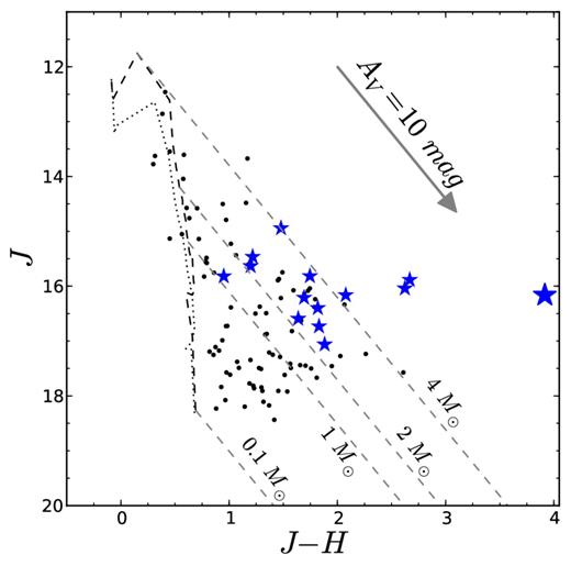
J/J − H CMD for the YSOs with at least J- and H-band detections. The dashed and dotted black curves plot the 1- and 2-Myr PMS isochrones, respectively, from Siess et al. (2000). The reddening vectors (parallel grey dashed lines) for the 1 Myr isochrone are drawn at 0.1, 1, 2, and 4 M_⊙. The blue star symbols are the sources for which SED analysis was done.

Open in new tab Download slide

4 MORPHOLOGY OF THE REGION

4.1 Cluster analysis and extinction mapping

Fig. 7 shows the Spitzer 8.0 μm image with overlaid surface density contours (in cyan) as well as visual extinction contours (in blue). The high-mass source in this region (see Section 3.2), as well as the mm and MSX peaks from Molinari et al. (2008, 16148-5011 MM 1 and 16148-5011 A from their tables 2 and 3, respectively) have also been marked on the image. The marked mm peak is almost coincident with the (mm) peak from Beltrán et al. (2006, 16148-5011 Clump 2 from their table 2). The surface density and extinction contours were calculated as follows. The surface density analysis was carried out using the nearest-neighbour (NN) method (Casertano & Hut 1985) to discern the YSO clusterings in the region. We chose 20 NN, similar to Schmeja, Kumar & Ferreira (2008), Schmeja (2011), and Mallick et al. (2013). The extinction in the region was estimated by constructing the extinction map with the help of the NIR photometric data. We use the NIR CCD (see Fig. 2c) for this purpose. In this NIR CCD, the ‘F’ region mostly contains the main-sequence field sources along with a few probable Class III sources. Since these are sources which have almost lost their circumstellar material, any extinction they exhibit will come from interstellar – rather than circumstellar – material. The sources from this ‘F’ region, which were not identified as a YSO in Section 3.1, were therefore selected. Subsequently, we used a method similar to the Near-IR-Colour-Excess method of Lada et al. (1994), but here the (H − K) colour excess was estimated by dereddening the sources – along the reddening vector – to the low-mass end (turnover onwards) of the dwarf locus (which was approximated as a straight line). A_V was then calculated using the reddening laws of Cohen et al. (1981). After we obtained the visual extinction A_V for each source, an extinction map of the region was made by using the NN method, where the extinction at each grid point on the map is the median (because median rejects outliers) of A_V of 20 NN. It is possible that the extinction could be slightly underestimated because, due to the large distance to this region, a significant fraction of the detected sources could be foreground sources, especially towards the centre of the nebula.

Spitzer 8.0 μm image of the region with overlaid surface density contours (at 5, 5.75, 6, 7, 7.5, and 8 YSOs pc−2) in cyan, and visual extinction contours (at AV = 4, 4.5, 5, 6, and 6.5 mag) in blue. Green plus symbol marks the IRAS catalogue position of IRAS 16148−5011, green cross the high-mass source (#16 from Table 2), while the diamond and box symbols mark the mm and MSX peaks, respectively, from Molinari et al. (2008).

Figure 7.

Spitzer 8.0 μm image of the region with overlaid surface density contours (at 5, 5.75, 6, 7, 7.5, and 8 YSOs pc⁻²) in cyan, and visual extinction contours (at A_V = 4, 4.5, 5, 6, and 6.5 mag) in blue. Green plus symbol marks the IRAS catalogue position of IRAS 16148−5011, green cross the high-mass source (#16 from Table 2), while the diamond and box symbols mark the mm and MSX peaks, respectively, from Molinari et al. (2008).

Open in new tab Download slide

In Fig. 7, the surface density contours are drawn at 5, 5.75, 6, 7, 7.5, and 8 YSOs pc⁻², while the extinction contours have been drawn at A_V = 4, 4.5, 5, 6, and 6.5 mag levels. As can be seen on the image, both the surface density as well as extinction contours are in the southern portion of the nebular emission and appear to be along the sharp boundary of the nebula. The highest surface density contour levels coincide with the highest extinction levels. Though we would have expected to see high interstellar extinction along the main body of the nebula, this is not so possibly because the NIR observations are not deep enough to detect stars from behind the nebula and thus the extinction of the nebula should be higher than the highest extinction contour level here (it is later estimated to be A_V > 20 mag; see Section 4.4) It should also be noted that the cluster detected here is in the southern part of the nebula also coincident with extended radio continuum emission (see Section 4.2).

4.2 Radio morphology

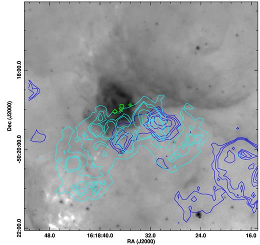
Fig. 8 shows a Spitzer 8.0 μm image of the region with overlaid 843 MHz contours from MGPS and 1280 MHz contours from GMRT. Rest of the objects marked are same as in Fig. 7. The central core appears to be a compact H ii region, near whose peak lie the mm peak and the high-mass source. The 843 MHz contours show extended emission in addition to the central compact region. The extended emission is only in the southern part and none in the northern part of the compact H ii region, indicating the presence of dense molecular cloud in the northern part which is not ionized to the same extent as the southern region. The background 8.0 μm image also shows the diffuse nebular emission in the north. Using the aips task JMFIT, the compact cores at both the frequencies were fitted with a Gaussian model to determine the source sizes and the fluxes. The obtained results are given in Table 3. The beam-deconvolved source size for MGPS 843 MHz is found to be much larger in area than that for 1280 MHz. The larger integrated flux density for 843 MHz could be because of this. Fig. 9 shows the maximum resolution image of the region which could be obtained at 1280 MHz (∼7 arcsec × 2 arcsec), overlaid on the Herschel 70 μm image. This contours show multiple peaks which is probably indicative of the clumpy nature of the ionized matter in the region. These peaks are mostly coincident with large 70 μm emission, which is to be expected as 70 μm also traces the thermal dust emission.

Figure 8.

Spitzer 8.0 μm image of the region with overlaid 1280-MHz contours (at 3σ, 4σ, 5σ, 7σ, 10σ, 12σ, 15σ, 20σ, and 22 σ, where σ ∼ 8.85 mJy; resolution ∼56 arcsec × 35 arcsec) in cyan and 843 MHz contours (at 5σ, 7σ, 10σ, 15σ, 20σ, 30σ, 40σ, and 50 σ, where σ ∼ 5.57 mJy; resolution ∼ 56 arcsec × 43 arcsec) in blue. The symbols are same as for Fig. 7.

Open in new tab Download slide

Figure 9.

The colour map Herschel 70 μm image with overlaid 1280 MHz contours at 3σ, 4σ, 5σ, 7σ, 11σ, 13σ, 15σ, 17σ, 19σ, 20σ, and 21 σ (where σ ∼ 0.4 mJy). The contours are from the maximum resolution (7 arcsec × 2 arcsec) radio continuum image that could be constructed at 1280 MHz. The symbols are same as Fig. 7.

Open in new tab Download slide

Table 3.

Open in new tab

Fitting results for compact H ii region.

	1280 MHz	843 MHz
2D Gaussian fit
size	60.30 arcsec × 39.71 arcsec	69.41 arcsec × 76.17 arcsec
Beam-deconvolved
source size	23.35 arcsec × 18.31 arcsec	51.25 arcsec × 54.97 arcsec
Position Angle (deg)	160.1	128.2
Peak flux
Density (mJy beam⁻¹)	204 ± 9	258 ± 5
Integrated flux
density (mJy)	252 ± 18	552 ± 16

	1280 MHz	843 MHz
2D Gaussian fit
size	60.30 arcsec × 39.71 arcsec	69.41 arcsec × 76.17 arcsec
Beam-deconvolved
source size	23.35 arcsec × 18.31 arcsec	51.25 arcsec × 54.97 arcsec
Position Angle (deg)	160.1	128.2
Peak flux
Density (mJy beam⁻¹)	204 ± 9	258 ± 5
Integrated flux
density (mJy)	252 ± 18	552 ± 16

Table 3.

Open in new tab

Fitting results for compact H ii region.

	1280 MHz	843 MHz
2D Gaussian fit
size	60.30 arcsec × 39.71 arcsec	69.41 arcsec × 76.17 arcsec
Beam-deconvolved
source size	23.35 arcsec × 18.31 arcsec	51.25 arcsec × 54.97 arcsec
Position Angle (deg)	160.1	128.2
Peak flux
Density (mJy beam⁻¹)	204 ± 9	258 ± 5
Integrated flux
density (mJy)	252 ± 18	552 ± 16

	1280 MHz	843 MHz
2D Gaussian fit
size	60.30 arcsec × 39.71 arcsec	69.41 arcsec × 76.17 arcsec
Beam-deconvolved
source size	23.35 arcsec × 18.31 arcsec	51.25 arcsec × 54.97 arcsec
Position Angle (deg)	160.1	128.2
Peak flux
Density (mJy beam⁻¹)	204 ± 9	258 ± 5
Integrated flux
density (mJy)	252 ± 18	552 ± 16

We tried to estimate the physical parameters of the region, using the lower resolution images, as follows. The Lyman continuum luminosity (in photons s⁻¹) required to generate the observed flux density was determined using the following formula (adapted from Kurtz, Churchwell & Wood 1994, see their equations 1 and 3):

\begin{eqnarray} S_{*} \ge \left(\frac{7.59\times 10^{48}}{a(\nu , T_{\rm e})}\right) \left(\frac{S_{\nu }}{Jy}\right) \left(\frac{T_{{\rm e}}}{K}\right)^{-0.5} \left(\frac{D}{{\rm kpc}}\right)^{2} \left(\frac{\nu }{{\rm GHz}}\right)^{0.1},\nonumber\\ \end{eqnarray}

(3)

where S_ν is the integrated flux density in Jy, D is the distance in kiloparsec, T_e is the electron temperature, a(ν, T_e) is the correction factor, and ν is the frequency in GHz at which the luminosity is to be calculated. The dynamical age of the H ii region (t) can be solved for by using the following equation from Spitzer (1978):

\begin{equation} R(t)=R_{{\rm s}}\left(1+\frac{7c_{{\rm II}}t}{4R_{{\rm s}}}\right)^{4/7}, \end{equation}

(4)

where R(t) is the radius of the H ii region at time t, c_II is the speed of sound in H ii region (11 × 10⁵ cm s⁻¹; Stahler & Palla 2005), and R_s is the Strömgren radius. The Strömgren radius (R_s, in cm) is given by (Strömgren 1939)

\begin{equation} R_{{\rm s}}=\left(\frac{3S_{*}}{4\pi n_{o}^{2}\beta _{2}}\right)^{1/3}, \end{equation}

(5)

where n_o is the initial ambient density (in cm⁻³), and β₂ is the total recombination coefficient to the first excited state of hydrogen. For our calculation, we assume a typical value of 10 000 K for T_e (which will imply a value of 0.99 for the correction factor ‘a’; see table 6 of Mezger & Henderson 1967), and the corresponding β₂ of 2.6 × 10⁻¹³ cm³ s⁻¹ (Stahler & Palla 2005). For n_o, we use the value of 4.8 × 10⁴ cm⁻³ from Beltrán et al. (2006). R(t) is taken as the geometric mean of fitted Gaussian source sizes from Table 3. Using these formulae and the 1280 MHz data, we calculated S_* and t as ∼10^47.41 photons s⁻¹ and ∼0.3 Myr, respectively. If we were to use the 843-MHz flux density data point, then S_* and t come out to be ∼10^47.73 photons s⁻¹ and ∼0.5 Myr, respectively. Assuming Zero Age Main Sequence (ZAMS), a comparison of log S_* with the tabulated values from Panagia (1973) shows that a spectral type of B0-O9.5 corresponds to this luminosity. Recent calibrations, like Martins, Schaerer & Hillier (2005), also suggest a (luminosity class V) spectral type of ∼O9.5. So, it seems that the spectral type of the source ionizing the region (assuming a single source) has to be earlier than B0-O9.5 for the ionization in the nebula to be sustained, since there can be absorption of ionizing photons by dust in the region which is often significant (Arthur et al. 2004). The dynamical age is approximately of the order of a few tenths of Myr.

We also try to fit to our data the free–free emission model of Mezger & Henderson (1967), according to which (adapted from Mezger, Schraml & Terzian 1967)

\begin{equation} S_{\nu }/\Omega =3.07\times 10^{-2}T_{{\rm e}}\nu ^{2} (1-{\rm e}^{-\tau (\nu )}) \end{equation}

(6)

\begin{equation} \tau (\nu )=1.643\times 10^{5}a(\nu , T_{\rm e})T_{{\rm e}}^{-1.35}\nu ^{-2.1}n_{{\rm e}}^{2}l, \end{equation}

(7)

where, S_ν is the integrated flux density (in Jy), ν is the frequency (in MHz), n_e is the electron density in cm⁻³, l is the extent of the ionized region in pc, τ is the optical depth, and Ω is the solid angle subtended by the source (in steradians). |$n_{{\rm e}}^{2}l$| measures the optical depth in the medium (in cm⁻⁶ pc), and is called the emission measure. Taking Ω as (1.133 × θ_major × θ_minor), and the two data points, we fit the above equation using non-linear regression keeping |$n_{\rm e}^2 l$| – the emission measure – as a free parameter. The fit is shown in Fig. 10. The emission measure is thus determined to be ∼4.00 ± 0.09 × 10⁴ cm⁻⁶ pc. Since most of the central radio emission is confined within a circle of 120 arcsec diameter, we can assume it to be the extent of the H ii region (∼2.1 pc), and thus the electron density (n_e) turns out to be ∼138 cm⁻³. Further, using the formula from Mezger et al. (1967, equation A.5), we calculate the total mass of ionized hydrogen (M|$_{\rm H\small {\,ii}}$|⁠) to be ∼16.4 M_⊙. These low values of n_e and M|$_{\rm H\small {\,ii}}$|⁠, as well as the extent, would suggest that this region might be slightly more evolved than a compact H ii region (Kurtz & Franco 2002).

Figure 10.

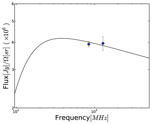
The fitted free–free emission model for the H ii region. The data points at 843 and 1280 MHz have been marked with solid circles.

Open in new tab Download slide

4.3 Central region

Fig. 11 shows the central 1 arcmin × 1 arcmin region of IRAS 16148−5011 in the NIR J and K_s bands, IRAC 3.6, 4.5, and 8.0 μm bands, and the MIPS 24 μm band. The IRAC 3.6 and 8.0 μm bands, besides the continuum emission, also encompass the weak polycyclic aromatic hydrocarbon (PAH) emission feature at 3.3 μm, and strong PAH features at 7.7 and 8.6 μm. The 4.5 μm band does not contain any PAH features, but does contain shocked molecular gas emission from H₂(v = 0 − 0) S(9, 10, 11) and CO(v = 1 − 0). 24-μm emission is mainly the thermal continuum emission from the hot dust (Watson et al. 2008; Churchwell et al. 2009).

Figure 11.

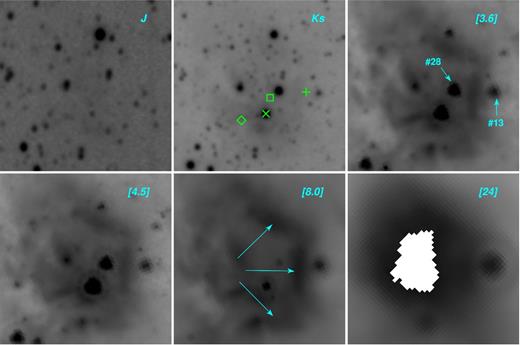
1 arcmin × 1 arcmin central region of IRAS 16148−5011. The images (left-to-right, top-to-bottom) are J, K_s, 3.6, 4.5, 8.0, and 24 μm. North is up and east is to the left. The symbols on the K_s band image are same as Fig. 7 (green cross is #16 from Table 2). The numbered sources on the 3.6 μm image are from Table 2. The cyan arrows on the 8.0 μm image mark the ‘ring-like’ morphology. The white patch on the 24 μm image is the saturated region.

Open in new tab Download slide

The K_S band image has been marked with, among others, the high-mass source detected (green cross, #16 in Table 2) and the MSX peak from Molinari et al. (2008, ‘IRAS 16148−5011 A’) (green box). The marked high-mass source is of ∼B2–B3 spectral type (as per tabulated values from Stahler & Palla 2005, see their table 1.1), while the radio flux suggests an ionizing star of type ≥ B0-O9.5. In addition, Molinari et al. (2008), using SED modelling (assuming an embedded ZAMS source) and the MSX flux values, have estimated the spectral type of ‘IRAS 16148−5011 A’ source as O8. Therefore, it appears that there could be further embedded high-mass source(s) in this region, in addition to those seen in NIR and MIR, for the values to be consistent. It is possible that the cores seen by radio contours in Fig. 9 could be hosting such high-mass source(s) and contributing to the radio luminosity.

The other sources associated with this central part of the nebula have been marked on the 3.6 μm image (#13 and #28 from Table 2, Section 3.2). The source #13 appears to be a highly embedded intermediate-mass young source (∼6.17 M_⊙, ∼a few 10⁴ yr; see Section 3.2), even visible at 24 μm. Source #28 appears to be a much older and evolved source (∼8.48 M_⊙, ∼a few 10⁶ yr), possibly shrouded in the surrounding nebulosity (interstellar extinction of A_V ∼ 18.38 mag), leading to a lack of detection in the J band (though it is the second brightest source after the 9.6 M_⊙ – #16 from Table 2 – source in the central region in K_s band). The radio continuum emission contribution from this source will be much lower, hardly making a difference even when taken in combination with the emission from the high-mass source, and thus will not affect the inferences regarding radio emission above.

For H ii regions, the PAH emissions serve as useful diagnostic tools as they are characteristic of photodissociation regions (PDRs). As a high-mass star ionizes its natal medium, the UV radiation destroys the PAH in its surroundings. However, at the boundary of the H ii region produced, the UV intensity falls off, and a PDR is formed where the PAH's are merely highly excited, leading to strong emission (Povich et al. 2007). The PDR is supposed to be the transition region between the ionized and neutral matter. This usually results in a ‘bubble’ morphology, where H ii regions surrounded by ring-like PAH emission are seen (Churchwell et al. 2006). A similar morphology can be seen in the 3.6 and the 8.0 μm image in Fig. 11. A ‘semiring’ in the western half of the image is seen (marked by cyan arrows on the 8.0-μm image). We note that this feature is also faintly seen in the 4.5 μm image, though this could just be continuum emission. That this ring-like feature does not appear symmetric (i.e. there is no clear eastern ‘semi-ring’, though faint indications are seen) could possibly be due to eastern denser and/or non-homogeneous molecular cloud, or projection effects. Volk et al. (1991), on the basis of low-resolution spectra, had classified IRAS 16148−5011 as a PAH source. Bulk of the radio emission (see Fig. 8), as well as the 24 μm emission from hot dust, is confined within this ring-like feature as expected (Watson et al. 2008). Some of the emission from this ring-like structure could also be due to swept-up material by the expanding ionization front of the H ii region.

4.4 Herschel results

Thermal emission from cold dust lies in the FIR wavelength range, and thus its analysis can be used to obtain the physical parameters like dust temperature and column density of a region (Battersby et al. 2011; Launhardt et al. 2013). This was carried out by the SED modelling of the thermal dust emission, whose Rayleigh–Jeans regime is covered by the Herschel FIR bands (160–500 μm), using the following order of steps.

First of all, the surface brightness unit for all the images was converted to Jy pixel⁻¹. Since the PACS image is already in Jy pixel⁻¹, this step was only required for the SPIRE images (whose units are in MJy sr⁻¹), and was carried out using the pixel scales for the respective SPIRE bands. Next, the 160–350 μm images were convolved to the resolution of the 500 μm image (∼36 arcsec, lowest among all images) using the convolution kernels of Aniano et al. (2011), and regridded to a pixel scale of 14 arcsec (same as 500 μm image). Using these final reworked images with same resolution and pixel scale, a background flux level, I_bg, was determined from a ‘smooth’ (i.e. no abrupt clumpy regions) and relatively ‘dark’ patch of the sky. The distribution of individual pixel values in the dark patch of the sky, for each of the bands, was fitted with a Gaussian iteratively, rejecting the pixel values outside ± 2σ in each iteration, till the fit converged. The same patch of the sky was used for each band. The background flux level, I_bg, was thus determined as 0.29, 2.67, 1.27, and 0.45 Jy pixel⁻¹ for the 160, 250, 350, and 500 μm images, respectively. We note that the 70 μm image, though available, was not used here as the optically thin assumption might not hold true at this wavelength (Lombardi et al. 2014).

Modified blackbody fitting was subsequently carried out on a pixel-by-pixel basis using the following formulation (Battersby et al. 2011; Sadavoy et al. 2012; Nielbock et al. 2012; Launhardt et al. 2013):

\begin{equation} S_{\nu }(\nu ) - I_{{\rm bg}}(\nu ) = B_{\nu }(\nu , T_{\rm d}) \Omega (1-{\rm e}^{-\tau (\nu )}), \end{equation}

(8)

with

\begin{equation} \tau (\nu ) = \mu _{{\rm H}_2} m_{\rm H} \kappa _{\nu } N(H_2), \end{equation}

(9)

where, ν is the frequency, S_ν(ν) is the observed flux density, I_bg(ν) is the background flux in that particular band (estimated above), B_ν(ν, T_d) is the Planck function, T_d is the dust temperature, Ω is the solid angle (in steradians) from where the flux is obtained (just the solid angle subtended by a 14 arcsec × 14 arcsec pixel here), τ(ν) is the optical depth, |$\mu _{{\rm H}_2}$| is the mean molecular weight (adopted as 2.8 here), m_H is the mass of hydrogen, κ_ν is the dust opacity, and N(H₂) is the column density. For opacity, we adopt a functional form of κ_ν = 0.1 (ν/1000 GHz)^β cm² g⁻¹, with β = 2 (see Hildebrand 1983, Beckwith et al. 1990, André et al. 2010). For each pixel, equation (8) was fitted using the four data points, keeping T_d and N(H₂) as free parameters. Pixels for which the fit did not converge, or the error was larger than 10 per cent, had their values taken as the median of eight immediate-neighbour pixels. The final obtained temperature and column density maps of the wider region (to clearly discern the morphological features) surrounding IRAS 16148−5011 are shown in Fig. 12.

Figure 12.

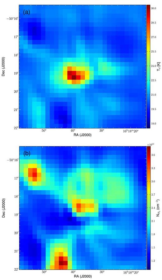
(a) Dust temperature map, and (b) column density map of the region around IRAS 16148−5011, derived using the SED fitting to the thermal dust emission.

Open in new tab Download slide

From the temperature (Fig. 12a) and column density (Fig. 12b) maps, we obtain the peak values as ∼30 K and 3.3 × 10²² cm⁻², respectively, for IRAS 16148−5011. Fontani et al. (2005) provide a temperature of 38 K (using greybody fit with 60 μm, 100 μm, and 1.2 mm data), and a (beam-averaged) column density of 3 × 10²³ cm⁻² (using C¹⁷O molecular line observations) for IRAS 16148−5011. Here our peak temperature is about 20 per cent lower, and the column density estimate an order of magnitude smaller. The difference in temperature seems to be due to their fitting limitations owing to sparse data points, as well as the fact that the 60 μm emission might not be optically thin. It should be noted, however, that the dust temperature distribution from Fontani et al. (2005, for their analysed catalogue of IRAS sources) peaks at ∼30 K. Column density disparity can probably be explained by the dependence of Fontani et al. (2005) on the molecular abundance of the rare C¹⁷O, whose value can have wide variations (Redman et al. 2002; Walsh et al. 2010).

The column density map (Fig. 12b) displays three peaks – the central IRAS 16148−5011 object, a peak to its north-east, and a peak to its south. These north-east and south peaks appear to be associated with cold clumps, as is evident from the temperature map which shows T_d < 20 K at their positions. The column density map shows that all the peaks appear to be connected by weak filamentary features, similar to previous results for myriad regions (see André 2013, and references therein). For the central IRAS 16148−5011 object, we estimated the associated clump dimensions, using the ‘clumpfind’ software (Williams, de Geus & Blitz 1994), to be ∼62 arcsec × 46 arcsec (i.e. 1.1 pc × 0.8 pc at 3.6 kpc). Due to the low resolution of the column density image generated here, it does not appear possible to resolve further sub-clumps. The mass of the clump can be estimated by

\begin{eqnarray} M_{{\rm clump}} &=& \mu _{{\rm H}_2}\ m_{{\rm H}}\ \Sigma \ N({\rm H}_2)\ Area_{{\rm pixel}} \end{eqnarray}

(10)

\begin{eqnarray} = \mu _{{\rm H}_2}\ m_{{\rm H}}\ Area_{{\rm pixel}}\ \Sigma \ N({\rm H}_2), \end{eqnarray}

(11)

i.e. calculating the mass in each pixel and then summing over all the pixels which constitute the clump. Using the Σ N(H₂) returned by the ‘clumpfind’ software, the total clump mass was calculated to be ∼1023 M_⊙.

Another noticeable feature in this map is that the immediate northern vicinity of the central region exhibits higher column density than the immediate southern portion. This suggests dense nebula in the northern part, affirming the inference also drawn from extinction and cluster analysis in Section 4.1 (also see Fig. 7). This is also consonant with the fact that the dense nebular emission is in the northern part, with no extended radio emission seen there (unlike in the southern part). To get an estimate of the visual extinction in this northern part, we use the relation 〈N(H₂)/A_V〉 = 0.94 × 10²¹ molecules cm⁻¹ mag⁻¹ (adapted from Bohlin, Savage & Drake 1978, assuming a total-to-selective extinction ratio R_V = 3.1, and that the gas is in molecular form). Now, typical N(H₂) seen here is ≳2 × 10²² cm⁻³, which implies an A_V > 20 mag. This high value of A_V is probably the reason why very few YSOs are associated with this northern nebular emission (see Fig. 7). If the value of R_V were to be larger, as has been conjectured for dense environments, then it will lead to an increase in A_V.

5 DISCUSSION

The IRAS 16148−5011 region appears to be hosting an infrared cluster containing high-mass star(s) embedded in the nebula, and could serve as a future template to study the high-mass star formation process. Age estimates for any cluster are usually plagued with uncertainties (see Lada & Lada 2003, for a discussion), and various proxies are often used to ascertain the evolutionary stage of a cluster. One such is the ratio of Class II to Class I sources (as Class II sources are older; Schmeja, Klessen & Froebrich 2005; Gutermuth et al. 2009; Beerer et al. 2010). We have detected 133 Class II and 7 Class I sources in this region. However, here it seems that the large ratio (19) could be because Class I sources are deeply embedded and their detection is affected by large nebular extinction, though varying ratio values have been estimated for other clusters (Gutermuth et al. 2009).

The two brightest (NIR) sources in the central region appear to be high-mass (see Section 4.3) with indications of further embedded high-mass sources. Also in literature, Beltrán et al. (2006) report two clumps within 90 arcsec of the IRAS 16148−5011 IRAS catalogue position – ‘16148-5011 Clump 2’ (206 M_⊙) and ‘16148-5011 Clump 3’ (42 M_⊙) – detected using 1.2 mm emission and a dust temperature of 30 K. While ‘Clump 2’, is almost coincident with the ‘16148-5011 MM 1’ peak from Molinari et al. (2008, marked with a diamond symbol on Fig. 11), ‘Clump 3’ coordinates are same as the IRAS 16148−5011's IRAS catalogue coordinates (green plus in Fig. 11). The presence of these massive clumps could also point towards ongoing high-mass star formation in the region.

Though this part of the sky also harbours other IRAS sources (Karnik et al. 2001), IRAS 16148−5011 does not appear to be a part of any larger star-forming complex as such, but it seems to be connected to other clumps via filaments (similar to the hub-filament morphology of Myers 2009). The high-mass stellar cluster formation in the associated molecular cloud appears to be spontaneous. However, along the rather sharp southern boundary of the molecular cloud, the results from cluster analysis show a stellar sub-cluster forming (Fig. 7), which could partly be due to the triggering by the expanding ionization front of the H ii region.

6 CONCLUSIONS

The main conclusions of this paper, resulting from a multiwavelength study involving NIR, MIR, FIR, and radio continuum data, are as follows.

7 Class I and 133 Class II YSOs are identified using a combination of NIR and MIR data. A 9.6-M_⊙ high-mass source is found to be associated with the central nebula.
Low-frequency radio emission reveals a compact H ii region, with extended emission in the southern part. Lyman continuum photon luminosity calculation gives B0-O9.5 as the lower limit for the spectral type of the ionizing source (assuming single source). The dynamical age of the H ii region is in 0.3–0.5 Myr range. SED modelling of the free–free emission yields an electron density of 138 cm⁻³. The mass of the ionized hydrogen is calculated to be ∼16.4 M_⊙. The high-resolution 7 arcsec × 2 arcsec contour map shows clumpy ionized gas in the region.
The central nebular region shows a ring-like PAH emission feature near the borders of the compact H ii region, tracing the PDR. There appear to be three NIR- and MIR-visible central sources, of masses ∼6.2, 9.60, and 8.5 M_⊙. Based on the incongruence between the total radio flux from these sources and the flux obtained from radio observations, and literature estimates of an early-type star using MIR SED fitting, it is possible that there could be high-mass embedded source(s) present in this region.
Dust temperature and column density maps are obtained using SED modelling of the thermal dust emission. The peak temperature and column density values are 30 K and 3.3 × 10²² cm⁻², respectively, for IRAS 16148−5011. The column density map reveals that the immediate northern vicinity of IRAS 16148−5011, which contains the nebular emission seen prominently at MIR wavelengths, has a large extinction of A_V > 20 mag. This map also shows that weak filamentary structures join IRAS 16148−5011 to nearby cold clumps. The size and mass of the clump associated with IRAS 16148−5011 is estimated to be ∼1.1 pc × 0.8 pc (at 3.6 kpc) and ∼1023 M_⊙, respectively.

Future observations of individual objects in spectral lines, deeper IR data to get a full stellar census up to below brown-dwarf limit, further molecular line observations which probe high column densities will help put the star formation scenario on a firm footing and help study high-mass star formation.

We thank the anonymous referee for a thorough reading of the manuscript, and for the useful comments and suggestions which helped improve its scientific content. The authors thank the staff of IRSF in South Africa, a joint partnership between S.A.A.O and Nagoya University of Japan; and GMRT managed by National Center for Radio Astrophysics of the Tata Institute of Fundamental Research (TIFR) for their assistance and support during observations. DKO was supported by the National Astronomical Observatory of Japan (NAOJ), Mitaka, through a fellowship, during which a part of this work was done.

1

see http://rms.leeds.ac.uk/.

2

http://gmrt.ncra.tifr.res.in/gmrt_hpage/Users/Help/help.html

3

http://www.physics.usyd.edu.au/sifa/Main/MGPS1

4

The MOST is operated by the University of Sydney with support from the Australian Research Council and the Science Foundation for Physics within the University of Sydney.

5

This research has made use of the NASA/ IPAC Infrared Science Archive, which is operated by the Jet Propulsion Laboratory, California Institute of Technology, under contract with the National Aeronautics and Space Administration.

6

http://www.cosmos.esa.int/web/herschel/science-archive

7

http://www.cosmos.esa.int/web/herschel/data-products-overview

REFERENCES

André

P.

,

2013

Invited Discourse at the IAU XXVIII General Assembly (Beijing, Aug. 2012), preprint (arXiv:1309.7762)

André

P.

et al. ,

A&A

,

2010

, vol.

518

pg.

L102

Crossref

Search ADS

Aniano

G.

Draine

B. T.

Gordon

K. D.

Sandstrom

K.

,

PASP

,

2011

, vol.

123

pg.

1218

Crossref

Search ADS

Arthur

S. J.

Kurtz

S. E.

Franco

J.

Albarrán

M. Y.

,

ApJ

,

2004

, vol.

608

pg.

282

Crossref

Search ADS

Balog

Z.

Kenyon

S. J.

Lada

E. A.

Barsony

M.

Vinkó

J.

Gáspaŕ

A.

,

AJ

,

2004

, vol.

128

pg.

2942

Crossref

Search ADS

Battersby

C.

et al. ,

A&A

,

2011

, vol.

535

pg.

A128

Crossref

Search ADS

Beckwith

S. V. W.

Sargent

A. I.

Chini

R. S.

Guesten

R.

,

AJ

,

1990

, vol.

99

pg.

924

Crossref

Search ADS

Beerer

I. M.

et al. ,

ApJ

,

2010

, vol.

720

pg.

679

Crossref

Search ADS

Beltrán

M. T.

Brand

J.

Cesaroni

R.

Fontani

F.

Pezzuto

S.

Testi

L.

Molinari

S.

,

A&A

,

2006

, vol.

447

pg.

221

Crossref

Search ADS

Benjamin

R. A.

et al. ,

PASP

,

2003

, vol.

115

pg.

953

Crossref

Search ADS

Bessell

M. S.

Brett

J. M.

,

PASP

,

1988

, vol.

100

pg.

1134

Crossref

Search ADS

Bohlin

R. C.

Savage

B. D.

Drake

J. F.

,

ApJ

,

1978

, vol.

224

pg.

132

Crossref

Search ADS

Cantalupo

C. M.

Borrill

J. D.

Jaffe

A. H.

Kisner

T. S.

Stompor

R.

,

ApJS

,

2010

, vol.

187

pg.

212

Crossref

Search ADS

Carpenter

J. M.

,

AJ

,

2001

, vol.

121

pg.

2851

Crossref

Search ADS

Casertano

S.

Hut

P.

,

ApJ

,

1985

, vol.

298

pg.

80

Crossref

Search ADS

Chan

S. J.

Henning

T.

Schreyer

K.

,

A&AS

,

1996

, vol.

115

pg.

285

Chavarría

L. A.

Allen

L. E.

Hora

J. L.

Brunt

C. M.

Fazio

G. G.

,

ApJ

,

2008

, vol.

682

pg.

445

Crossref

Search ADS

Churchwell

E.

et al. ,

ApJ

,

2006

, vol.

649

pg.

759

Crossref

Search ADS

Churchwell

E.

et al. ,

PASP

,

2009

, vol.

121

pg.

213

Crossref

Search ADS

Cohen

J. G.

Persson

S. E.

Elias

J. H.

Frogel

J. A.

,

ApJ

,

1981

, vol.

249

pg.

481

Crossref

Search ADS

Dutra

C. M.

Bica

E.

Soares

J.

Barbuy

B.

,

A&A

,

2003

, vol.

400

pg.

533

Crossref

Search ADS

Flaherty

K. M.

Pipher

J. L.

Megeath

S. T.

Winston

E. M.

Gutermuth

R. A.

Muzerolle

J.

Allen

L. E.

Fazio

G. G.

,

ApJ

,

2007

, vol.

663

pg.

1069

Crossref

Search ADS

Fontani

F.

Beltrán

M. T.

Brand

J.

Cesaroni

R.

Testi

L.

Molinari

S.

Walmsley

C. M.

,

A&A

,

2005

, vol.

432

pg.

921

Crossref

Search ADS

Grave

J. M. C.

Kumar

M. S. N.

,

A&A

,

2009

, vol.

498

pg.

147

Crossref

Search ADS

Green

A. J.

Cram

L. E.

Large

M. I.

Ye

T.

,

ApJS

,

1999

, vol.

122

pg.

207

Crossref

Search ADS

Griffin

M. J.

et al. ,

A&A

,

2010

, vol.

518

pg.

L3

Crossref

Search ADS

Gutermuth

R. A.

Megeath

S. T.

Myers

P. C.

Allen

L. E.

Pipher

J. L.

Fazio

G. G.

,

ApJS, 184, 18; erratum, 2010, ApJS

,

2009

, vol.

189

pg.

352

Haslam

C. G. T.

Salter

C. J.

Stoffel

H.

Wilson

W. E.

,

A&AS

,

1982

, vol.

47

pg.

1

Haynes

R. F.

Caswell

J. L.

Simons

L. W. J.

,

Aust. J. Phys.

,

1979

, vol.

48

pg.

1

Hildebrand

R. H.

,

QJRAS

,

1983

, vol.

24

pg.

267

Hillenbrand

L. A.

Strom

S. E.

Vrba

F. J.

Keene

J.

,

ApJ

,

1992

, vol.

397

pg.

613

Crossref

Search ADS

Karnik

A. D.

Ghosh

S. K.

Rengarajan

T. N.

Verma

R. P.

,

MNRAS

,

2001

, vol.

326

pg.

293

Crossref

Search ADS

Kurtz

S.

Franco

J.

,

Rev. Mex. Astron. Astrofis.

,

2002

, vol.

12

pg.

16

Kurtz

S.

Churchwell

E.

Wood

D. O. S.

,

ApJS

,

1994

, vol.

91

pg.

659

Crossref

Search ADS

Lada

C. J.

Peimbert

M.

Jugaku

J.

,

Proc. IAU Symp. 115, Star Forming Regions

,

1987

Dordrecht

Reidel

pg.

1

Google Scholar

Google Preview

OpenURL Placeholder Text

WorldCat

Lada

C. J.

Adams

F. C.

,

ApJ

,

1992

, vol.

393

pg.

278

Crossref

Search ADS

Lada

E. A.

Lada

C. J.

,

AJ

,

1995

, vol.

109

pg.

1682

Crossref

Search ADS

Lada

C. J.

Lada

E. A.

,

ARA&A

,

2003

, vol.

41

pg.

57

Crossref

Search ADS

Lada

E. A.

Depoy

D. L.

Evans

N. J.

II

Gatley

I.

,

ApJ

,

1991

, vol.

371

pg.

171

Crossref

Search ADS

Lada

C. J.

Young

E. T.

Greene

T. P.

,

ApJ

,

1993

, vol.

408

pg.

471

Crossref

Search ADS

Lada

C. J.

Lada

E. A.

Clemens

D. P.

Bally

J.

,

ApJ

,

1994

, vol.

429

pg.

694

Crossref

Search ADS

Launhardt

R.

et al. ,

A&A

,

2013

, vol.

551

pg.

A98

Crossref

Search ADS

Lombardi

M.

Bouy

H.

Alves

J.

Lada

C. J.

,

A&A, 566, A45; erratum, 2014, A&A

,

2014

, vol.

568

pg.

1

Lumsden

S. L.

Hoare

M. G.

Urquhart

J. S.

Oudmaijer

R. D.

Davies

B.

Mottram

J. C.

Cooper

H. D. B.

Moore

T. J. T.

,

ApJS

,

2013

, vol.

208

pg.

11

Crossref

Search ADS

MacLeod

G. C.

van der Walt

D. J.

North

A.

Gaylard

M. J.

Galt

J. A.

Moriarty-Schieven

G. H.

,

AJ

,

1998

, vol.

116

pg.

2936

Crossref

Search ADS

Mallick

K. K.

Kumar

M. S. N.

Ojha

D. K.

Bachiller

R.

Samal

M. R.

Pirogov

L.

,

ApJ

,

2013

, vol.

779

pg.

113

Crossref

Search ADS

Mallick

K. K.

et al. ,

MNRAS

,

2014

, vol.

443

pg.

3218

Crossref

Search ADS

Martins

F.

Schaerer

D.

Hillier

D. J.

,

A&A

,

2005

, vol.

436

pg.

1049

Crossref

Search ADS

Massey

P.

Gilmore

G.

Howell

D.

,

ASP Conf. Ser. Vol. 142, The Stellar Initial Mass Function

,

1998

San Francisco

Astron. Soc. Pac.

pg.

17

Google Scholar

Google Preview

OpenURL Placeholder Text

WorldCat

Megeath

S. T.

,

A&A

,

1996

, vol.

311

pg.

135

Meyer

M. R.

Calvet

N.

Hillenbrand

L. A.

,

AJ

,

1997

, vol.

114

pg.

288

Crossref

Search ADS

Mezger

P. G.

Henderson

A. P.

,

ApJ

,

1967

, vol.

147

pg.

471

Crossref

Search ADS

Mezger

P. G.

Schraml

J.

Terzian

Y.

,

ApJ

,

1967

, vol.

150

pg.

807

Crossref

Search ADS

Molinari

S.

Pezzuto

S.

Cesaroni

R.

Brand

J.

Faustini

F.

Testi

L.

,

A&A

,

2008

, vol.

481

pg.

345

Crossref

Search ADS

Molinari

S.

et al. ,

PASP

,

2010

, vol.

122

pg.

314

Crossref

Search ADS

Mookerjea

B.

Kramer

C.

Nielbock

M.

Nyman

L.-Å.

,

A&A

,

2004

, vol.

426

pg.

119

Crossref

Search ADS

Myers

P. C.

,

ApJ

,

2009

, vol.

700

pg.

1609

Crossref

Search ADS

Nagashima

C.

et al.

Nakamoto

T.

,

Proc. Star Formation 1999, Star Formation 1999

,

1999

Japan

Nobeyama Radio Observatory

pg.

397

Google Scholar

Google Preview

OpenURL Placeholder Text

WorldCat

Nagayama

T.

et al.

Masanori

I.

Moorwood

A. F. M.

,

Proc. SPIE Conf. Ser. Vol. 4841, Instrument Design and Performance for Optical/Infrared Ground-based Telescopes

,

2003

Bellingham

SPIE

pg.

459

Google Scholar

Google Preview

OpenURL Placeholder Text

WorldCat

Nielbock

M.

et al. ,

A&A

,

2012

, vol.

547

pg.

A11

Crossref

Search ADS

Ojha

D. K.

et al. ,

ApJ

,

2004a

, vol.

608

pg.

797

Crossref

Search ADS

Ojha

D. K.

et al. ,

ApJ

,

2004b

, vol.

616

pg.

1042

Crossref

Search ADS

Panagia

N.

,

AJ

,

1973

, vol.

78

pg.

929

Crossref

Search ADS

Persson

S. E.

Murphy

D. C.

Krzeminski

W.

Roth

M.

Rieke

M. J.

,

AJ

,

1998

, vol.

116

pg.

2475

Crossref

Search ADS

Pilbratt

G. L.

et al. ,

A&A

,

2010

, vol.

518

pg.

L1

Crossref

Search ADS

Poglitsch

A.

et al. ,

A&A

,

2010

, vol.

518

pg.

L2

Crossref

Search ADS

Povich

M. S.

et al. ,

ApJ

,

2007

, vol.

660

pg.

346

Crossref

Search ADS

Redman

M. P.

Rawlings

J. M. C.

Nutter

D. J.

Ward-Thompson

D.

Williams

D. A.

,

MNRAS

,

2002

, vol.

337

pg.

L17

Crossref

Search ADS

Robitaille

T. P.

Beuther

H.

Linz

H.

Henning

T.

,

ASP Conf. Ser. Vol. 387, Massive Star Formation: Observations Confront Theory

,

2008

San Francisco

Astron. Soc. Pac.

pg.

290

Google Scholar

Google Preview

OpenURL Placeholder Text

WorldCat

Robitaille

T. P.

Whitney

B. A.

Indebetouw

R.

Wood

K.

Denzmore

P.

,

ApJS

,

2006

, vol.

167

pg.

256

Crossref

Search ADS

Robitaille

T. P.

Whitney

B. A.

Indebetouw

R.

Wood

K.

,

ApJS

,

2007

, vol.

169

pg.

328

Crossref

Search ADS

Sadavoy

S. I.

et al. ,

A&A

,

2012

, vol.

540

pg.

A10

Crossref

Search ADS

Sanchawala

K.

et al. ,

ApJ

,

2007

, vol.

667

pg.

963

Crossref

Search ADS

Schmeja

S.

,

Astron. Nachr.

,

2011

, vol.

332

pg.

172

Crossref

Search ADS

Schmeja

S.

Klessen

R. S.

Froebrich

D.

,

A&A

,

2005

, vol.

437

pg.

911

Crossref

Search ADS

Schmeja

S.

Kumar

M. S. N.

Ferreira

B.

,

MNRAS

,

2008

, vol.

389

pg.

1209

Crossref

Search ADS

Sharma

S.

Pandey

A. K.

Ojha

D. K.

Chen

W. P.

Ghosh

S. K.

Bhatt

B. C.

Maheswar

G.

Sagar

R.

,

MNRAS

,

2007

, vol.

380

pg.

1141

Crossref

Search ADS

Siess

L.

Dufour

E.

Forestini

M.

,

A&A

,

2000

, vol.

358

pg.

593

Spitzer

L.

,

Physical Processes in the Interstellar Medium

,

1978

New York

Wiley

Google Scholar

Google Preview

OpenURL Placeholder Text

WorldCat

Stahler

S. W.

Palla

F.

,

The Formation of Stars

,

2005

New York

Wiley-VCH

Google Scholar

Google Preview

OpenURL Placeholder Text

WorldCat

Strömgren

B.

,

ApJ

,

1939

, vol.

89

pg.

526

Crossref

Search ADS

Swarup

G.

Ananthakrishnan

S.

Kapahi

V. K.

Rao

A. P.

Subrahmanya

C. R.

Kulkarni

V. K.

,

Curr. Sci

,

1991

, vol.

60

pg.

95

Tej

A.

Ojha

D. K.

Ghosh

S. K.

Kulkarni

V. K.

Verma

R. P.

Vig

S.

Prabhu

T. P.

,

A&A

,

2006

, vol.

452

pg.

203

Crossref

Search ADS

Vig

S.

Ghosh

S. K.

Ojha

D. K.

Verma

R. P.

Tamura

M.

,

MNRAS

,

2014

, vol.

440

pg.

3078

Crossref

Search ADS

Volk

K.

Kwok

S.

Stencel

R. E.

Brugel

E.

,

ApJS

,

1991

, vol.

77

pg.

607

Crossref

Search ADS

Walsh

A. J.

Thorwirth

S.

Beuther

H.

Burton

M. G.

,

MNRAS

,

2010

, vol.

404

pg.

1396

Watson

C.

et al. ,

ApJ

,

2008

, vol.

681

pg.

1341

Crossref

Search ADS

Whitney

B. A.

Wood

K.

Bjorkman

J. E.

Wolff

M. J.

,

ApJ

,

2003a

, vol.

591

pg.

1049

Crossref

Search ADS

Whitney

B. A.

Wood

K.

Bjorkman

J. E.

Cohen

M.

,

ApJ

,

2003b

, vol.

598

pg.

1079

Crossref

Search ADS

Williams

J. P.

de Geus

E. J.

Blitz

L.

,

ApJ

,

1994

, vol.

428

pg.

693

Crossref

Search ADS

Zinnecker

H.

Yorke

H. W.

,

ARA&A

,

2007

, vol.

45

pg.

481

Crossref

Search ADS

Zinnecker

H.

McCaughrean

M. J.

Wilking

B. A.

,

Protostars and Planets III

,

1993

Tucson, AZ

Univ. Arizona Press

pg.

429

Google Scholar

Google Preview

OpenURL Placeholder Text

WorldCat

SUPPORTING INFORMATION

Additional Supporting Information may be found in the online version of this article:

Table 1. YSOs identified using NIR and MIR data (Supplementary Data).

Please note: Oxford University Press are not responsible for the content or functionality of any supporting materials supplied by the authors. Any queries (other than missing material) should be directed to the corresponding author for the paper.

Download all slides

Month:	Total Views:
February 2017	2
March 2017	4
April 2017	6
May 2017	2
June 2017	5
July 2017	4
August 2017	9
September 2017	1
October 2017	3
November 2017	1
December 2017	5
January 2018	5
March 2018	13
April 2018	8
May 2018	9
June 2018	15
July 2018	14
August 2018	11
September 2018	7
October 2018	11
November 2018	9
December 2018	14
January 2019	7
February 2019	11
March 2019	12
April 2019	17
May 2019	15
June 2019	6
July 2019	19
August 2019	12
September 2019	7
October 2019	6
November 2019	11
December 2019	8
January 2020	14
February 2020	6
March 2020	4
April 2020	9
May 2020	5
June 2020	5
July 2020	8
August 2020	7
September 2020	6
October 2020	3
November 2020	5
December 2020	4
January 2021	5
February 2021	5
March 2021	14
April 2021	9
May 2021	9
June 2021	3
July 2021	6
August 2021	3
September 2021	12
October 2021	7
November 2021	8
December 2021	8
January 2022	10
February 2022	4
March 2022	9
April 2022	7
May 2022	7
June 2022	3
July 2022	28
August 2022	23
September 2022	21
October 2022	23
November 2022	14
December 2022	12
January 2023	2
February 2023	9
March 2023	2
April 2023	20
May 2023	12
June 2023	15
July 2023	13
August 2023	12
September 2023	6
October 2023	2
November 2023	1
December 2023	10
January 2024	9
February 2024	14
March 2024	6
April 2024	10
May 2024	11
June 2024	2
July 2024	20
August 2024	8
September 2024	10
October 2024	10
November 2024	9
December 2024	4
January 2025	6
February 2025	20
March 2025	36
April 2025	29
May 2025	18

Article Contents

Study of morphology and stellar content of the Galactic H ii region IRAS 16148−5011

Abstract

1 INTRODUCTION

2 OBSERVATIONS AND DATA REDUCTION

2.1 NIR observations

2.2 Radio continuum observations

2.3 Other archival data sets

2.3.1 Spitzer MIR observations

2.3.2 Herschel FIR observations

3 STELLAR POPULATION IN THE REGION

3.1 Identification of YSOs

3.2 SED of YSOs

3.3 Luminosity function

3.4 Mass spectrum

4 MORPHOLOGY OF THE REGION

4.1 Cluster analysis and extinction mapping

4.2 Radio morphology

4.3 Central region

4.4 Herschel results

5 DISCUSSION

6 CONCLUSIONS

REFERENCES

SUPPORTING INFORMATION

Supplementary data

Citations

Views

Altmetric

Email alerts

Astrophysics Data System

Citing articles via

Latest

Most Read

Most Cited

Article Contents

Study of morphology and stellar content of the Galactic H ii region IRAS 16148−5011 Free

Abstract

1 INTRODUCTION

2 OBSERVATIONS AND DATA REDUCTION

2.1 NIR observations

2.2 Radio continuum observations

2.3 Other archival data sets

2.3.1 Spitzer MIR observations

2.3.2 Herschel FIR observations

3 STELLAR POPULATION IN THE REGION

3.1 Identification of YSOs

3.2 SED of YSOs

3.3 Luminosity function

3.4 Mass spectrum

4 MORPHOLOGY OF THE REGION

4.1 Cluster analysis and extinction mapping

4.2 Radio morphology

4.3 Central region

4.4 Herschel results

5 DISCUSSION

6 CONCLUSIONS

REFERENCES

SUPPORTING INFORMATION

Supplementary data

Citations

Views

Altmetric

Email alerts

Astrophysics Data System

Citing articles via

Latest

Most Read

Most Cited

This Feature Is Available To Subscribers Only

Study of morphology and stellar content of the Galactic H ii region IRAS 16148−5011