Abstract
A slightly modified version of Kepler's equation for the time to a given point on any bound orbit in terms of the ‘eccentric anomaly’ is inverted to give that anomaly as a function of time.
1 INTRODUCTION
Recently, I found a modified Kepler equation that gave the time to a given point on any bound central orbit, not just ones for the inverse square law (Lynden-Bell
2015). However, one often needs the position in an orbit as a function of time rather than the time as a function of an angle. I therefore looked for an accurate analytical formula that would solve Kepler's equation for all elliptical orbits whatever their eccentricity and Cowell's book (Cowell
1993) led me to believe that my formula was more accurate than other universal formulae. However, the referee gave me details of pretty work by Mikkola (
1987) who solves a cubic in sin (χ/3) to get similar accuracy for both bound and unbound Kepler orbits and to the work of Markley (
1995) which starts from a Padé approximation and uses a rapidly convergent high-order iterative procedure to give even higher accuracy. By modifying the Padé approximation, I have now obtained a cubic equation that reproduces Kepler's equation to better than one part in ten thousand for all bound orbits. The solution to this cubic gives accuracies of around 5 × 10
−5. Of course iterative methods can be used also to improve the accuracy of the ‘starting formula’ given here if that is needed. The generalized Kepler equation referred to above may be put in the form
where
Tr is the time between pericentres and
|$\tilde{e}=[V_1(k,e^*)/V_2(k,e^*)] e^*$|;
For general bound orbits, the
e* and the
k used above are those that occur in the equation for the orbit which rather accurately takes the form
where
ra,
rp are the apocentric and pericentric radii, respectively. In earlier work, this
e* was called
e but here that nomenclature is reserved for Kepler's
e. This form of orbit with
k = 1 was given in Newton's discussion on revolving orbits in Principia and for
k = 2 it gives Hooke's central simple harmonic ellipse for which
m = 2. More recently, it has been advocated by Struck (
2006). For Kepler's case itself,
|$k=1,\ V_1=V_2=1,\ \tilde{e}=e^*=e$|. Equation (1) is Kepler's equation but with
|$\tilde{e}$| replacing Kepler's eccentricity
e. The
e* used above is closely analogous to Kepler's
e but except in Kepler's case it is
not the same. However, it was with good reason called
e in earlier papers: Struck (
2006), Lynden-Bell & Jin (
2008) and Lynden-Bell (
2010). We shall now concentrate on inverting Kepler's equation in the usual form
Whenever we wish to apply our result to a non-Keplerian orbit, we shall merely replace this
e by
|$\tilde{e}$| defined above.
Kepler's equation above gives the time that the particle takes to get from a chosen perihelion to the point with eccentric anomaly χ on the orbit whose eccentricity is
e. The period of the orbit is 2π/
n. However, one wants χ(
t) rather than
t(χ). This inversion is very simple graphically one merely plots the graphs and then turns the paper through a right angle, but to solve Kepler's equation for χ(
t) is mathematically awkward. Just how awkward may be gauged by the star-studded list of astronomers and mathematicians who have worked on the problem; details of their references are given in the book by Cowell which gives an historical account of attempts to solve Kepler's equation. In order of date, the more prominent include Kepler (1619), Newton (1687), Halley (1705), Cassini (1721), de La Caille (1750), Lagrange (1770), Laplace (1799), Bessel (1803), Ivory (1805), Poisson (1811), Cauchy (1831), LeVerrier (1855), Cayley (1858), Adams (1883), Kapteyn (1893), Levi-Civita (1904) and Plummer (1919). Kepler and Newton favoured successive approximation methods and modern computer methods are adept at such repetitive calculations. My attack started from the expansion for small χ when Kepler's equation becomes
Difficulties occur near
e = 1 because the χ
3 term becomes comparable to the (1 −
e)χ term at quite small χ, to wit χ
2 = 6(1 −
e)/
e. Any universal solution must remain accurate in this region so, not without reluctance, I decided that solution to a cubic must be an essential part of the solution. However, it is possible to modify the cubic to be solved so that it both accounts for the quintic terms and gives the correct behaviour in the less violent region near χ = π. In this modification, it is essential that we preserve the antisymmetry χ(−
t) = −χ(
t) of Kepler's equation and ensure that χ = π when
nt = π otherwise there would be discontinuity there. We find a cubic equation which gives the Kepler relationship to better than one part in ten thousand. We then solve this cubic equation to obtain χ as a function of
nt. Finally, we give the expression for ϕ the angle at the force centre (the true anomaly in Kepler's case) as a function of time.
2 SOLUTION
Since
nt − χ has period 2π, we can without loss of generality reduce both
nt and χ by the right number of periods to bring them into the range −π to π. Because it is easier to work with variables whose range is from −1 to 1, we renormalize by writing
x =
nt/π;
y = χ/π and Kepler's equation then becomes
Our aim is to find
y(
x).
2.1 The approximating cubic in y
For small
y, we have
|$x=(1-e)y+\textstyle {\frac{1}{6}\!}\ \pi ^2e y^3-(e\pi ^4y^5/120)+O(e y^7)$|; however, the
y5 term can be incorporated without changing the cubic nature of the equation for
y by rewriting the equation in the form
where the
O(
ey7) has been dropped. The Kepler equation (6) gives
x = 1 at
y = 1 but the approximate equation above gives
x = 1 −
e(1 − β)/(1 + 3β/7) = 1 − 0.1014
e. This can be corrected while spoiling neither the behaviour at small
y nor the cubic nature of the equation for
y by writing
which now gives
x = 1 when
y = 1. Another property of Kepler's equation is that d
x/d
y = 1 +
e at
y = 1 while the new approximation gives
Again this is simply amended to give 1 +
e by taking as our equation
For each value of
y, we now evaluate δ
x the difference between the approximate value of
x, [given by evaluating the RHS of equation (10) with the true value of
x to wit
y − (
e/π)sin(π
y)], and the true value. Fig.
1 plots of δ
x as a function of
x; it never exceeds 0.002 and its graph consists of a rather symmetrical hump between 0 and 1 and the corresponding dip in [−1,0] due to its antisymmetry. We remove this hump by amending our cubic once more to
We choose α so that the resulting equation gives precisely
|$x=x_2=3/4-e/(\sqrt{2}\ \pi )$| at
y = 3/4 as given by Kepler's equation, that is,
The reasoning behind the precise form of equation (12) requires some explanation. We note that it multiplies the coefficient of
e in equation (10) and that coefficient has already been crafted to vanish at
x = 1 and at
x = 0 and at the latter it agrees with the true equation up to terms in
y5. In the most singular case
e = 1, usually the most troublesome,
x ∝
y3 and then the new term in α does no damage as it is of the order of
y7. However, when
e is not near one
x ∝
y and then an
x2 term would destroy the correct cubic term for small
y. As we said earlier the cubic and linear terms are of the same order when
y2 = 6π
−2(1 −
e)/
e and
x is then 2(1 −
e)
y. We have crafted the first coefficient of the α term so that the
x4 behaviour gives way to the
x2 at such a point. Thus, the
y3 coefficient in equation (7) is undisturbed at small
y. The
y5 coefficient will be, but away from
e = 1 such corrections are small. The final (1 −
x2)/(1 +
x2) factor is chosen to give precisely 1 −
x near
x = 1. This zero ensures that the good behaviour there is left undisturbed.
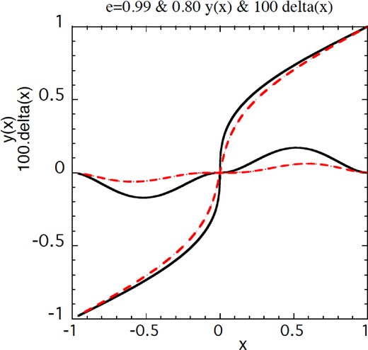
Figure 1.
The exact graphs satisfying Kepler's equation for e = 0.99 (top) and e = 0.8 (dashed just below) together with 100 times the error in x of the approximation (10) These errors never exceed 0.002 and will be reduced by a further factor of about 10 in the approximation (11).
In practice, choosing α so that x = x2, which is about 0.527 at e = 1, reduces the error δx by a factor which can be up to 16, so the final result as shown in Fig. 2 is good to better than 0.000 12!
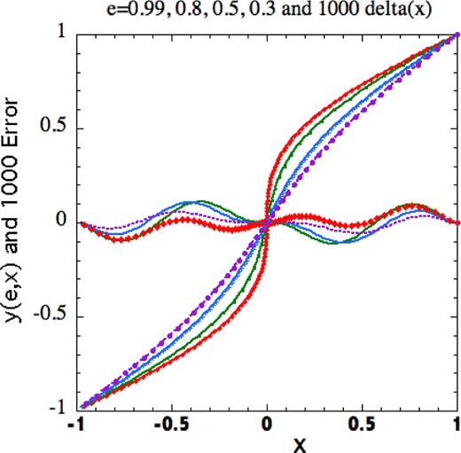
Figure 2.
Graphs of the exact relationships y(e, x) for e = 0.99(top), 0.8, 0.5 and 0.3 together with graphs of 1000 times the errors in x (at given y) of the approximate formula (11). These errors never exceed 0.000 12.
2.2 Solving the cubic
Multiplying up equation (11), the result takes the form
thus, the
fi are functions of
e and
x. By setting
|$\tilde{y}=y+f_2/(3f_3)$|, this equation can be put in the form
On making the substitution
|$\tilde{y}=w-p/w$| our equation, when multiplied by
w3, becomes quadratic in that variable:
w6 − 2
qw3 =
p3 so the solution is
Evidently
C− = −(
p3/
q2)(1/
C+) so returning to
y itself
which is clearly symmetrical between
C− and
C+ and gives our solution for
y(
x). The maximum errors in
y are somewhat less than the maximum errors in
x seen in Fig.
2. e.g. for
e = 0.99 and
e = 0.8 the |δ
y| are everywhere less than 0.000 06.
3 THE ANGLE AT THE CENTRE OF FORCE
The orbits are of the form (3) so
e*,
m and
k are known; thus from equation (3) and above,
|$\tilde{e}$| is known and
Tr is given in Lynden-Bell (
2015), so for any chosen time
t,
x is known. From the solution to the cubic above
|$y(\tilde{e},x)$| is known, so
|$\chi =\pi y(\tilde{e},x)$| is known. For general bound orbits, the angle χ is related to the angle ϕ at the centre of force (Kepler's true anomaly) by the relationships which are the same as Kepler's when expressed in terms of
e* (not
|$\tilde{e})$| but with
mϕ written for ϕ, vis
so with χ known,
mϕ and thus ϕ are easily found. For Kepler's case
|$m=1,\ \ e^*=\tilde{e}=e$|. Thus, we have found the angle at the force-centre as a function of the time since pericentric passage.
I thank the referee for his advice and references that together have led to a simpler and more accurate formulation.
REFERENCES
,
Solving Kepler's Equation Over Three Centuries
,
1993
Richmond, VA
Willmann-Bell Inc.
,
MNRAS
,
2008
, vol.
386
pg.
245
,
MNRAS
,
2010
, vol.
386
pg.
1937
,
Celest. Mech. Dyn. Astron.
,
1995
, vol.
63
pg.
101
,
Celest. Mech. Dyn. Astron.
,
1987
, vol.
40
pg.
329
,
AJ
,
2006
, vol.
131
pg.
1347
© 2014 The Author Published by Oxford University Press on behalf of the Royal Astronomical Society


