


Abstract
We investigate the mass–metallicity relation and its dependence on galaxy physical properties with a sample of 703 Lyman-break analogues (LBAs) in local Universe, which have similar properties to high-redshift star-forming galaxies. The sample is selected according to Hα luminosity, L(Hα) > 1041.8 erg s−1, and surface brightness, I(Hα) > 1040.5 erg s−1 kpc−2, criteria. The mass–metallicity relation of LBAs harmoniously agrees with that of star-forming galaxies at z ∼ 1.4–1.7 in stellar mass range of 108.5 M⊙ < M★ < 1011 M⊙. The relation between stellar mass, metallicity and star formation rate of our sample is roughly consistent with the local fundamental metallicity relation. We find that the mass–metallicity relation shows a strong correlation with the 4000 Å break; galaxies with higher 4000 Å break typically have higher metallicity at a fixed mass, by 0.06 dex in average. This trend is independent of the methodology of metallicity. We also use the metallicity estimated by Te-method to confirm it. The scatter in mass–metallicity relation can be reduced from 0.091 to 0.077 dex by a three-dimensional relation between stellar mass, metallicity and 4000 Å break. The reduction of scatter in mass–metallicity relation suggests that the galaxy stellar age plays an important role as the second parameter in the mass–metallicity relation of LBAs.
1 INTRODUCTION
Metallicity is a key parameter to probe the galaxy formation and evolution. Metal enrichment process of a galaxy involves many physical processes such as star formation, gas inflow and outflow. A correlation between metal abundance and galaxy total mass (gas and stellar mass) was found in the 1970s (Lequeux et al. 1979); typically, the greater mass galaxies have, the richer metallicity they are. Subsequently, Tremonti et al. (2004) confirmed the relation at z ∼ 0.1 by using ∼50 000 galaxies from the Sloan Digital Sky Survey (SDSS; Abazajian et al. 2004). They also showed that the mass–metallicity relation is tighter and more fundamental than the luminosity–metallicity relation. Recently, with deep survey of distant galaxies, many works investigate the mass–metallicity relation at intermediate (Maier et al. 2005; Savaglio et al. 2005; Zahid, Kewley & Bresolin 2011; Pérez-Montero et al. 2013) and high redshifts (Erb et al. 2006; Maiolino et al. 2008; Mannucci et al. 2009; Laskar, Berger & Chary 2011; Kulas et al. 2013; Yuan, Kewley & Richard 2013). The mass–metallicity relation at high redshift is shifted to lower metallicity compared to the local relation.
The scatter in the mass–metallicity relation is an important clue to understand the metal enrichment history of a galaxy. Many galaxy physical parameters are found to be correlated with the mass–metallicity relation, and likely to contribute to scatter in this relation. In the local Universe, the most widely investigated parameter is star formation rate (SFR; Ellison et al. 2008; Lara-López et al. 2010; Mannucci et al. 2010; Yates, Kauffmann & Guo 2012; Andrews & Martini 2013). Mannucci et al. (2010) found that galaxies with higher SFR typically have lower metallicities at a fixed mass. They proposed that the scatter in mass–metallicity relation could be significantly reduced by the relation between stellar mass, metallicity and SFR (fundamental metallicity relation, FMR). They argued that the local FMR does not evolve out to z ∼ 2.5. However, the FMR is found to be dependent on methodology (Yates et al. 2012; Andrews & Martini 2013) and aperture correction factor (Sánchez et al. 2013). In addition to SFR, many other works also suggest that the mass–metallicity relation is dependent on other physical parameters, such as optical colour (Tremonti et al. 2004), galaxy size (Ellison et al. 2008), morphology (Sol Alonso, Michel-Dansac & Lambas 2010) or gas mass fraction (Hughes et al. 2013). Studying the parameter dependence of mass–metallicity at high redshift is rather difficult because of limited size of the sample. Recently, Yabe et al. (2013) and Zahid et al. (2014a) severally obtained spectra of hundreds of star-forming galaxies (SFGs) at z ∼ 1.4–1.7 and analysed the parameter dependence of the mass–metallicity relation at this redshift range. However, with different sample sizes and parameter ranges, Zahid et al. (2014a) found evidence for the dependence on SFR, while no clear trend with SFR was found in the sample in Yabe et al. (2013).
To study the star formation properties of high-redshift SFGs in more detail, Heckman et al. (2005) and Hoopes et al. (2007) selected a local population of UV bright compact galaxies, named as supercompact UV luminous galaxies (UVLGs) or Lyman-break analogues (LBAs). The LBAs resemble Lyman-break galaxies (LBGs) in many aspects, including luminosity, stellar mass, SFR, extinction and metallicity (Basu-Zych et al. 2007; Hoopes et al. 2007; Buat et al. 2009; Overzier et al. 2011; Elmegreen et al. 2013). Hoopes et al. (2007) and Overzier et al. (2010) compared the mass–metallicity relation of UV selected LBAs with the relation of local SFGs (Tremonti et al. 2004) and UV selected LBGs at z ∼ 2.2 (Erb et al. 2006). They found that LBAs have similar metallicity to that of local SFGs at massive end (>1010.5 M⊙) and high-redshift LBGs at lower masses (<1010.5 M⊙). The high-redshift LBGs are less metal enriched than the local SFGs by a factor of 2 around (Erb et al. 2006). Here, with a larger sample, we compare the mass–metallicity relation with high-redshift SFGs in more detail and analyse the parameter dependence of the relation of LBAs. As a good representative of high-redshift SFGs in local Universe, a study of the correlation between the gas metallicity and other galaxy properties of LBAs could improve our knowledge about the metal enrichment process in LBAs and high-redshift SFGs.
Throughout this paper, we adopt the cosmological parameters with H0 = 70 km s−1 Mpc−1, ΩΛ = 0.73 and Ωm = 0.27.
2 SAMPLE SELECTION
2.1 Lyman-break analogues
Heckman et al. (2005) and Hoopes et al. (2007) selected a local compact SFG population (i.e. supercompact UVLGs) which is considered to be local analogues of LBGs. The selection criteria are based on far-ultraviolet (FUV) luminosity (L1530 > 2 × 10¹⁰ L⊙) and surface brightness (I1530 > 109 L⊙ kpc−2). Since FUV is sensitive to the dust attenuation, selection based on FUV may bias against dusty galaxies. Besides, Hα is also an excellent index of star formation and less sensitive to dust attenuation than FUV. Therefore, we obtain our sample by using Hα luminosity and surface brightness from SDSS Data Release 10 (DR10; Ahn et al. 2013). We use the emission-line fluxes, stellar masses and 4000 Å break, |$D_{\rm n}(4000)$|, derived by the MPA-JHU group (Brinchmann et al. 2004). A careful subtraction of stellar absorption-line spectrum is performed before measuring the emission lines (Kauffmann et al. 2003). As noted by Groves, Brinchmann & Walcher (2012), the equivalent width (EW) of Hβ in the MPA-JHU catalogue is underestimated by ∼ 0.35 Å. Since the minimum EW of Hβ of LBAs is 10.7 Å, this correction is negligible.
The selection criteria for LBAs are (1) redshift 0.05 < z < 0.30; (2) Hα luminosity L(Hα) > 1041.8 erg s−1; (3) Hα surface brightness I(Hα) > 1040.5 erg s−1 kpc−2; (4) |$D_{\rm n}(4000)$| is less than 1.1; (5) the log stellar mass error is less than 0.3 dex; (6) signal-to-noise (S/N) of (Hα) higher than 10. The lower redshift limit is set in order to ensure that the [O ii] λ3727 line is located in the spectral range of SDSS (3800–9200 Å). Hα surface brightness |$I({\rm H\alpha})=L({\rm H\alpha})/2\pi r_{50,i}^2$|, where r50, i is the half-light radius of objects in the SDSS i-band image. We use scalelength from the exponential model fit of the SDSS i-band image as the half-light radius at the Hα band. We do not correct Hα flux in our selection criteria for the intrinsic dust attenuation to be consistent with the uncorrected FUV criteria above. The thresholds of Hα luminosity and surface brightness are set to be comparable (i.e. with the same unobscured SFR) with FUV criteria of supercompact UVLGs. We set a |$D_{\rm n}(4000)$| upper limit to exclude intrinsic red (i.e. old) emission-line galaxies. Since no stellar mass error is available in the MPA-JHU catalogue, we defined the error as half of the difference between the 84th percentile and 16th percentile stellar mass probability distribution function (i.e. lgm_tot_p84 and lgm_tot_p16 index) in the MPA-JHU catalogue. About 7 per cent of galaxies have stellar mass error systematically higher than the major sample and the dividing point is at ∼0.3 dex. These galaxies also deviate the major sample in the mass–metallicity diagram, which may be due to the poorly determined stellar mass. The Hα S/N criterion removes another six galaxies which do not have reliable detection of the Hα line. In total, 817 galaxies in the SDSS DR10 are selected by our Hα criteria.
Since fibre spectra only measure the centre regions of extended objects, aperture corrections are needed to get integrated properties. One simple estimate of aperture correction factor is the difference between fibre and total magnitude (Hopkins et al. 2003). Owing to lack of knowledge about the spatial distribution of emission line, the correction factors for emission line are always estimated by the use of adjacent broad-band photometry. We use SDSS i-band photometry to roughly estimate the aperture correction factors. The median correction factor of LBAs is only 1.5 (0.18 dex), which indicates that two thirds of light is included in the SDSS 3 arcsec fibre. The aperture correction factor is rather small compared to normal SFGs because LBAs are compact objects with typical sizes of 1 ∼ 2 kpc (Overzier et al. 2009, 2010). A comparison between the fibre SFR and the aperture-corrected SFR measurement in the MPA-JHU galSpecExtra catalogue1 (i.e. sft_tot_p50 index) indicates smaller correction factors with a median of 1.2 (0.07 dex). The aperture-corrected SFR in the MPA-JHU catalogue is derived from combining emission line within the fibre and aperture corrections by fitting model (Gallazzi et al. 2005; Salim et al. 2007) into the photometry outside the fibre. With such high fibre covering fraction, the metallicity and dust extinction calculated with fibre spectra could represent the global values (Kewley, Jansen & Geller 2005). The aperture correction method always depends on the assumption that the distributions of emission line (ionized gas emission) and broad-band photometry (stellar emission) are identical outside the fibre, which may introduce systematic errors in aperture correction. These systematic errors could introduce many extended normal SFGs which have more extended continuum emission than emission lines. Besides, the aperture correction factor for LBAs is rather small and the majority of them could be selected by criteria within fibre. Therefore, we do not correct the aperture effect for Hα flux in sample selection. However, we will use aperture-corrected SFR and gas mass fraction in subsequent analysis.
The AGN contamination is excluded from our sample by the BPT diagram (Baldwin, Phillips & Terlevich 1981). Fig. 1 shows the distribution of LBAs in the |$\rm {log}([N\,{\scriptscriptstyle II}]/{\rm H\alpha})$| versus |$\rm {log}([O\,{\scriptscriptstyle III}]/{\rm H\beta})$| diagram. We cross-match the 817 galaxies with GALEX all sky survey catalogue (Martin et al. 2005) and divide it into two subsamples. Galaxies that satisfy the FUV criteria of supercompact UVLGs are grouped into the ‘UV’ selected subsample and others into the ‘non-UV’ selected subsample. The red asterisks and blue circles represent the ‘non-UV’ and ‘UV’ selected subsamples, respectively. It can be seen from Fig. 1 that the ‘non-UV’ and ‘UV’ LBAs show similar distribution of line ratios which suggests that they have similar ionization properties. A two-sample Kolmogorov–Smirnov test suggests that, in |$\rm {log}([N\,{\scriptscriptstyle II}]/{\rm H\alpha})$| and |$\rm {log}([O\,{\scriptscriptstyle III}]/{\rm H\beta})$| distributions, the differences between two subsamples are significant at a level less than 2σ. The solid and dotted lines are the demarcation curves between SFGs and AGNs derived by Kauffmann et al. (2003) and Kewley et al. (2001), respectively. Galaxies located between these two lines are often classified as composite objects which may host a mixture of AGN and star formation. We adopt the criteria of Kauffmann et al. (2003) to remove AGNs. The AGN fractions in the ‘UV’ and ‘non-UV’ subsample are 14 and 12 per cent, respectively. Finally, 703 galaxies ( 524 ‘non-UV’ and 179 ‘UV’) remain and constitute our LBA sample, with a median redshift of 0.20 ± 0.04.

2.2 SFGs in SDSS
To compare the parameter dependence of the mass–metallicity relation between LBAs and local normal SFGs, we select an SFG sample from SDSS DR10 according to the selection criteria in Mannucci et al. (2010). The major selection criteria are (1) redshift between 0.07 and 0.3; (2) S/N (Hα) >25; (3) dust attenuation Av < 2.5. Finally, 152 477 galaxies remain in the normal SFG sample. Fig. 2 shows the distributions of LBAs and SFGs in the dust extinction-corrected Hα luminosity versus Hα surface brightness diagram. It can be seen that LBAs are extreme cases of normal SFGs with high SFR and SFR surface densities.
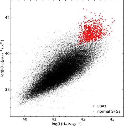
Hα surface bright versus Hα luminosity. Hα luminosity is corrected for dust extinction. Stars are normal SFGs and red circles are LBAs.
3 MASS–METALLICITY RELATION
There are several methods to determine the metallicity of an emission-line galaxy. The ‘Te-method’, which is regarded as a direct way to obtain metallicity, is based on the fact that metallicity is anticorrelated with the electron temperature Te. The electron temperature can be obtained using the ratio of the auroral to nebular emission lines of the same ion. Since the auroral lines are always very weak, many empirical and theoretical methods are developed (classified according to Kewley & Ellison 2008). The empirical calibrations such as ‘N2 method’ ([N ii]/Hα; Pettini & Pagel 2004), ‘O3N2 method’ (([O iii]/Hβ)/([N ii]/Hα); Pettini & Pagel 2004) and ‘R23 method’ (([O ii] λ3727+[O iii] λλ4959, 5007)/Hβ; Pilyugin & Thuan 2005) are calibrated by the relation between strong line ratios and the Te-derived metallicities. The theoretical methods are also based on strong line ratios but calibrated by theoretical photoionization models. Although these methods are all based on strong line ratios, the metallicity derived from different methods can vary up to 0.7 dex (Shi et al. 2005; Kewley & Ellison 2008). The origin of the discrepancy between different metallicity calibrations is not clear yet.
Obtaining spectra with wide wavelength range is difficult and time-consuming for high-redshift galaxies. Therefore, the empirical N2 method, based on two adjacent lines (i.e. |$[\rm N\,{\scriptscriptstyle II}]\,\lambda 6584$| and Hα), is widely used in high-redshift works to obtain metallicity. Another advantage of the N2 method is that it is insensitive to dust attenuation, because of the adjacency of |$[\rm N\,{\scriptscriptstyle II}]\,\lambda 6584$| and Hα. The drawback of the N2 method is the saturation of N2 index above approximate solar abundance and dependence on ionization parameters. With the significant discrepancies between different metallicity calibrations, comparison with other works should be very careful. It is more straightforward to use the same metallicity calibration. Since one main goal of this paper is to compare the mass–metallicity relations of LBAs and high-redshift SFGs, the empirical N2 method (Pettini & Pagel 2004) is used to determine metallicities for our LBA sample.
The left-hand panel of Fig. 3 shows the distribution of LBAs in the mass–metallicity diagram. Galaxies in the UV subsample are represented as blue circles and those in the non-UV subsample as red asterisks. It can be seen that these two subsamples have a similar distribution in terms of mass and metallicity. A two-sample Kolmogorov–Smirnov test suggests that, in mass and metallicity distributions, differences are significant at a less than 2σ level. The agreement between the UV and non-UV subsample suggests that the deviation of mass–metallicity relation between UV selected LBAs and local SFGs, which was reported by Hoopes et al. (2007), could not be explained by selection bias against dusty objects. The deviation may be due to the high SFR and |$D_{\rm n}(4000)$| of LBAs compared to normal SFGs, which will be discussed in Section 4.
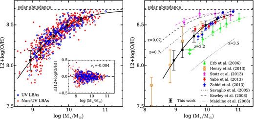
Left-hand panel: the mass–metallicity diagram for galaxies in UV subsample (blue circles) and non-UV subsample (red asterisks). The solid black curve is the best-fitting line and the black squares are binned data. Error bars are the median absolute deviation from median in each bin. The bottom-right inset panel is the metallicity residuals from the logarithmic fit. Right-hand panel: comparison of mass–metallicity relation of LBAs with the relations at high redshifts. The horizontal dashed line is solar metallicity (12+log(O/H) = 8.69; Asplund et al. 2009).
The mass–metallicity relation at high redshift has been largely exploited in recent years (z = 0.84 and 1.47, Stott et al. 2013; z ∼ 1.4, Yabe et al. 2013; z ∼ 1.6, Zahid et al. 2014a,b; z ∼ 1.76, Henry et al. 2013; z ∼ 2, Erb et al. 2006 and Hayashi et al. 2009; z ∼ 3.5, Maiolino et al. 2008). The comparison of the mass–metallicity relation between LBAs and these high-redshift SFG samples is presented in the right-hand panel of Fig. 3. The local SFG sample (z ∼ 0.07; Kewley & Ellison 2008) is also included as reference. For a fair comparison, the masses are corrected to Kroupa initial mass function (Kroupa 2001) based stellar masses and metallicities to the empirical N2 method (Pettini & Pagel 2004) through the conversion in Maiolino et al. (2008).
It is worth noticing that the mass–metallicity relation of LBAs is in remarkable consistency with that at z ∼ 1.4–1.7 (Yabe et al. 2013; Zahid et al. 2014a). The consistency is extended to lower masses by Henry et al. (2013), who investigated the mass–metallicity relation of low-mass galaxies at z ∼ 1.76 at mass down to ∼108.5 M⊙. Stott et al. (2013) measured the mass–metallicity relation for a combined sample of galaxies at z = 0.84 and 1.47. However, they found that the mass–metallicity relation at z = 0.84 and 1.47 is comparable to the local mass–metallicity relation and concluded that there is no evolution of the mass–metallicity relation with redshift. They argued that the origin of evolution in the mass–metallicity relation is selection bias in galaxies with bright UV luminosity and high SFR which tend to be more metal poor than normal galaxies. However, Zahid et al. (2014a) selected an SFG sample at z ∼ 1.6 based on sBzK selection (Daddi et al. 2004), which does not suffer the selection bias mentioned in Stott et al. (2013), and argued that the evolution of mass–metallicity relation seems to be real.
It can be seen in Fig. 3 that massive LBAs have metallicities similar to that of normal SFGs at z ∼ 0.07. However, at lower masses, the metallicity discrepancy between LBAs and local SFGs becomes larger, which is consistent with the deviation found in Hoopes et al. (2007). Savaglio et al. (2005) measured the mass–metallicity relation of SFGs at z ∼ 0.7 (dot–dashed line in the right-hand panel of Fig. 3) and interpreted the flattening of mass–metallicity relation from z ∼ 0.7 to z ∼ 0.1 as a result of downsizing evolution of galaxy population. Massive galaxies at high redshift reach high metallicity, while low-mass systems enrich their interstellar medium on long time-scales and are still converting gas into stars at present time. In terms of downsizing scenario, the local LBAs are less evolved compared to the local SFGs. It is also interesting to note that the mass–metallicity relation at z ∼ 1.4–1.7 (Yabe et al. 2013; Zahid et al. 2014a), supplemented by the low-mass galaxies from Henry et al. (2013), is roughly parallel to that at z ∼ 2.2 (Erb et al. 2006) and z ∼ 3.5 (Maiolino et al. 2008). The shape of mass–metallicity relation does not significantly change from z ∼ 3.5 to z ∼ 1.4–1.7, which suggests a mass-independent metal enrichment process. This is quite different from the downsizing/mass-dependent evolution at lower redshift. However, a detailed consideration of sample selection biases at each epoch and larger sample at high redshift with sufficient low-mass galaxies is required to confirm or reject this trend.
4 DEPENDENCE OF THE MASS–METALLICITY RELATION ON GALAXY PROPERTIES
The dependence of the mass–metallicity relation on galaxy properties has been explored by many works (Ellison et al. 2008, Mannucci et al. 2010, Lara-López et al. 2010, Yates et al. 2012, Sánchez et al. 2013 and Andrews & Martini 2013 for local SFGs; Stott et al. 2013, Yabe et al. 2013 and Zahid et al. 2014a for high-redshift SFGs). Here, we examine that for LBAs and compare with the parameter dependence of the mass–metallicity relation at high redshift. The parameters examined are the intrinsic SFR, |$D_{\rm n}(4000)$|, E(B − V) and gas mass fraction. The intrinsic SFR is derived from Hα luminosity by use of the relation from Kennicutt (1998). We correct Hα luminosity for dust extinction by using the Balmer decrement method and adopting the Calzetti extinction law (Calzetti et al. 2000). We also account for the aperture effect using the correction method mentioned in Section 2.1. The obtained SFR ranges from 4 to 100 M⊙ yr−1 with a median of 15.9 ± 5.7 M⊙ yr−1. The corrected SFR is consistent with the aperture-corrected SFR measurement in the MPA-JHU catalogue. The E(B − V), which is derived from the Balmer decrement method with Calzetti extinction law, ranges from 0.0 to 0.49 mag with a median of 0.17 ± 0.06. The |$D_{\rm n}(4000)$| is taken from the ‘d4000_n’ index in the MPA-JHU galSpecIndx catalogue2 (Brinchmann et al. 2004) and calculated according to the Balogh et al. (1998) definition. The LBA sample has |$D_{\rm n}(4000)$| value ranging from 0.45 to 1.1. To accurately estimate the gas mass, CO measurements, which is extremely time-consuming for a large sample of normal SFGs, are necessary. Alternatively, a correlation between surface densities of gas mass and star formation was found and independent of galaxy type (i.e. the Schmidt law; Kennicutt 1998). Assuming such a law is suitable for LBAs, we could roughly estimate the gas mass from dust and aperture-corrected Hα luminosity and size of galaxies. This indirect method is also used by Tremonti et al. (2004) and Erb et al. (2006) to derive gas mass fractions. The size of galaxy, which represents the size of the emission region of stellar component, is assumed to be the same to that of Hα emission region. The obtained gas mass fraction, Mgas/(Mgas + M★), ranges from 0.01 to 0.79 with a median of 0.35 ± 0.14.
To explore the effect of different metallicity calibration methods on the parameter dependence of the mass–metallicity relation, we also use the method given in Mannucci et al. (2010) to determine the metallicities of LBAs and normal SFGs. Two independent calibrations based on the N2 to R23 ratio as described in Maiolino et al. (2008) are used (hereafter N2+R23 calibration). When both two calibrations are available (i.e. log(|$[\rm N\,{\scriptscriptstyle II}]/{\rm H\alpha}$|) < −0.35 and log(R23) < 0.9) and the difference between the two derived metallicities is less than 0.25 dex, the average of the two values is the final metallicity. It is suggested that the R23 calibration has double-valued solutions. Since the |$[\rm N\,{\scriptscriptstyle II}]/[O\,{\scriptscriptstyle II}]$| ratio is a strong function of metallicity (Kewley & Dopita 2002), we use the |$[\rm N\,{\scriptscriptstyle II}]/[O\,{\scriptscriptstyle II}]$| ratio to break the R23 degeneracy. We take the higher metallicity value for galaxies with log(|$[\rm N\,{\scriptscriptstyle II}]/[O\,{\scriptscriptstyle II}]$|) >− 1.2 and lower value for galaxies with log(|$[\rm N\,{\scriptscriptstyle II}]/[O\,{\scriptscriptstyle II}]$|) <−1.2.
The LBA sample is divided into 12 mass bins with bin size of 0.2 dex. To study the parameter dependence of the mass–metallicity relation, we divide the objects in each mass bin into two groups according to the median value of the parameter in the mass bin. Metallicity in Figs 4 and 5 is calculated using empirical N2 method and N2+R23 calibrations, respectively. The circles and triangles in Figs. 4 and 5 represent the median of mass and metallicity for the group with high and low value, respectively. The median absolute deviation from median value is used to estimate the spread of x- and y-axes and represented as error bar in Figs 4 and 5. Three bins in Figs 4 and 5, which have objects less than 20, are excluded for analysis. The median value of each parameter in each stellar mass bin is listed in Table 1.

The dependence of the mass–metallicity relation on the galaxy physical parameters, including SFR, |$D_{\rm n}(4000)$|, E(B − V) and gas mass fraction. In each mass bin, we divide galaxies into two groups by the parameter. We calculate the median of mass and metallicity for each group in each bin. The median absolute deviation from median value is used to estimate the spread and represented as error bar. The deviation shown in the head of each panel represents the average offset in each bin.

Parameter dependence of the mass–metallicity relation. For each parameter and stellar mass bin, the median values are listed.
| ID | log(M★/M⊙) | 12+log(O/H) [N2] ([N2+R23]) | SFR (M⊙ yr−1) | |$D_{\rm n}(4000)$| | E(B − V) | Gas fraction | Na |
|---|---|---|---|---|---|---|---|
| 1 | 8.96 ± 0.03 | 8.06 ± 0.12 (8.15 ± 0.14) | 8.3 ± 2.2 | 0.69 ± 0.04 | 0.08 ± 0.04 | 0.61 ± 0.05 | 25 (24) |
| 2 | 9.12 ± 0.05 | 8.14 ± 0.07 (8.23 ± 0.10) | 9.7 ± 2.4 | 0.77 ± 0.07 | 0.08 ± 0.05 | 0.55 ± 0.06 | 68 (61) |
| 3 | 9.28 ± 0.05 | 8.24 ± 0.07 (8.39 ± 0.10) | 13.2 ± 3.4 | 0.85 ± 0.06 | 0.11 ± 0.04 | 0.52 ± 0.07 | 98 (90) |
| 4 | 9.48 ± 0.04 | 8.31 ± 0.06 (8.47 ± 0.08) | 15.0 ± 5.4 | 0.91 ± 0.06 | 0.13 ± 0.04 | 0.46 ± 0.08 | 92 (86) |
| 5 | 9.70 ± 0.04 | 8.40 ± 0.05 (8.60 ± 0.07) | 15.6 ± 4.2 | 0.98 ± 0.04 | 0.17 ± 0.04 | 0.36 ± 0.06 | 99 (97) |
| 6 | 9.90 ± 0.05 | 8.47 ± 0.04 (8.69 ± 0.06) | 16.5 ± 4.9 | 1.02 ± 0.03 | 0.20 ± 0.05 | 0.29 ± 0.07 | 117 (115) |
| 7 | 10.09 ± 0.06 | 8.53 ± 0.05 (8.77 ± 0.08) | 19.3 ± 5.1 | 1.05 ± 0.03 | 0.23 ± 0.05 | 0.22 ± 0.05 | 82 (80) |
| 8 | 10.28 ± 0.05 | 8.55 ± 0.04 (8.80 ± 0.05) | 27.9 ± 9.7 | 1.05 ± 0.03 | 0.27 ± 0.04 | 0.20 ± 0.05 | 59 (59) |
| 9 | 10.48 ± 0.05 | 8.59 ± 0.02 (8.85 ± 0.05) | 34.0 ± 7.8 | 1.07 ± 0.02 | 0.30 ± 0.05 | 0.16 ± 0.03 | 34 (33) |
Note.aNumber of galaxies in each stellar mass bin. The value in parentheses is presented for LBAs which have metallicity determined by using the N2+R23 calibration method.
4.1 SFR
There is no systematical offset between high-SFR and low-SFR group galaxies in Fig. 4. However, systematic deviation seems to exist in intermediate-mass bins in Fig. 5. The relation between mass, metallicity and SFR in local SFGs has been discovered and studied in many recent works (Ellison et al. 2008; Lara-López et al. 2010; Mannucci et al. 2010; Yates et al. 2012; Andrews & Martini 2013; Sánchez et al. 2013; Stott et al. 2013). Galaxies with higher SFR tend to have lower metallicities at a fixed stellar mass (Ellison et al. 2008; Mannucci et al. 2010; Andrews & Martini 2013). Although FMR is found in local Universe, the relation between stellar mass, metallicity and SFR in high-redshift galaxies is not very clear yet. The mass–metallicity relation is dependent on SFR in the sample of Zahid et al. (2014a) at z ∼ 1.6. However, Yabe et al. (2013) did not find systematical trend that galaxies with higher SFR have lower metallicity in their SFG sample at z ∼ 1.4.
Based on the local relation between stellar mass, metallicity and SFR, Mannucci et al. (2010) proposed that the scatter in the mass–metallicity relation could be significantly reduced by including SFR as another free parameter. The three-dimensional relation is named as the ‘fundamental metallicity relation’ (FMR). They defined a new quantity μα, which is a combination of stellar mass and SFR (μα = log(M★/ M⊙) − αlog(SFR)). They found that α = 0.32 minimizes the scatter in the local FMR and the value does not change in the FMR of SFGs at z < 2.5. To verify whether our LBA sample is consistent with the FMR, we plot the FMR for LBAs in Fig. 6. The solid curve is the FMR in Mannucci et al. (2010), which is not corrected for the aperture effect. We also calculated the FMR of normal SFGs, shown as dashed curve, using aperture-corrected SFR from the MPA-JHU catalogue. It can be seen that the FMR of normal SFGs with aperture-corrected SFR shifts left to the original FMR in Mannucci et al. (2010) with fibre SFR, which is consistent with the estimate of FMR shift in Zahid et al. (2014a). The FMR of LBAs is roughly consistent with both two FMRs of local normal SFGs. We note that there is better agreement between local FMR and the relation of LBAs if we use SFRs without aperture corrections. However, the FMR connects global properties of a galaxy and SDSS fibre. SFR is not an appropriate measurement to derive such a relation. Since the mass–metallicity relation of LBAs is not strongly dependent on SFR, an FMR that combines stellar mass and SFR does not reduce the scatter in the mass–metallicity relation notably. It should be noted that LBAs are subsample of normal SFGs with high SFR. The slight SFR dependence may be due to the relative narrow SFR range of LBA sample.
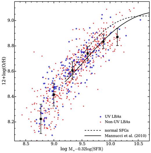
The FMR of our LBA sample. The metallicity is calculated by the same calibration in Mannucci et al. (2010). The binned data points and error bars are calculated by the same procedure as mentioned in Fig. 4. The solid line is the metallicity–μ0.32 relation for the local SFG sample by Mannucci et al. (2010). The dashed curve is the FMR of normal SFGs using aperture-corrected SFR.
4.2 |$D_{\rm n}(4000)$|
Yabe et al. (2013) found that the metallicity of galaxies at high redshift correlates with the rest-frame NUV (near-ultraviolet-optical)–optical colour at a fixed mass. Galaxies with redder colour tend to have higher metallicities. Hayashi et al. (2009) suggested that the difference in observed R − K colour, which covers the 4000 Å break, may contribute to the discrepancy between the mass–metallicity relation they derived at z ∼ 2 and that from Erb et al. (2006). It can be seen from the upper-right panel of Fig. 4 that there is strong correlation between the mass–metallicity relation and |$D_{\rm n}(4000)$| for our LBA sample. The trend could also be seen from Fig. 5 which suggests that the correlation with |$D_{\rm n}(4000)$| is not dependent on the metallicity methodology. It is worth noting that the average offset between high- and low-|$D_{\rm n}(4000)$| groups is as large as 0.06 dex, which is the largest deviation among the four galaxy physical parameters. Since the metallicity calibrations based on strong line ratio have large uncertainties, we also use the Te-method to compare the metallicity of high- and low-|$D_{\rm n}(4000)$| groups. We split our sample into nine stellar mass bins from 109 to 1011 M⊙. Each size is 0.2 dex. Each stellar mass bin is then divided into two groups according to the median value of |$D_{\rm n}(4000)$|. Then, we follow the spectra stack and continuum subtraction steps of Andrews & Martini (2013). Fig. 7 shows the reduced rest-frame spectra of 4250–4450 Å of each group in each mass bin. The spectra have been normalized to dust-corrected Hβ flux. The high-|$D_{\rm n}(4000)$| groups are shown in upper row. In each mass bin, it can be seen that the [O iii] λ4363 auroral line is much stronger in the low-|$D_{\rm n}(4000)$| groups. It is suggested that the strength of [O iii] λ4363 line is strongly correlated with the electron temperature and anti-correlated with metallicity. Therefore, metallicity based on the Te-method should be higher in high-|$D_{\rm n}(4000)$| groups. Since the [O iii] λ4363 line is too weak in most mass bins to be reliably measured, we calculate the metallicity of the first two mass bins using the Te-method reported by Izotov et al. (2006). The results are shown as title in the corresponding panel. The metallicity difference in the first two mass bins between high-|$D_{\rm n}(4000)$| and low-|$D_{\rm n}(4000)$| groups is ∼ 0.15 dex, which is comparable to the value in Figs 4 and 5.
![Comparison of stacked spectra between high- and low-$D_{\rm n}(4000)$ groups. From left to right, the nine columns are stacked spectra of the nine stellar mass bins from 109 to 1011 M⊙. High- and low-$D_{\rm n}(4000)$ groups are displayed at upper and lower rows. The dashed line in each row marks the [O iii] λ 4363 line. The title of the first two columns shows the metallicities calculated by using the Te-method.](https://oup.silverchair-cdn.com/oup/backfile/Content_public/Journal/mnras/446/2/10.1093_mnras_stu2184/2/m_stu2184fig7.jpeg?Expires=1750485072&Signature=wnXoGCcd9ZmDKhnXK7q4sncEbHjQYg8FjPj~4xudX3rDUy8BdbSjvQHdVy1uV3FeRx~3sAcWmVSg3Dn-CMeqSP0dPtLBbPKMTsxhuNlZce1~uYkmzQYTuVCC34rZNmL-XWJ08msOGWSvSj2NhvePoo1OPNwRgPg4xwHUeqNFna~XTJtjyipH99AbFWUHhkhG4Y6SkRAxrKbwd5WyyCvqJ7BMNPPJ7b5o2Lg7vNgtNNk8xVnnJLpJ2eISkMnHpA6aes7y-ZMJDSnWkXt0LcKvXkaZC5bZFDYjzjr-y4ijxW9KdtpGY80NEUo7ZKlPHBy5WinQurIPEmzg4Cl0xYU8Vg__&Key-Pair-Id=APKAIE5G5CRDK6RD3PGA)
Comparison of stacked spectra between high- and low-|$D_{\rm n}(4000)$| groups. From left to right, the nine columns are stacked spectra of the nine stellar mass bins from 109 to 1011 M⊙. High- and low-|$D_{\rm n}(4000)$| groups are displayed at upper and lower rows. The dashed line in each row marks the [O iii] λ 4363 line. The title of the first two columns shows the metallicities calculated by using the Te-method.
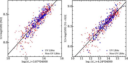
Metallicity as a function of ϕα. Left-hand panel is for the empirical N2 method and right-hand panel for the method combining N2 and R23 calibrations. Solid lines are best-fitting metallicity–ϕα relations. The dashed curve in the right-hand panel is the metallicity–ϕα relation of normal SFGs.
Since |$D_{\rm n}(4000)$| is considered as a good indicator of galaxy stellar age (Kauffmann et al. 2003), the dependence on |$D_{\rm n}(4000)$| could be interpreted as: galaxies with elder stellar age always have higher metallicity at a fixed stellar mass. This trend seems to be understandable. Galaxies with the same current stellar mass did not produce the same amount of stellar mass along with their formation history. Actually, more stars in elder galaxies have left the stellar main sequence than those in younger galaxies with the same current stellar mass, in average. Therefore, the integral of stellar mass along with the lifetime of a galaxy should be higher for elder galaxies. Thus, elder galaxies experience more metal enrichment process (such as supernova and/or massive stellar wind) and have relative higher metallicities. Given this interpretation, the dependence on stellar age of the mass–metallicity relation is a natural result of passive evolution since one can only measure the current galaxy mass.
4.3 E(B − V)
There is a slight trend in the bottom-left panel of Fig. 4 that galaxies with higher E(B − V) tend to have higher metallicities. This trend seems to be weaker in Fig. 5 with metallicity determined using the N2+R23 method. The average offset in each mass bin between large and small E(B − V) is ∼ 0.03 dex. Similar trends are observed in a high-redshift galaxy sample at z ∼ 1.4–1.7 (Yabe et al. 2013; Zahid et al. 2014a). This trend could be comprehensible because E(B − V) reflects the dust extinction, while the dust content in a galaxy is strongly correlated with metal abundance in the galaxy (Heckman et al. 1998; Reddy et al. 2010). The average dependence on E(B − V), which is Δ[12 + log(O/H)]/ΔE(B − V) = 0.37 dex mag−1, is comparable with the E(B − V) dependence of galaxies at z ∼ 1.4 (0.56 dex mag−1) from Yabe et al. (2013).
4.4 Gas fraction
It can be seen in bottom right of Fig. 4 that the deviation between two group galaxies is slight and they are almost on the same mass–metallicity relation which resembles the behaviour of galaxy sample at z ∼ 1.4 (Yabe et al. 2013). It is noted by Yabe et al. (2013) that the dependence on gas mass fraction seems due to the mass–metallicity relation itself since the gas mass fraction correlates strongly with the stellar mass. It is worth noting that the dependence on gas mass fraction of mass–metallicity relation may be reflected by the dependence on SFR, since the estimation of gas mass is closely connected to the SFR. Hughes et al. (2013) found that the mass–metallicity relation is dependent on |$H\,{\scriptscriptstyle I}$| gas mass fraction; galaxies with higher gas fractions have lower oxygen abundances at a fixed mass. With limited data set of CO maps and large uncertainties in CO-to-H2 conversion factor, the dependence on H2 gas mass fraction is not clear yet.
5 SUMMARY
The main goal of this work is to study the mass–metallicity relation of LBAs and the dependence of this relation on galaxy properties. Since Hα suffers less dust attenuation than UV photons, we select LBA sample according to Hα luminosity and surface brightness criteria to obtain a larger LBA sample with less bias. In total, 703 galaxies are selected from the SDSS DR10 as our LBA sample, and only ∼ 25 per cent of them can be recognized by the previous FUV selection criteria. The main results and conclusion of this paper are as follows.
The mass–metallicity relation of LBAs is in good agreement with that of SFGs at z ∼ 1.4–1.7 in stellar mass range of 108.5 M⊙ < M★ < 1011 M⊙.
The mass–metallicity relation is found to be strongly correlated with |$D_{\rm n}(4000)$|; galaxies with higher |$D_{\rm n}(4000)$| typically have higher metallicity at a fixed mass. This trend is independent of the methodology of metallicity. We confirm the dependence on |$D_{\rm n}(4000)$| by using the Te-method for estimating metallicity of stacked spectra. A correlation of mass–metallicity relation with NUV–optical colour was found in Yabe et al. (2013) and is probably due to the correlation with |$D_{\rm n}(4000)$|. About 17 per cent of the total scatter in the mass–metallicity relation is due to the systematic effect with |$D_{\rm n}(4000)$|. This suggests that the galaxy stellar age plays an important role as a second parameter in the mass–metallicity relation of LBAs and even high-redshift SFGs.
The mass–metallicity relation of local normal SFGs is also found to be correlated with |$D_{\rm n}(4000)$|. There is good agreement between the three-dimensional relation of mass, metallicity and |$D_{\rm n}(4000)$| of normal SFGs and LBAs, which suggests a universal relation of different type of SFGs.
There is no strong correlation between the mass–metallicity relation of LBAs and SFR. The relation between stellar mass, metallicity and SFR of LBAs is roughly consistent with the local FMR. The lack of dependence on SFR may be due to the narrow range of SFR of LBA sample.
At a fixed mass, dustier galaxies typically have higher metallicities. This trend is consistent with SFGs at high redshift (Yabe et al. 2013; Zahid et al. 2014a).
The similarity of mass–metallicity relation and its dependence on galaxy properties between LBAs and high-redshift SFGs makes it more explicit that local LBAs are located at a similar evolution stage to SFGs at z ∼ 1.4–1.7.
We are grateful to referee and Roderik A. Overzier for all insightful suggestions and comments, and the MPA-JHU teams for their public measured quantities on SDSS galaxies. This work is supported by the National Natural Science Foundation of China (NSFC, Nos. 11225315, 1320101002, 11433005, and 11421303), the Strategic Priority Research Program ‘The Emergence of Cosmological Structures’ of the Chinese Academy of Sciences (No. XDB09000000), the Specialized Research Fund for the Doctoral Program of Higher Education (SRFDP, No. 20123402110037), and the Chinese National 973 Fundamental Science Programs (973 program) (2015CB857004).
J. H. Lian and J. R. Li contributed equally to this work.
