


Abstract
We announce a new facility in the spectral code cloudy that enables tracking the evolution of a cooling parcel of gas with time. For gas cooling from temperatures relevant to galaxy clusters, earlier calculations estimated the [Fe xiv] λ5303/[Fe x] λ6375 luminosity ratio, a critical diagnostic of a cooling plasma, to slightly less than unity. By contrast, our calculations predict a ratio of ∼3. We revisit recent optical coronal line observations along the X-ray cool arc around NGC 4696 by Canning et al., which detected [Fe x] λ6375, but not [Fe xiv] λ5303. We show that these observations are not consistent with predictions of cooling flow models. Differential extinction could in principle account for the observations, but it requires extinction levels (AV > 3.625) incompatible with previous observations. The non-detection of [Fe xiv] implies a temperature ceiling of 2.1 million K. Assuming cylindrical geometry and transonic turbulent pressure support, we estimate the gas mass at ∼1 million M⊙. The coronal gas is cooling isochorically. We propose that the coronal gas has not condensed out of the intracluster medium, but instead is the conductive or mixing interface between the X-ray plume and the optical filaments. We present a number of emission lines that may be pursued to test this hypothesis and constrain the amount of intermediate-temperature gas in the system.
1 INTRODUCTION
The X-ray-emitting hot intracluster medium (ICM) at the centres of cool core clusters of galaxies can have cooling times shorter than a Hubble time (see e.g. Fabian 2012). Heating, most likely from active galactic nuclei (AGN) feedback, prevents catastrophic cooling. However, the brightest cluster galaxies in these systems are observed to have substantial quantities of cool and cold gas and star formation relative to their non-cool core analogues, and it is widely believed that some residual cooling must occur.
If gas is cooling radiatively, then observations of intermediate-temperature gas could probe the cooling rates in these systems. Sanders et al. (2008) reported a temperature floor of ∼4 million K in their dispersive X-ray spectra of the Centaurus cluster. The detection of O vii at much lower levels than predicted by cooling flow models (Sanders & Fabian 2011) indicates that a dearth of 1–3 million K gas is common among cool clusters. If cooling at cluster centres is not impeded by heating mechanisms, it may proceed non-radiatively, e.g. through mixing.
Recently, Canning et al. (2011a, hereafter C11a) reported a detection of [Fe x] coronal line emission in NGC 4696, the brightest cluster galaxy in the nearby (z = 0.0104, 44.3 Mpc) Centaurus cluster. This line is sensitive to ∼million K gas. If the emission arises from cooling gas, their detection implies a high mass deposition rate of ∼20 M⊙ yr−1. However, they do not detect the higher excitation line of [Fe xiv].
This paper builds upon advances in the spectral simulation code cloudy, which permit simulations where the ionization is not in equilibrium with the local gas kinetic temperature (Chatzikos et al., in preparation). Lykins et al. (2013) describe the improvements in the atomic physics which underlies such simulations.
The outline of the paper is as follows. In Section 2, we present a brief overview of our numerical implementation of non-equilibrium cooling. In Section 3, we present modern calculations of the cooling efficiencies for the emission lines pursued by C11a and emphasize the improvements since Graney & Sarazin (1990, hereafter GS90). In Section 4, we establish that [Fe x] is optically thin. In Section 5, we update the mass deposition rate through [Fe x] and compare it to the mass deposition rate through the X-rays of Sanders et al. (2008). In Section 6, we use our cloudy simulations to rule out the possibility that the coronal line gas is a cooling condensation of the ambient ICM. Then, in Section 7 we use the non-detection of [Fe xiv] to constrain the temperature structure of the coronal gas, and in Section 8 we obtain its basic properties based on the detected [Fe x]. We discuss our results in Section 9 and summarize in Section 10.
2 SPECTRAL SIMULATIONS
This section outlines how we compute the spectrum of a cooling non-equilibrium parcel of gas. The calculations presented here were performed with version r9230 on the ‘dyna’ development branch of the spectral synthesis code cloudy (Ferland et al. 2013).
In all cases, we begin with a hot gas in collisional ionization equilibrium (CIE) at a preset temperature. We then allow the gas to freely cool, solving for the gas kinetic temperature, the non-equilibrium distribution of ionization (NEI), the gas cooling, and its spectrum.
The implementation of time-dependent physics within cloudy is discussed in detail in a separate paper (Chatzikos et al., in preparation). Briefly, our approach builds upon the infrastructure developed by Henney et al. (2005) to treat the structure of steady-state ionization fronts. In its normal mode of usage, cloudy uses a hierarchy of solvers to treat the coupled non-linear systems of ionization and level balance, electron density, chemical equilibrium, temperature equilibrium, and (where appropriate) pressure equilibrium. By including appropriate source and sink terms in each of these equilibrium solvers, we showed that they could also be used to implement an implicit form of advance from an initial state. In our previous work, this initial state was upstream in the flow; in the present case, it is that at the previous time-step.
This approach differs from that used by Gnat & Sternberg (2007), which was based on the data base of rates included in a version of cloudy that dated from 2006. These authors integrated the ionization rates using a separate ordinary differential equation (ODE) solver package, and called cloudy directly only to update the cooling rate of the plasma based on the current ionization fractions. The approach which we have adopted allows us to be fully self-consistent in all the components of the time-step advance, and allows the implicit equations for the advanced state of the system to be solved in discrete physical components, rather than requiring a linear system to be solved for all states of all species in parallel. However, the constraints of working around the existing code have meant that it is at present only possible to use a first-order method for the time advance, so shorter time-steps are required to maintain the accuracy of the solution.
3 COMPARISON WITH PREVIOUS CALCULATIONS
The numerical advances and the atomic data updates (Lykins et al. 2013) will cause significant changes from the predictions in the seminal paper of GS90. The recombination rates are now significantly larger due to the incorporation of recombination channels which were not known 20 years ago. The atomic line data base used to compute the cooling is far larger than was available previously, due to our use of both Opacity Project (Seaton 1995)3 and Chianti line data (Dere et al. 1997; Landi et al. 2013)4. Even for lines in common with Sarazin & Graney (1991), the cooling can be quite different due to our use of high-quality close-coupling collision rates, rather than the simpler rates that were available at that time.
Table 1 lists the optical coronal lines of interest. To facilitate a direct comparison to the GS90 predictions for these lines, we have computed their emissivity for a unit volume of gas, as it cools from |$8 \times 10^7\mathrm{\thinspace K}$|, appropriate to the ICM, to |$10^5\mathrm{\thinspace K}$|, adopting the same abundances (Meyer 1979).
C11a optical coronal lines in Centaurus. The first two columns give the spectroscopic label and wavelength, while the third presents the upper limits relative to the [Fe x] λ6375 flux.
| Spectral label | λ/Å | Flux ratio |
|---|---|---|
| [Fe xiv] | 5303 | <1.29 |
| [Ca xv] | 5445 | <0.29 |
| [Ca xv] | 5695 | <1.09 |
| [Ni xv] | 6700 | <0.31 |
| Spectral label | λ/Å | Flux ratio |
|---|---|---|
| [Fe xiv] | 5303 | <1.29 |
| [Ca xv] | 5445 | <0.29 |
| [Ca xv] | 5695 | <1.09 |
| [Ni xv] | 6700 | <0.31 |
Fig. 1 illustrates the comparison between the emission coefficients reported by GS90 and the present calculations. The most evident difference is a general shift to lower temperatures. The calcium lines are suppressed by ∼1–2 dex above 8×10|$^6\mathrm{\thinspace K}$|. The [Fe x] λ6375 line is shifted to a maximum around a million K, leading to 1 dex of suppression at higher temperatures and a comparable boost at lower temperatures. The cooling efficiency of [Fe xiv] λ5303 is also boosted below its former peak, but is roughly unchanged above it. The maximum efficiencies are within a factor of 2 of the GS90 results, except [Ni xv] λ6700, which is depressed by ∼4.

These remarks are relevant to the C11a observations. The fact that the cooling efficiency of [Fe xiv] λ5303 has increased over the entire temperature range suggests that its non-detection cannot be due to uncertainties in the atomic data, as they cautioned. Quite the contrary, the enhancement of the emissivity below |$2 \times 10^6\mathrm{\thinspace K}$| places more stringent limits on the exact temperature range covered by gas, as we discuss below.
4 [Fe x] OPTICAL DEPTH
It is important to estimate the optical depth to [Fe x] through the Centaurus galaxy cluster ICM and the warm gas of NGC 4696. Fig. 2 shows the optical depth due to continuum opacity though a 1|$\mathrm{\thinspace cm}$| slab of gas at unit hydrogen density as a function of temperature. The opacity is dominated by Thomson scattering off of free electrons. Below 20 000|$\mathrm{\thinspace K,}$| the main contributor to opacity is continuum absorption.
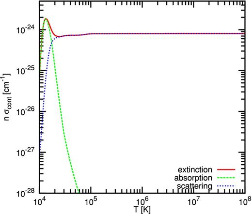
Variation of continuum opacity with temperature for a 1|$\mathrm{\thinspace cm}$| slab of unit hydrogen density. The contributions of absorption and scattering are also presented.
Because of our choice of unit density, numerically the continuum opacity is roughly equivalent to the extinction cross-section (to within a factor of a few). It follows that the inverse of the opacity amounts to the hydrogen column density required for τ ∼ 1. The largest value reported by Crawford et al. (2005) is not higher than 1022|$\mathrm{\thinspace cm^{-2}}$|. This indicates that gas hotter than 10 000|$\mathrm{\thinspace K}$| is optically thin to radiation at [Fe x].
Mittal et al. (2011) computed the gas-to-dust ratio through a 7|$\mathrm{\thinspace kpc}$| aperture to be at best 70. O'Dea et al. (1994) estimated the amount of molecular gas to ∼5 × 10⁸|$\mathrm{\thinspace \mathrm{M}_{\odot }}$| (see Mittal et al.), which we adopt here as the total mass for the molecular and dust components. This translates to a column density of ∼2 × 10²¹|$\mathrm{\thinspace cm^{-2}}$|. Combined with the declining absorption cross-section, we conclude that the cold matter in NGC 4696 is also optically thin to [Fe x].
Finally, extinction due to spectral lines is also negligible, as it is at most five orders of magnitude smaller than the continuum.
5 COMPARISON TO X-RAY GAS
Sanders et al. (2008) modelled their dispersive XMM–Newton spectra with cooling flow models and reported that no significant quantities of cool (≲0.4|$\mathrm{\thinspace keV}$|) gas were detected. Comparison with spatially resolved spectra obtained with Chandra (Sanders & Fabian 2006) indicates that the lowest temperatures arise from the central 30 arcsec, while higher temperatures are emitted progressively farther from the cluster centre. In fact, their best-fitting cooling flow models were consistent with mass deposition rates that diminish with decreasing temperature. An upper limit of 0.8|$\mathrm{\thinspace \mathrm{M}_{\odot } \, yr^{-1}}$| was obtained for their lowest temperature of 0.25|$\mathrm{\thinspace keV}$|. Similar results were obtained from spectral line analysis.
The coronal lines probe temperatures of 1–5 million K, and offer a complementary view into cooling at and beyond the softest bands accessible to X-rays. In order to constrain the state and origin of the coronal line gas, it is important to test whether it is consistent with being due to cooling from a possibly abated cooling flow.
For our analysis, we employ cloudy calculations that track a unit volume of gas at a hydrogen density of 0.07|$\mathrm{\thinspace cm^{-3}}$| as it cools from 80 million K to 10 000|$\mathrm{\thinspace K}$|, and ignore the transfer of the optically thin coronal lines. (Our results are not sensitive to the exact density value.) We adopt the abundances for the coolest of the five-component cooling flow model of Sanders et al. (2008) as the most appropriate for the question at hand, listed in the third column of Table 2.
Adopted elemental abundances relative to hydrogen in our simulations. The second column lists the solar abundances of Anders & Grevesse (1989). The last two columns list the abundances for the cool gas component obtained in the fits of Sanders et al. (2008): the five-component cooling flow model (third column) and the five-temperature thermal model (last column).
| Element | Solar | 5 × VMCFLOW | 5 × VAPEC |
|---|---|---|---|
| Nitrogen | 1.12E−4 | 3.93E−4 | 1.80E−4 |
| Oxygen | 8.51E−4 | 4.43E−4 | 4.00E−4 |
| Neon | 1.23E−5 | 9.84E−5 | 9.10E−5 |
| Magnesium | 3.80E−5 | 3.88E−5 | 3.46E−5 |
| Silicon | 3.55E−5 | 6.24E−5 | 5.68E−5 |
| Calcium | 2.29E−6 | 6.41E−6 | 5.96E−6 |
| Iron | 4.68E−5 | 5.05E−5 | 4.54E−5 |
| Nickel | 1.78E−6 | 4.52E−6 | 4.16E−6 |
Fig. 3 illustrates the ionization fractions of the relevant ions for both CIE and NEI isochoric calculations. Isobaric calculations produce identical results and are not shown. Evidently, in this temperature range, cooling and recombination are in equilibrium, in agreement with GS90 and Gnat & Sternberg (2007). The ionization fraction of Fe6 + is also presented to illustrate that non-equilibrium effects become important at lower temperatures.
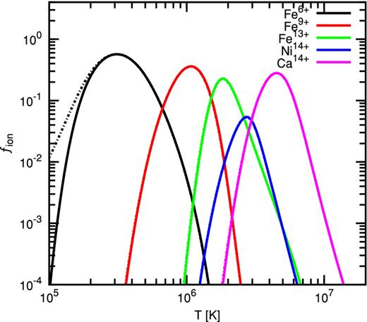
Fractional densities for the ions discussed by C11a, and for Fe6 +. Results are presented for both CIE (solid) and NEI (dashed) calculations of isochoric cooling. Recombination lags become significant below 2 × 10⁵|$\mathrm{\thinspace K}$|. The ions as listed in the legend proceed from left to right.
We begin by recalculating the mass deposition rate through [Fe x]. C11a reported that the luminosity in [Fe x] is 3.5 × 1037|$\mathrm{\thinspace erg \, s^{-1}}$|, which translates to |$\skew4\dot{M} \sim 1.63 \thinspace {\rm M}_{\odot } \, \mathrm{yr^{-1}}$|, given that Γ ≈ 3.42 × 10¹¹|$\mathrm{\thinspace erg \, g^{-1}}$| for isobaric cooling. (For isochoric cooling, Γ ≈ 2.07 × 10¹¹|$\mathrm{\thinspace erg \, g^{-1}}$| and the mass rate is ∼2.68|$\thinspace {\rm M}_{\odot } \, \mathrm{yr^{-1}}$|.) This is significantly lower than the rate of 20|$\thinspace {\rm M}_{\odot } \, \mathrm{yr^{-1}}$|, deduced by C11a using the older results of Sarazin & Graney (1991), and in overall agreement with the X-ray spectroscopy results. Note, however, that this estimate is in excess of the upper limit of 0.8|$\thinspace {\rm M}_{\odot } \, \mathrm{yr^{-1}}$| obtained by Sanders et al. (2008) by fitting the entire spectrum with a multicomponent cooling flow model.
In Table 3, we investigate the consistency of our cooling calculations against the cooling flow model predictions of Sanders et al. (2008, see table 3 therein). Following that work, our models cool from an initial temperature of ∼4.5|$\mathrm{\thinspace keV}$|. However, we do not employ solar metallicities as in that work, but instead use the abundances appropriate to their five-component VMCFLOW model as before. Note from Table 2 that the iron abundance is close to the solar value, while the nitrogen abundance is 3.5 times higher. We compute the Γ(T) functions for these lines and convert the X-ray luminosities to mass deposition rates with the aid of equation (4). Our calculations are in good agreement with the reported rates (shown in the last column of Table 3). N vii is the only exception because the adopted solar abundance in that paper is unrealistically low for the X-ray gas (see Sanders et al. for more details). Adjusting the reported mass deposition rate through N vii by 3.5 leads to a value comparable to the rate calculated by cloudy.
Updated mass deposition rates for the detected X-ray lines of Sanders et al. (2008) based on our isobaric calculations. For a more fair comparison, the integrations are done starting at a temperature of about 4.5|$\mathrm{\thinspace keV}$|. However, we do not assume solar metallicities. Instead, our results are drawn from calculations employing the abundances of their 5 × VMCFLOW model (see Table 2). The first two columns identify the X-ray emission line. The third column lists the reported line luminosity. The fourth column lists the Γ(T) functions, which are converted to mass deposition rates in the fifth column with the aid of equation (4). Finally, the last column shows the reported mass deposition rates for comparison.
| Label | λ/Å | L/1E+39 erg s−1 | Γ(T)/erg g−1 | |$\skew4\dot{M}_\mathrm{calc}$|/M⊙ yr−1 | |$\skew4\dot{M}_\mathrm{rep}$|/M⊙ yr−1 |
|---|---|---|---|---|---|
| Fe xvii | 15.01 | 12.4 | 1.23E+14 | 1.60 | 1.6 |
| Fe xvii | 15.26 | 3.6 | 3.32E+13 | 1.72 | 1.6 |
| Fe xvii | 16.78 | 4.3 | 6.13E+13 | 1.11 | 1.7 |
| Fe xvii | 17.05 | 19.3 | 7.64E+13 | 4.00 | 3.0 |
| N vii | 24.78 | 11.5 | 5.00E+13 | 3.65 | 9.7 |
Table 4 presents estimates for the mass deposition rate through the [Fe x] coronal line. These are obtained first by converting the ratio of X-ray to coronal luminosities into ratios of the mass deposition rates, and then by invoking the reported mass rates through the X-ray lines. The mass deposition rates cover the range 1–4|$\thinspace {\rm M}_{\odot } \, \mathrm{yr^{-1}}$|, in agreement with our estimate from the coronal line alone.
Coronal mass deposition rates based on the detected X-ray lines reported by Sanders et al. (2008). The first two lines identify the X-ray line. The third column lists the ratio of the X-ray luminosity to that of [Fe x] λ6375. The fourth column lists the ratio of the Γ(T) functions for a freely cooling gas (isochoric and isobaric cooling produce virtually identical ratios). The fifth column lists the ratio of mass deposition rates of the X-ray line relative to that of the coronal line, obtained with equation (4). The last column lists the mass deposition rate in the coronal line using the reported X-ray mass deposition rate, listed in the last column of Table 3.
| Label | λ/Å | L/L([Fe x]) | Γ(T)/Γ(T)([Fe x]) | |$\skew4\dot{M} / \skew4\dot{M}$|([Fe x]) | |$\skew4\dot{M}$|([Fe x])/M⊙ yr−1 |
|---|---|---|---|---|---|
| Fe xvii | 15.01 | 354 | 359 | 0.99 | 1.6 |
| Fe xvii | 15.26 | 103 | 97 | 1.06 | 1.5 |
| Fe xvii | 16.78 | 123 | 180 | 0.68 | 2.5 |
| Fe xvii | 17.05 | 551 | 224 | 2.46 | 1.2 |
| N vii | 24.78 | 329 | 146 | 2.25 | 4.3 |
This analysis indicates that the mass deposition rate through the coronal line is in reasonable agreement with the rates obtained from the X-ray lines. In principle, then, the coronal gas is consistent with cooling out of the hot ICM at a uniform rate in the range 1–10 million K. If that were the case, the expected luminosity for [Fe xiv] is about 1038|$\mathrm{\thinspace erg \, s^{-1}}$| or about twice the upper limit. (This result may be obtained by comparing to Fe xvii λ15.01 assuming a uniform deposition rate, and noting that for the coronal line Γ(T) = 5.9343 × 10¹¹|$\mathrm{\thinspace erg \, g^{-1}}$| for isochoric cooling.) The fact that the 2 million K [Fe xiv] line is not observed is perplexing.
6 CORONAL GAS AS A COOLING CONDENSATION
Deciphering the lack of any [Fe xiv] emission is fundamental to our understanding of the state of the coronal gas. If the coronal gas is indeed cooling out of the ambient ICM, the mass deposition rate through [Fe xiv] should be consistent with the X-ray and coronal line rates. We now leverage our cooling models to convert the upper limit to the luminosity ratio to a limit for the ratio of mass deposition rates.
Table 5 lists our estimates for the Γ(T) ratio between each of the undetected lines and the detected [Fe x]. They amount to the luminosity ratios expected for a simple cooling flow model of uniform deposition rate. Interestingly, the ratio of Γ(T) functions for [Fe xiv] is greater than the observed limit, suggesting that if the coronal gas was cooling freely from the hot ICM, the [Fe xiv] would probably have been observed.
Ratio of gamma functions, |$\Gamma _\mathrm{line} / \Gamma _\mathrm{[Fe\,\small {x}]}$|, for cooling calculations of the five-component cooling flow model of Sanders et al. (2008). The first two columns identify the spectral line, while the remaining columns list results for NEI and CIE cooling under isochoric (CD) and isobaric (CP) conditions.
| Spectral line | |||||
|---|---|---|---|---|---|
| Label | λ/Å | NEI–CP | CIE–CP | NEI–CD | CIE–CD |
| [Fe xiv] | 5303 | 2.84 | 2.84 | 2.85 | 2.87 |
| [Ca xv] | 5445 | 0.24 | 0.25 | 0.24 | 0.25 |
| [Ca xv] | 5695 | 0.56 | 0.57 | 0.56 | 0.58 |
| [Ni xv] | 6700 | 0.07 | 0.07 | 0.07 | 0.07 |
| Spectral line | |||||
|---|---|---|---|---|---|
| Label | λ/Å | NEI–CP | CIE–CP | NEI–CD | CIE–CD |
| [Fe xiv] | 5303 | 2.84 | 2.84 | 2.85 | 2.87 |
| [Ca xv] | 5445 | 0.24 | 0.25 | 0.24 | 0.25 |
| [Ca xv] | 5695 | 0.56 | 0.57 | 0.56 | 0.58 |
| [Ni xv] | 6700 | 0.07 | 0.07 | 0.07 | 0.07 |
6.1 Continuum subtraction
The C11a upper limits depend sensitively on the continuum subtraction method employed (see section 3.3 therein). In particular, single stellar population model spectra are dominated by stellar features below 6000 Å, which vary on scales comparable to the expected coronal line widths, complicating the analysis. C11a stress that the uncertainties in the stellar continuum subtraction may introduce a larger error into the reported upper limit for [Fe xiv].
We note that our calculations yield a Γ(T) function ratio of 2.85 for [Fe xiv] over [Fe x]. By contrast, the older models of GS90 predict values less than unity. This is a consequence of the changes in the [Fe xiv] λ5303 Å emissivity discussed in Section 3. In other words, our findings further exacerbate the non-detection of [Fe xiv].
While we acknowledge the complications involved in estimating accurate fluxes for the [Fe xiv] line, in the following, we assume that the non-detection is not due to such technicalities and explore its consequences for the state of the system.
6.2 Mass deposition rates
The maximum rates are presented in Table 6. Our calculations suggest that the mass deposition rate at a million K ([Fe x]) is twice as high as the rate at 2 million K ([Fe xiv]), or that more gas is cooling from a million K, than is cooling to that temperature. This contradicts cooling flow observations, which suggest that the mass deposition rate is either constant or increases with temperature.
| Spectral line | |||||
|---|---|---|---|---|---|
| Label | λ/Å | NEI–CP | CIE–CP | NEI–CD | CIE–CD |
| [Fe xiv] | 5303 | 0.45 | 0.45 | 0.45 | 0.45 |
| [Ca xv] | 5445 | 1.19 | 1.17 | 1.20 | 1.16 |
| [Ca xv] | 5695 | 1.94 | 1.90 | 1.96 | 1.89 |
| [Ni xv] | 6700 | 4.34 | 4.28 | 4.38 | 4.26 |
| Spectral line | |||||
|---|---|---|---|---|---|
| Label | λ/Å | NEI–CP | CIE–CP | NEI–CD | CIE–CD |
| [Fe xiv] | 5303 | 0.45 | 0.45 | 0.45 | 0.45 |
| [Ca xv] | 5445 | 1.19 | 1.17 | 1.20 | 1.16 |
| [Ca xv] | 5695 | 1.94 | 1.90 | 1.96 | 1.89 |
| [Ni xv] | 6700 | 4.34 | 4.28 | 4.38 | 4.26 |
| Spectral line | |||||
|---|---|---|---|---|---|
| Label | λ/Å | NEI–CP | CIE–CP | NEI–CD | CIE–CD |
| [Fe xiv] | 5303 | 0.45 | 0.45 | 0.45 | 0.45 |
| [Ca xv] | 5445 | 1.19 | 1.17 | 1.20 | 1.16 |
| [Ca xv] | 5695 | 1.94 | 1.90 | 1.96 | 1.89 |
| [Ni xv] | 6700 | 4.34 | 4.28 | 4.38 | 4.26 |
| Spectral line | |||||
|---|---|---|---|---|---|
| Label | λ/Å | NEI–CP | CIE–CP | NEI–CD | CIE–CD |
| [Fe xiv] | 5303 | 0.45 | 0.45 | 0.45 | 0.45 |
| [Ca xv] | 5445 | 1.19 | 1.17 | 1.20 | 1.16 |
| [Ca xv] | 5695 | 1.94 | 1.90 | 1.96 | 1.89 |
| [Ni xv] | 6700 | 4.34 | 4.28 | 4.38 | 4.26 |
The lack of any significant [Fe xiv] emission suggests that the coronal gas cannot have formed in situ as a cooling condensation of the surrounding ICM. It is more likely that, as the X-ray morphology suggests, the gas originated closer to the galactic nucleus, and it has been displaced to its current position by a dynamical process, such as uplifting by radio bubbles, and possibly heated. Other possibilities, such as conduction and mixing, are discussed in Section 9.
6.3 Differential extinction
Before we investigate the properties of the coronal gas in more detail, we explore the possibility that the lack of [Fe xiv] emission is due to extinction. Having established that the detected coronal line is optically thin, steep extinction laws are required to account for the observations.
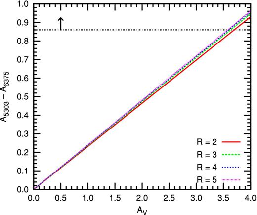
Dependence of differential extinction on the V-band extinction for a number of different R extinction laws. The dot–dashed line shows the limit derived from the observations for a Γ(T) ratio of 2.85 (see Table 6).
The required minimum extinction is difficult to reconcile with observations, as it exceeds the maximum V-band extinction estimates in the vicinity of NGC 4696. Sparks, Macchetto & Golombek (1989) reported a maximum of 0.4 at the south-western end of the dust lane, based on V- and R-band imaging. On the other hand, Farage et al. (2010) estimated a maximum of ∼0.7, 3 arcsec north-west of the nucleus, from the observed Hα/ Hβ ratio, and the standard assumption for active galaxies that its intrinsic value is higher than the Case B value, at 3.1. Canning et al. (2011b) reported maximum extinctions of AV ∼ 2–2.5 (see fig. B1 in their appendix) for a Case B Hα/ Hβ ratio. For values appropriate to active galaxies, however, they obtained results consistent with Farage et al. (2010). Similar results have been obtained by other authors (e.g. see references in Canning et al. 2011b).
In any case, there is not significant overlap between the gas cloud of interest (‘box 1’ in C11a) and regions of high extinction according to fig. B1 of Canning et al. (2011b), although C11a point out that assessing the connection between the coronal line gas and the optical filaments and dust lane will require deeper observations.
Also note that these conclusions are in qualitative agreement with the modelling of Werner et al. (2013). These authors postulated the presence of intervening cold absorbers intermixed with the X-ray filaments in Virgo, and found that a column density of 1.6 × 10²¹|$\mathrm{\thinspace cm^{-2}}$| may account for the lack of X-ray emission below 0.5|$\mathrm{\thinspace keV}$|. If a column density of that magnitude occurs in Centaurus as well, it would translate to reddening E(B − V) = 0.276, according to the dust-to-gas relation of Bohlin, Savage & Drake (1978), namely N (Hi + H2) = 5 × 10²¹ E (B − V). However, such a column can only account for the preferential extinction of the [Fe xiv], if the reddening constant has a value R ≳ 13. We can therefore rule out this possibility as well.
We conclude that extinction cannot account for the lack of [Fe xiv] emission.
6.4 Heating
Heating may prevent a gas from cooling to low temperatures either by establishing a temperature floor or by increasing the thermal energy of the gas and reducing its net cooling rate. Because the details of how heating affects gas at different temperatures are uncertain, simulations of the latter scenario fall beyond the scope of this paper. In this paper, we assume that heating, if it has occurred, has merely established a temperature floor. If the floor falls in the temperature range probed by [Fe x], it will affect the deduced mass deposition rates.
Fig. 5 explores the temperature dependence of the computed gamma ratios, as well as the maximum deposition rate ratios subject to the observed luminosity upper limits. The Γ(T) functions are computed between the initial temperature in the simulation and the temperature floor in question, T. In practice, an emission line contributes significantly over a limited temperature range. The range for the plots is chosen to cover most of the range probed by the [Fe x] line (see Fig. 1). At the left end of these plots, the Γ(T) and |$\skew4\dot{M}$| ratios are near the asymptote values shown in Table 6. At higher temperatures, the amount of cooling due to [Fe x] diminishes causing the Γ(T) ratios to increase and the mass deposition rate ratios to decrease.
![Left-hand panel: ratio of Γ(T, Tmax) for each of the non-detected lines against the detected [Fe x], as a function of temperature. Right-hand panel: maximum deposition mass rates for each of these lines, computed as the r.h.s. of equation (9), as a function of temperature.](https://oup.silverchair-cdn.com/oup/backfile/Content_public/Journal/mnras/446/2/10.1093_mnras_stu2173/2/m_stu2173fig5.jpeg?Expires=1750209439&Signature=pGrT60KAj31p0QeFyhlj0IXiUwLRjZLy7Z3legsUUmKqt9W1jVLVQr07TCgVy~jNHamghNn910TPaI0qCQMf13gdncZWf9URAHRehX9fE2F2ipCZZeMqB7AzLOK1qd2EhOSc1YpsRBZX8WJSAEPpgxqqcvRDHHUdZrAZFIP9Ze3FYHjpmnvosqdf37DNLPJphDaula~4qHQmWOyFhVwzYjmtlvzr4KM1hvlN6cyg2TCwkFy7O5TAvcwbZ36IWl2Nlu1TKtg4U8b7RNoMkKvg2W3Rgz59k5rbYdEd7P8j5nTIHaK-ZEazRHyRFxxsvoSBV35lIdHn4SQgKM3zwKcBjg__&Key-Pair-Id=APKAIE5G5CRDK6RD3PGA)
Left-hand panel: ratio of Γ(T, Tmax) for each of the non-detected lines against the detected [Fe x], as a function of temperature. Right-hand panel: maximum deposition mass rates for each of these lines, computed as the r.h.s. of equation (9), as a function of temperature.
It is important to notice that the Γ(T) ratio for [Fe xiv] is always higher than unity, suggesting that cooling due to this line is more important than cooling due to the [Fe x] over the entire temperature range. This is partly because the gas cools faster through the temperature range probed by [Fe x].
The right-hand panel of Fig. 5 illustrates that the mass deposition rate consistent with the observed upper limits for [Fe xiv] is always lower than the rate traced by [Fe x]. In fact, the rate becomes progressively lower at higher temperatures, as the cooling due to [Fe x] diminishes. If extinction is at work, even higher values than previously computed are required to account for the increasing Γ(T) ratios.
These arguments show that a simple temperature floor cannot account for the lack of emission from gas hotter than ∼million K in the observations of C11a, and support our conclusion that the coronal gas cannot be a cooling condensation of the surrounding ICM.
7 CONSTRAINTS FROM [Fe xiv]
As discussed in Section 8, constraining the properties of the coronal gas requires an estimate of the volume it occupies. The coronal gas was detected along the cool X-ray plume (Sanders & Fabian 2002), and most likely it is embedded within the X-ray filament. However, the connection between the X-ray and coronal phases, as well as the optical filaments, remains unclear (C11a).
In this section, we consider the possibility that the coronal gas is projected on to the X-ray cool filament by chance, and arrive at an estimate for its volume fraction. For this purpose, we assume that gas cooling may be described by the cooling flow formalism, in the sense that line luminosities are given by equation (4). Because cooling is thought to occur ‘locally’, we take the mass deposition rate to be constant. Differences in the cooling rate are encapsulated in the Γ(T) function and fully accounted for when taking line ratios. We also adopt the abundances of the 5 × VAPEC model fits of Sanders et al. (2008), as shown in the last column of Table 2. Note, however, that the differences to the abundances appropriate to the five-component cooling flow model are within the statistical errors (10 per cent) for most elements.
7.1 Temperature ceiling
We consider the luminosity ratio between the [Fe xiv] and [Fe x] lines computed over the temperature intervals which contribute 99 per cent of the respective total line luminosity. Our goal is to obtain an estimate for the maximum temperature of the coronal gas that is consistent with the reported upper limit ([Fe xiv]/[Fe x] <1.29). We let the maximum temperature of the gas vary between the temperature at which the cooling efficiency of [Fe xiv] peaks (1.8 million K) and the upper end of the line temperature range. We also explore the robustness of these calculations in the presence of a temperature floor, which we simulate by letting the minimum temperature probed by [Fe x] be at most equal to the temperature of peak cooling efficiency (∼1 million K) and no less than the lower end of the line temperature range. (The temperature range probed by [Fe x] is |$T^X_\mathrm{min} \le T \le T^X_\mathrm{max}$|.) Fig. 6 shows that the computed luminosity ratio is consistent with the reported upper limit for temperatures no greater than 2.1 million K. This is true for both isochoric and isobaric cooling. The presence of a temperature floor does not modify these results significantly. In the following, we adopt a conservative temperature ceiling of 2.1 million K.
![Ratio of the computed luminosity ratio of [Fe xiv] over [Fe x] in units of the reported upper limit (1.29). The results shown are for isobaric cooling. The temperature ceiling varies along the x-axis, while the temperature floor varies along the y-axis. The upper limit is consistent with a temperature ceiling of ∼2.1 million K.](https://oup.silverchair-cdn.com/oup/backfile/Content_public/Journal/mnras/446/2/10.1093_mnras_stu2173/2/m_stu2173fig6.jpeg?Expires=1750209439&Signature=N88XvqFSwnh3bzqfA0s25HP~vmsi6mQmErsr6qsJXXU62x13US7~wnhJGIPahx9LXLR2vWJMWXQGldPIi7d1ix2je9FEptjPAKYEOL0FOxoNBJu6vMda0gORLEH20Gpu~S0oAdJzgIK6qMpWe9vn61D7exGSqMC23HjdxBn2WaTS9~yO04XI1EIoyvIaOFAOtCRaVyRIqc0akl5N3S0tGe6PUPy0J786icqQpY-ghlPL9lb1aJYPk5b-4nsibk8hIay5hYsPwIJBM36tvHBJNQ9-f1ue5uzZMVyI4sRlvV6r8kB2VPSkKfsOXFPt~KZU6fjDsYdF0AEq~5vtTjmKjg__&Key-Pair-Id=APKAIE5G5CRDK6RD3PGA)
Ratio of the computed luminosity ratio of [Fe xiv] over [Fe x] in units of the reported upper limit (1.29). The results shown are for isobaric cooling. The temperature ceiling varies along the x-axis, while the temperature floor varies along the y-axis. The upper limit is consistent with a temperature ceiling of ∼2.1 million K.
7.2 Volume filling factors
We compute the volume fraction of the [Fe x] phase as a function of the temperature floor, which we let extend to 10 000|$\mathrm{\thinspace K}$|. The integration in the numerator of equation (12) is carried out over the range |$(T, T^X_\mathrm{max})$|, where |$T \ge T^X_\mathrm{min}$|. In the denominator, the integration is carried out over (T, Tmax), where Tmax is the adopted temperature ceiling. As Fig. 7 shows, typical values are in the range of 50–75 per cent. For isobaric cooling, the volume fraction obtains an asymptotic value at low temperatures, due to compression. For isochoric cooling, by contrast, the volume fraction declines with decreasing temperature below 200 000|$\mathrm{\thinspace K}$|. The NEI calculations predict a slightly lower volume fraction. This is due to reduced cooling relative to CIE (Gnat & Sternberg 2007), which leads to gas surviving for longer at such temperatures.
![Volume fraction of the phase that emits [Fe x] as a function of the temperature floor. The calculations are done for temperatures below the cooling efficiency peak. The line cooling efficiency effectively drops to zero below 0.55 million K.](https://oup.silverchair-cdn.com/oup/backfile/Content_public/Journal/mnras/446/2/10.1093_mnras_stu2173/2/m_stu2173fig7.jpeg?Expires=1750209439&Signature=3t6-NO5U5Ib7JtexURDr6HwDnZRK24~vm92iqfb6PUTFV25Phh~4iF0gdqHZXH2K3ZorUVU94wEN55lCHyQZ2vPbP7clFrsufhQvtHbHstmxoGlyxx-b8CESTkArXkIOd8MywG0il~1iiqRfIl5lNXLwkjU5AUSxYlbPkip4CnOaHhMusv0r-jjEQB8svA3InWm0K6-GdDljnG~MSrQw9Mrypsn6632SRfIrDL-1sgA6-qTE0OMuvzcoiwWUzRzI9hK~z0dRcY9aJygQL~dbze~~ix1NN9REsJKtp0GZwadJ0WvMsqtjrxhGngp3jVTK3~uUqxRYeiEnszSmjHmqpw__&Key-Pair-Id=APKAIE5G5CRDK6RD3PGA)
Volume fraction of the phase that emits [Fe x] as a function of the temperature floor. The calculations are done for temperatures below the cooling efficiency peak. The line cooling efficiency effectively drops to zero below 0.55 million K.
8 CORONAL GAS PROPERTIES
The [Fe x] luminosity may be used to infer the coronal gas properties. Motivated by the optical and X-ray filaments in the same region, we approximate the coronal gas as a cylinder and take its diameter and height equal to the size reported by C11a, i.e. 2R ∼ 700|$\mathrm{\thinspace pc}$|. Below, we first explore the scenario that the coronal gas is independent of the X-ray plume, and then that it is embedded within the plume.
8.1 Independent structure
All cooling runs are consistent with a hydrogen density of ∼0.2|$\mathrm{\thinspace cm^{-3}}$|. This includes isochoric and isobaric calculations, in and out of collisional equilibrium. The obtained density is not sensitive to the adopted volume fraction, |$n_{\rm H} \propto f_{\rm V}^{-1/2}$|, and values in the range 50–75 per cent lead to small density variations. The coronal gas mass is about 1.5 × 10⁶|$\mathrm{\thinspace \mathrm{M}_{\odot }}$|.
If we assume that the coronal gas is thermally supported, pressure equilibrium translates to a distance of the cloud to the radio source of about 20|$\mathrm{\thinspace kpc}$|. However, C11a concluded that the [Fe x] is turbulently broadened at ∼300|$\mathrm{\thinspace km \, s^{-1}}$|. We have therefore assumed that transonic turbulence (υturb ∼ cs, where υturb is the turbulent velocity and cs is the sound speed) contributes to the pressure budget of the coronal cloud. This leads to a line width of ∼250|$\mathrm{\thinspace km \, s^{-1}}$|, in decent agreement with the observations. Pressure equilibrium, then, translates to a distance of ∼8|$\mathrm{\thinspace kpc}$|, suggesting that the X-ray arc is located within NGC 4696. The projected distance from the nucleus is ∼3|$\mathrm{\thinspace kpc}$|, so the line-of-sight distance to the nucleus is ∼7.5|$\mathrm{\thinspace kpc}$|.
The sound crossing time of the coronal cloud is about 4.5|$\mathrm{\thinspace Myr}$|. By contrast, the gas cooling time is ∼0.6|$\mathrm{\thinspace Myr}$| for isochoric cooling and ∼0.8|$\mathrm{\thinspace Myr}$| for isobaric cooling. In either case, the cooling time is a small fraction of the crossing time, which suggests that the gas cooling proceeds under conditions of constant density (isochoric).
In cooling flow models, the gas is cooling such that its temperature follows the underlying gravitational potential (McNamara & Nulsen 2007). This property allows one to test for the possibility that the gas has been displaced to the observed location. An alternative method is to compare the entropy content of the coronal gas to that of the surrounding ICM, as described by the fitting forms of Graham et al. (2006). Note that the ICM follows the familiar K(r) ∝ r0.96 entropy law down to ∼1|$\mathrm{\thinspace kpc}$| from the nucleus. We find that the coronal gas carries about 1/90 of the entropy in the surrounding X-ray gas. If the entropy distribution holds at sub-kpc scales, the coronal gas entropy is consistent with a distance of ∼0.1|$\mathrm{\thinspace kpc}$| from the nucleus, and therefore consistent with a displacement scenario.
8.2 Embedded in X-ray plume
If the coronal gas is embedded within the X-ray plume, we can require that it be in pressure equilibrium with the hot phase, and we can use the coronal luminosity to constrain its volume fraction.
9 DISCUSSION
Our analysis indicates that the coronal gas is a young dynamical feature in NGC 4696. It is unlikely that it has cooled out of the surrounding ICM, or [Fe xiv] would have been observed. Yet, it coincides with the X-ray cool filament in projection, which suggests that the two phases may in fact be co-spatial. The coincidence with the optical filaments is more tenuous and requires further investigation (C11a).
If the optical and coronal phases are not related to each other, the coronal gas could possibly have originated as warm (∼104|$\mathrm{\thinspace K}$|) gas that was vigorously heated, and in which cooling has recently been re-established. The energy required to heat the coronal gas from 104 to 106|$\mathrm{\thinspace K}$| is 4 × 1053|$\mathrm{\thinspace erg}$|. According to Taylor et al. (2006), the power of the AGN of NGC 4696 is currently <1040|$\mathrm{\thinspace erg \, s^{-1}}$|, which suggests that the AGN outburst lasted at least 1.5 million years. These calculations assume 100 per cent efficiency and do not account for the work required to lift the gas out to 9|$\mathrm{\thinspace kpc}$|, so likely the outburst lasted longer and/or was more powerful. The time-scale is plausible, as it is comparable with the ∼2.5|$\mathrm{\thinspace Myr}$| periodicity of the AGN in M87 (Nulsen et al. 2007). Higher final temperatures (>106|$\mathrm{\thinspace K}$|) require higher outburst powers, durations, or both. However, this scenario is not satisfactory, because it requires some fine-tuning in order to account for the fact that we get to observe freely cooling gas of such short cooling time.
A more natural explanation would involve the coronal gas as a phase of a steady-state system. Most likely the optical, coronal, and X-ray phases are related to each other. Then, the coronal gas may be the conductive or mixing interface between the optical, 104|$\mathrm{\thinspace K}$|, filaments and the cool X-ray gas, 107|$\mathrm{\thinspace K}$|. Examples of conductive interfaces in rough agreement with the coronal gas properties may be found in Boehringer & Fabian (1989). On the other hand, Begelman & Fabian (1990) present crude estimates on the structure of mixing layers. The temperature distribution of the gas in the mixing layer is analytically unknown. The geometric mean temperature is around 300 000|$\mathrm{\thinspace K}$|, subject to unknown, order-of-unity efficiency factors. This is effectively consistent, to within a factor of a few, with the temperature of the [Fe x] gas. In addition, assuming that the ambient ICM is turbulent, and that the turbulent velocity is close to the sonic speed, we obtain from their equation 2 that the depth of the mixing layer is roughly 1.3|$\mathrm{\thinspace kpc}$|, consistent with the X-ray filament width to a factor of 2. Based on the sharpness of the optical filaments (Crawford et al. 2005), the ICM is thought to not be particularly turbulent, which should improve the agreement with the observations. In fact, plugging in that equation the previous estimate of ∼90|$\mathrm{\thinspace pc}$| for the thickness of the mixing layer, we obtain highly subsonic turbulent motions in the plume, such that |${\cal M} < 0.1$|.
Note that in the simulations of Esquivel et al. (2006), which do not parameterize uncertainties with efficiency factors, the mixing layer that forms between the 104 and 107|$\mathrm{\thinspace K}$| phases has a density-weighted temperature of 1–2 million K. However, these simulations do not reach steady state after 3|$\mathrm{\thinspace Myr}$| of integration and do not include the effects of NEI. The more recent simulations of Kwak & Shelton (2010) do include non-equilibrium effects, albeit in an idealized two-dimensional, unmagnetized setting. They find that in the simulation most similar to our case (Model F, which has a hot-phase temperature of 3 × 10⁶|$\mathrm{\thinspace K}$|), the mixing layer does not reach steady state by the end of their runs (80 Myr), unlike simulations at lower temperatures for the hot phase. However, they point out that the rate of growth for the mixing layer correlates with the shear speed. This suggests that higher shear speeds may be required to produce a steady-state mixing layer in the X-ray plume.
Signatures of gas at intermediate temperatures may help resolve the state and origin of the coronal gas. Obviously, conduction and mixing models involve multitemperature gas distributions, so detection of emission lines from intermediate temperature may be expected. Such emission lines have been observed previously in Virgo, where C iv λ1549 due to 105|$\mathrm{\thinspace K}$| has been reported by Sparks et al. (2009, 2012). Or, in Abell 426 and Abell 1795, where gas at 105.5|$\mathrm{\thinspace K}$| gives rise to O vi λλ 1032, 1038 Å (Bregman et al. 2006). In Fig. 8, we present the best candidate lines identified in our cooling simulations. These lines are brighter than the detected [Fe x], also shown. The evolution with time and temperature indicates that some of these lines although very bright are associated with gas of short cooling time, and may not be easily detected. However, if the coronal gas is cooling in a steady state, some of these lines will likely be observable in the ultraviolet.
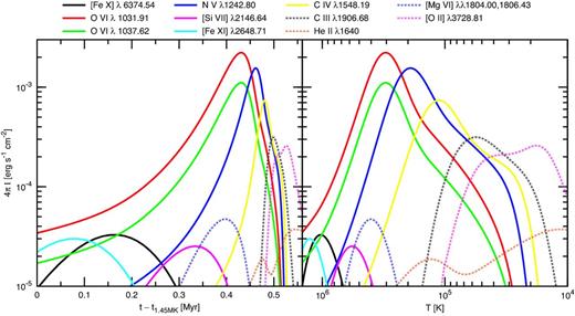
Intensity of various lines produced by a gas column as a function of time (left) and decreasing temperature (right) for our cooling calculations. The column length is equal to the coronal cloud diameter and the hydrogen density is set to 0.2|$\mathrm{\thinspace cm^{-3}}$|. Time is measured since the moment when the temperature is 1.45 million K.
The non-detection of either [Fe x] or [Fe xiv] in the north-west end of the X-ray arc poses difficulties to the mixing and conduction scenarios. The north-west end of the arc lies close to the dust lane, so absorption is a likely cause for the non-detections, without requiring fine-tuning of the obscuring column density. Alternatively, or in addition, if that gas lies deeper into the potential well, the mean temperature of the mixing layer may be lower than that at the south-east end, which would diminish emission from ∼million K gas.
It is also possible that the differences between the two regions are the result of rapid cooling. Non-uniformities in the density field or in the heating mechanism may accentuate differences in cooling across the X-ray plume and lead to a more clumpy gas distribution (as in, e.g. Nulsen 1986). Indeed, the granularity of the sub-keV gas around NGC 4696 (see fig. 1 in C11a) is reminiscent of a collection of clouds.
On the other hand, Panagoulia, Fabian & Sanders (2013) reported recently a significant drop in iron abundance within 5–10|$\mathrm{\thinspace kpc}$| of the nucleus in NGC 4696, which is of the order of a few relative to the more remote (say 20|$\mathrm{\thinspace kpc}$|) ICM. The possibility that the north-west region observed by C11a lies within the depleted region would provide a natural explanation to the absence of any detectable coronal iron emission. It would also require that the X-ray plume is elongated along the line of sight, so that the south-east region lies farther out, and is not drastically affected by the abundance drop.
10 SUMMARY
We have employed self-consistent non-equilibrium cooling calculations implemented in cloudy to study the thermal properties of the coronal line gas near the core of NGC 4696. The non-detection of the [Fe xiv] line suggests that the coronal cloud is not a cooling condensation of the surrounding ICM. Fine-tuned values of intrinsic extinction would be required to explain the detection of the optically thin [Fe x], but not of [Fe xiv].
The failure to detect [Fe xiv] suggests a temperature ceiling for the coronal cloud, which we estimate at ∼2.1 million K. This result is not sensitive to the presence of a temperature floor. The coronal gas is likely embedded in the X-ray plume, but even if it is not, it cools isochorically and its mass is ∼million M⊙.
Finally, we have briefly explored a few scenarios for the origin of the coronal cloud, and we have pointed out that the cloud is consistent with being either the conductive or the mixing interface between the hot ICM and the warm optical gas. Detailed calculations for observable signatures of these models are beyond the scope of the paper. None the less, we have presented a number of bright lines that trace gas down to 104|$\mathrm{\thinspace K}$|.
We would like to thank Orly Gnat and Matthias Steffen for valuable assistance with the validation of the time-dependent scheme in cloudy. GJF acknowledges support by NSF (0908877, 1108928, and 1109061), NASA (10-ATP10-0053, 10-ADAP10-0073, and NNX12AH73G), JPL (RSA No 1430426), and STScI (HST-AR-12125.01, GO-12560, and HST-GO-12309). ACF thanks European Research Council for the Advanced Grant FEEDBACK. PvH acknowledges support from the Belgian Science Policy Office through the ESA PRODEX programme.
Contains material © British Crown copyright 2011/MoD.
Enabled with the command set cumulative mass.
Enabled with the command set cumulative flux.
REFERENCES
APPENDIX A: cloudy INPUT
As a means to reproduce our results, we provide a minimal input script for isobaric cooling in CIE.
coronal 8e7 K init time
set dynamics population equilibrium
iterate to convergence
stop time when temperature falls below 1e4 K
c
atom chianti ``CloudyChiantiAll.ini''
hden 1 linear
constant gas pressure reset
c
set dr 0
set zone 1
