


Abstract
The non-linear, scale-dependent bias in the mass distribution of galaxies and the underlying dark matter is a key systematic affecting the extraction of cosmological parameters from galaxy clustering. Using 95 million haloes from the Millennium-XXL N-body simulation, we find that the mass bias is scale independent only for k < 0.1 h Mpc−1 today (z = 0) and for k < 0.2 h Mpc−1 at z = 0.7. We test analytic halo bias models against our simulation measurements and find that the model of Tinker et al. is accurate to better than 5 per cent at z = 0. However, the simulation results are better fitted by an ellipsoidal collapse model at z = 0.7. We highlight, for the first time, another potentially serious systematic due to a sampling bias in the halo velocity divergence power spectra which will affect the comparison between observations and any redshift-space distortion model which assumes dark matter velocity statistics with no velocity bias. By measuring the velocity divergence power spectra for different sized halo samples, we find that there is a significant bias which increases with decreasing number density. This bias is approximately 20 per cent at k = 0.1 h Mpc−1 for a halo sample of number density |$\bar{n} = 10^{-3} (h/$| Mpc)3 at both z = 0 and 0.7 for the velocity divergence auto power spectrum. Given the importance of redshift-space distortions as a probe of dark energy and the major ongoing effort to advance models for the clustering signal in redshift space, our results show that this velocity bias introduces another systematic, alongside scale-dependent halo mass bias, which cannot be neglected.
1 INTRODUCTION
Current and upcoming galaxy surveys such as BOSS (Schlegel et al. 2007), DES (Frieman & Dark Energy Survey Collaboration 2013), DESI (Levi et al. 2013), LSST (Ivezic & the LSST Collaboration 2008) and Euclid (Laureijs et al. 2010) will require extremely accurate theoretical predictions to match the precise observations of large-scale structure in our Universe. Cosmological N-body simulations which combine high resolution and large volume have the statistical power to play a key role in guiding the development of accurate theoretical models which will advance our understanding of the hierarchical growth of structure, galaxy formation and the properties of dark energy. A large uncertainty in extracting cosmological information from observations is the bias between galaxies or dark matter haloes and the underlying dark matter distribution. Using the Millennium-XXL (MXXL) simulation of Angulo et al. (2012), we examine both the halo mass and velocity bias for different mass bins and compare with theoretical predictions. To our knowledge, this is the first time that the velocity divergence power spectra have been presented for haloes of different masses measured from N-body simulations. Accurate models for the mass and velocity bias of haloes are extremely important in theoretical predictions for redshift-space distortions which are a major cosmological probe in the Dark Energy Task Force stage IV experiments (Albrecht et al. 2006).
Dark matter haloes form at high fluctuation peaks in the matter distribution and represent a biased tracer of the dark matter (e.g. Bardeen et al. 1986). As a consequence, extracting cosmological parameters from clustering statistics requires an accurate model for this bias as a function of both scale and redshift (e.g. van den Bosch, Mo & Yang 2003; Cole et al. 2005). Previous studies have calibrated semi-analytic models for the halo mass bias from simulations using either a friends-of-friends (FOF) halo finding algorithm (Jing 1998; Sheth, Mo & Tormen 2001; Seljak & Warren 2004; Tinker et al. 2005; Pillepich, Porciani & Hahn 2010) or a spherical overdensity (SO) halo finder (Hu & Kravtsov 2003; Manera, Sheth & Scoccimarro 2010; Tinker et al. 2010). In the FOF approach, particles are simply linked together in a percolation scheme which tracks iso-density contours. The main advantage of this method is that it makes no assumptions about halo geometry and tracks the shapes of bound objects faithfully. In the SO approach, haloes are identified as isolated spheres around density peaks where the mass of a halo is defined by the overdensity relative to the background. Simulations have shown that the mass function and bias for FOF and SO defined haloes can differ substantially at the high-mass end where the FOF algorithm tends to spuriously group distinct haloes together (Lukić et al. 2009; Tinker et al. 2010). Recent analytical advancements to the excursion set theory of halo formation which accounts for both non-Markovian walks and stochastic barriers have been developed (Maggiore & Riotto 2010) but have yet to be rigorously tested or calibrated against simulations. In this paper, we re-visit some of these models and compare their predictions with the measured bias for FOF haloes in the MXXL simulation at z = 0 and 0.7 for a much wider range of halo masses than previously explored at both redshifts (e.g. Angulo et al. 2008).
Okumura & Jing (2011) carried out a detailed analysis of the redshift-space clustering of dark matter haloes and the systematic effects on measuring the growth rate parameter taking into account uncertainties in the halo mass bias. Recent advancements in modelling redshift-space distortions, where the apparent positions of galaxies are altered along the line of sight by their intrinsic velocities (Kaiser 1987), have shown that taking into account non-linearities in the velocity field provides an improved model for the power spectrum on quasi-linear scales (Scoccimarro 2004; Jennings, Baugh & Pascoli 2011; Jennings et al. 2012). These studies focused on the redshift-space distortion effects in the dark matter only and assume that halo velocities trace the dark matter velocity field faithfully.
Here, we present, for the first time, the halo velocity divergence power spectra for different halo mass bins and show that there is a significant sampling bias compared to the dark matter velocity power spectrum. Measuring the velocity field from simulations has been shown to be extremely sensitive to resolution effects (Pueblas & Scoccimarro 2009; Jennings et al. 2011). The high force and mass resolution in the MXXL simulation allows us to accurately probe the extent of this velocity bias for different halo masses as a function of scale, redshift and number density. This has not been possible before for such a broad range of halo masses. Accounting for and modelling this bias in improved redshift-space distortion models is left to future work.
The attainable precision of cosmological parameters extracted from clustering statistics is also limited by the galaxy shot noise which is often modelled using Poisson statistics. Following the work of Seljak, Hamaus & Desjacques (2009), we investigate if a mass-dependent weighting of the density field can be used to suppress the shot noise in the clustering signal of high-mass haloes compared to the Poisson signal. This method relies on the assumption that on large scales the halo or galaxy cross-correlation coefficient is unity assuming a deterministic relationship between the dark matter and halo density fields.
The mxxl simulation (Angulo et al. 2012) is one of the largest high-resolution cosmological simulations to date, employing over 300 billion particles to model the evolution of the matter distribution in a volume of almost 70 Gpc3. The MXXL run complements previous simulations of the same cosmology in different box sizes with different particle numbers, the Millennium and Millennium-II simulations (Springel et al. 2005; Boylan-Kolchin et al. 2009). At present, the largest simulations carried out, such as the MICE Grand Challenge (Fosalba et al. 2013) of 70 billion dark matter particles in a (3 h−1 Gpc)3 comoving volume, the Dark Energy Universe Simulation Full Universe Run (Alimi et al. 2012) of 550 billion particles in a (21 h−1 Gpc)3 comoving volume, the MultiDark simulation (Prada et al. 2012) of ∼57 billion particles in a (2.5 h−1 Gpc)3 comoving volume, the DarkSky simulation (Skillman et al. 2014) of ∼107 billion particles in a volume 8 h−1 Gpc on a side or the Horizon Run 3 simulation (Kim et al. 2011) of 375 billion particles in (10.8 h−1 Gpc)3 comoving volume, cannot match the mxxl simulation in both mass and force resolution, which allows us to accurately model halo masses and velocities from 1012 to 1015 h−1 M⊙ over a range of redshifts.
Note two recent studies by Baldauf, Desjacques & Seljak (2014) and Zhang, Zheng & Jing (2014) have also reported that there should be a bias in the velocity power spectra. Baldauf et al. (2014) measure the velocity field directly from N-body simulations and detect a significant velocity bias for dark matter haloes as a function of redshift. Zhang et al. (2014) present theoretical modelling for sampling artefacts in volume-weighted velocity divergence power spectra using a nearest-particle velocity assignment method. In this work, we present measurements of the velocity divergence power spectrum obtained using both mass- and volume-weighted methods and quantify the impact of these sampling artefacts on different halo number densities at different redshifts. Although we analyse a different statistic using very different assignment methods, our results agree with the measurements of Baldauf et al. (2014) and the theoretical predictions of Zhang et al. (2014).
This paper is organized as follows: in Section 2, we describe the mxxlN-body simulation used in this paper. In Section 3, we analyse the halo matter power spectra for different mass bins at redshifts z = 0 and 0.7. These redshifts are chosen to be relevant to current and future redshift surveys. The z = 0.7 results presented here are directly relevant for the targets for Euclid (z = 0.5–2; Laureijs et al. 2010) and eBOSS spectroscopy which will consist of luminous red galaxies (LRG: 0.6 < z < 0.8) and emission-line galaxies (ELGs: 0.6 < z < 1.0); prime focus spectrograph (Takada et al. 2014) targets of [O ii] ELGs extending over the redshift range 0.8 < z < 2.4 and DESI (Levi et al. 2013) LRG and ELG targets refined to probe the z > 0.6 epochs at higher resolution than eBOSS.
We compare the measured linear bias from the MXXL simulation to different models for the bias at both redshifts. In Section 3.2, we examine whether the shot noise for a high-mass sample of haloes can be reduced using a mass-weighting method compared with Poisson shot noise estimates. In Section 4, we present the measured velocity divergence power spectra for the different mass bins measured from the mxxl simulation at redshifts z = 0 and 0.7 and compare with theoretical models for the dark matter velocity field. Our conclusions and summary are presented in Section 5.
2 THE MXXL N-BODY SIMULATION
The MXXL simulation follows the evolution of the matter distribution within a cubic region of 4.11 Gpc (3 h−1 Mpc) on a side using 67203 particles (see Angulo et al. 2012, 2014, for full details). The simulation volume is equivalent to that of the full sky out to redshift 0.7. The MXXL run particle mass is mp = 8.456 × 10⁹ h−1 M⊙. The MXXL adopts the same Λ cold dark matter (ΛCDM) cosmology as in the simulations presented in Springel et al. (2005) and Boylan-Kolchin et al. (2009), which facilitates the use of all three simulations for comparative studies of galaxy formation in simulations. The cosmological parameters of the simulation are Ωm = 0.25, Ωb = 0.045, ΩΛ = 0.75, σ8 = 0.9 and H0 = 73 km s−1 Mpc−1. Although the power spectrum normalization σ8 is somewhat high compared to current estimates (Komatsu et al. 2010), the theoretical models for the halo bias and velocity statistics considered in this work have previously been tested using simulations of varying cosmologies (Jennings et al. 2010; Tinker et al. 2010). Given the impressive mass and force resolution in the MXXL simulation, it is interesting to test the validity of these models for halo masses which lie beyond the resolving power of the original simulations used for calibration. The mxxl simulation was run using a ‘lean’ version of the gadget-3 code which is a highly optimized version of the TreePM code gadget-2 (Springel 2005; Springel et al. 2005). The group finder makes use of an FOF algorithm (Davis et al. 1985) to locate gravitationally bound structures.
3 THE SPATIAL DISTRIBUTION OF DARK MATTER HALOES
In this section, we present the measured power spectra of various halo mass samples from the MXXL simulation at z = 0 and 0.7. We focus first on comparing the halo power spectrum with that of the matter distribution, as quantified through the halo mass bias (Section 3.1). We then test a prescription for suppressing the shot noise in the power spectrum of a halo sample which is a modification of the method proposed by Seljak et al. (2009, section 3.2).
3.1 Bias of dark matter haloes
We analyse the linear bias measured from the ratio of the halo auto and mass power spectra b ≡ (Phh/Pm)1/2 as a function of scale and compare the predictions for the bias–peak height relation with commonly used models. The power spectrum was computed by assigning the particles to a mesh using the cloud-in-cell (CIC) assignment scheme (Hockney & Eastwood 1981) and then performing a fast Fourier transform on the density field. To restore the resolution of the true density field, this assignment scheme is corrected for by performing an approximate de-convolution (Baumgart & Fry 1991). Throughout this paper, the fractional error on the power spectrum plotted is given by |$\sigma _{\rm P}/P = (2/N)^{1/2}(1 + \sigma _n^2/P)$|, where N is the number of modes measured in a spherical shell of width δk and σn is the shot noise (Feldman, Kaiser & Peacock 1994). This number depends upon the survey volume, V, as N = V4πk2δk/(2π)3.
In Fig. 1, we show the z = 0 halo power spectra for the halo samples listed in Table 1. The dark matter power spectrum is shown as a purple solid line in this figure. In the middle panel, we show the halo bias at z = 0 for each halo sample evaluated as |$b = \sqrt{P_{\rm hh}/P_{{\rm m}}}$|. The best-fitting value for the bias over the range 0.004 < k(h Mpc−1) < 0.1 is shown as horizontal lines for each sample. These ratios are remarkably flat over the range k < 0.2 h Mpc−1 for masses <2 × 10¹³ h−1 M⊙ and k < 0.1 h Mpc−1 for masses >6 × 10¹³ h−1 M⊙ at z = 0 in agreement with the work of Okumura & Jing (2011). At a higher redshift of z = 0.7 shown in Fig. 2, this bias is scale independent for all masses at k < 0.1 h Mpc−1 although the scale dependence is more pronounced on quasi-linear scales compared to redshift zero.
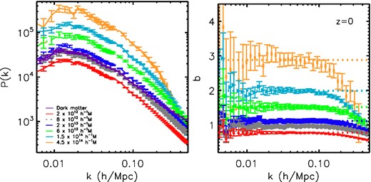
Left: the halo power spectra for different halo mass ranges measured from the MXXL simulation at z = 0. Note that not all error bars are plotted after k = 0.06(0.02)h Mpc−1 in the left-hand (right-hand) panel for clarity. Right: the z = 0 measured halo bias for different mass ranges where |$b = \sqrt{P_{\rm hh}/P_{{\rm m}}}$|. The horizontal lines in each case represent the best-fitting value for the bias over the range k < 0.1 h Mpc−1.
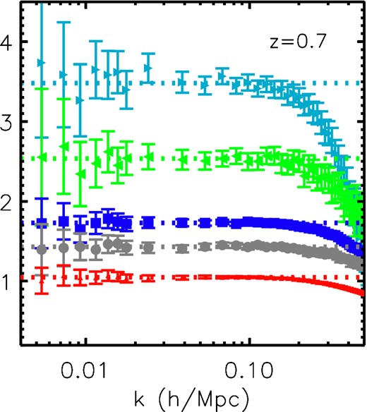
The halo bias measured at z = 0.7. The colour coding for each mass bin is given by the legend in the left-hand panel of Fig. 1.
| Mass range | Number density | (h/Mpc)3 |
|---|---|---|
| (h−1 M⊙) | z = 0 | z = 0.7 |
| >1 × 10¹² | 3.54 × 10⁻³ | – |
| 1–3 × 10¹² | 2.26 × 10⁻³ | 2.27 × 10⁻³ |
| 7–9 × 10¹² | 1.22 × 10⁻⁴ | 1.07 × 10⁻⁴ |
| 1–3 × 10¹³ | 2.47 × 10⁻⁴ | 1.96 × 10⁻⁴ |
| 5–7 × 10¹³ | 2.38 × 10⁻⁵ | 1.42 × 10⁻⁵ |
| 9 × 10¹³–3 × 10¹⁴ | 2.82 × 10⁻⁵ | 1.19 × 10⁻⁵ |
| 3–6 × 10¹⁴ | 3.92 × 10⁻⁶ | – |
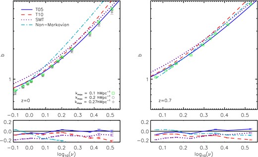
Left: the linear halo mass bias b(logν) measured from the MXXL simulation at z = 0 where |$b = \sqrt{P_{\rm hh}/P_{{\rm m}}}$| using 0.004 < k(h Mpc−1) < 0.1 is shown as green squares. The lines show analytic models from Tinker et al. (2005, blue solid), Tinker et al. (2010, red dashed), Sheth et al. (2001, purple dotted) and the model from Ma et al. (2011, cyan dot–dashed) which includes non-Markovian terms and a stochastic barrier. Right: the halo bias at z = 0.7. All model predictions were generated by scaling the variance of the linear density field by the logarithm of the ratio of the linear growth at z = 0.7 and 0. The Ma et al. (2011) model has been plotted at this redshift (cyan dot–dashed lines) using the best-fitting values to the mxxlb–logν relation. In both cases, the lower panels show the ratio of the model predictions to the mass bias measured from the simulation.
The right-hand side of Fig. 3 compares the bias measured from the mxxl simulation with the models at z = 0.7. In this case, the Tinker et al. (2005) provides a reasonable match to the bias of haloes corresponding to modest peak heights. For rarer peaks, the Sheth et al. (2001) works better at this redshift. Reassuringly, the results presented in this section agree with Gao, Springel & White (2005) over a range of masses. We present several new results in our analysis: we extend these measurements up to log10(ν) = 0.5 at z = 0 and 0.7 allowing us to probe the high-mass end of the b–ν relation; we show several modern analytic fitting formulas for the bias finding that the model of Ma et al. (2011) fit the measurements at the low-mass end; we find that the Tinker et al. (2005) model is successful at fitting the b–ν relation outside the regime where it was calibrated. We are able to measure the bias on very large scales, on which we have demonstrated that the bias is approximately independent of scale; Gao et al. (2005) used the correlation function on modest, quasi-linear scales to estimate the bias.
3.2 Minimizing shot noise
The two main sources of error in a measurement of the power spectrum are cosmic variance, due to a finite number of modes available on large scales with which to determine the variance of the field (see e.g. Bernstein & Cai 2011), and the shot noise due to the discrete sampling of the density field using galaxies or haloes. If we assume Poisson statistics, then the shot noise error equals the inverse of the number density which can be simply subtracted from the overall measurement. Within the halo model where all dark matter lies in collapsed haloes of different masses there should be significant halo exclusion effects for the most massive haloes which will cause discrete sampling effects to deviate from Poisson statistics. Seljak et al. (2009) proposed accounting for this difference using mass-weighting schemes to boost the clustering signal of a halo sample resulting in a shot noise term which is lower than predicted from |$1/\bar{n}$| Poisson statistics. Here, we make use of the cross-correlation power spectra between a high number density halo sample, whose shot noise is negligible, and a high-mass, low number density sample with |$\bar{n} \sim 10^{-4} (h/$| Mpc)3. We focus on a single number density and mass range which will be most affected by shot noise.
H: all haloes with >1012 h−1 M⊙
h: haloes with mass ∈ 3 × 10¹³–1 × 10¹⁴ h−1 M⊙,
In Fig. 4, the z = 0 measured power spectrum with uniform weighting for all haloes with masses M > 1012 h−1 M⊙ and haloes with M = 3 × 10¹³–1 × 10¹⁴ h−1 M⊙ are shown as a solid purple and red line, respectively. The cross spectrum with uniform weighting for these two tracers is shown as a blue solid line. Power spectra using mass weightings for the M ∈ 3 × 10¹³–1 × 10¹⁴ h−1 M⊙ sample are shown as dashed lines. The expected Poisson shot noise for the uniform and mass-weighting schemes are shown as horizontal solid and dashed lines. As can be seen from this plot, the mass-weighting scheme boosts the Poisson shot noise term but also boosts the clustering signal.
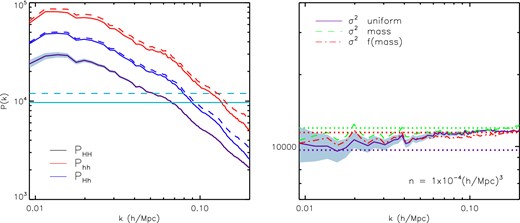
Left: the power spectrum measured at z = 0 with uniform weighting for all haloes with masses M > 1012 M⊙ h−1 and haloes with M ∈ 3 × 10¹³–1 × 10¹⁴ M⊙ h−1 is shown as a solid purple and red line, respectively. The cross spectrum with uniform weighting for these two tracers is shown as a blue solid line. Power spectra using mass weightings for the M ∈ 3 × 10¹³–1 × 10¹⁴ M⊙ h−1 sample are shown as dashed lines. The expected Poisson shot noise for the uniform and mass-weighting schemes are shown as horizontal solid and dashed lines. The grey shaded regions show errors on the uniform weighted P(k) for the halo sample M > 1012 M⊙ h−1. Right: the measured noise and expected Poisson shot noise for different weighting schemes are shown as solid and dotted lines, respectively.
In the right-hand panel of Fig. 4, the measured noise and expected Poisson shot noise for different weighting schemes are shown as solid and dotted lines, respectively. Here, the f(mass-) weighting scheme is the one suggested in Seljak et al. (2009), where |$f(M) = M/(1 + \sqrt{(}M/10^{14}\,h^{-1}\,\mathrm{M}_{\odot })).$| As can be seen from this figure, on large scales, the measured and expected shot noise in the case of uniform weighting agree on large scales (purple solid and dotted lines) but this agreement breaks down as we go to smaller non-linear scales. This may be due to stochasticity on small scales as r differs from unity or the fact that assuming Poisson shot noise overestimates the noise levels for highly biased tracers as found in Seljak et al. (2009). Using either the mass or f(M) weighting schemes, we find a small (a factor of 1.5) reduction in the measured shot noise compared to the expected value from Poisson statistics. These improvements are small compared to the factor of 3 reduction in shot noise which Seljak et al. (2009) found when using the cross-correlation between a halo sample and the dark matter field. Although this approach does not yield such a large reduction in shot noise, the main advantage of this method is that the dark matter density field does not need to be estimated in contrast to the method presented in Seljak et al. (2009). Overall, this method may be further improved using e.g optimal mass-dependent halo weighting as in Hamaus et al. (2010).
4 VELOCITY BIAS
In this section, we examine the statistics of the velocity field measured from the dark matter and halo populations in the mxxl simulation through the auto, Pθθ, and cross, Pδθ, power spectra for the velocity divergence |$\theta \equiv {\nabla } \cdot \boldsymbol {v}/(aH)$|, where a is the scale factor and H is the Hubble rate. These two power spectra are important in many models for redshift-space distortions (see e.g. Scoccimarro 2004; Percival & White 2009; Jennings et al. 2011; Tang, Kayo & Takada 2011; de la Torre & Guzzo 2012). Any bias between the velocity divergence power spectra for a galaxy/halo population and the underlying dark matter would have important implications for cosmological parameters extracted assuming that a tracer population follows the dark matter exactly. To our knowledge, this is the first time that these power spectra have been analysed for different halo populations using simulations.
Measuring the velocity power spectrum accurately from N-body simulations can be difficult as both mass- and volume-weighted approaches can involve significant noise and biases on small scales (Pelupessy, Schaap & van de Weygaert 2003; Scoccimarro 2004; Pueblas & Scoccimarro 2009; Cautun & van de Weygaert 2011; Jennings et al. 2011; Jennings 2012; Hahn, Angulo & Abel 2014). The method suggested by Scoccimarro (2004) allows a mass-weighted velocity field to be constructed but is limited by the fact that it is the momentum field which is calculated on a grid and so the velocity field in empty cells is artificially set to zero (Pueblas & Scoccimarro 2009). Another limitation of this method is that most calculations require the volume-weighted velocity field instead of the mass-weighted field. Using a Delaunay tessellation of a discrete set of points allows the desired volume-weighted velocity field to be constructed accurately on small scales. We use the publicly available dtfe code (Cautun & van de Weygaert 2011) to construct the velocity divergence field for our halo samples directly. This code constructs the Delaunay tessellation from a discrete set of points and interpolates the field values on to a user-defined grid. The density field is interpolated on to the grid using the CIC assignment scheme. The resolution of the mesh means that mass assignment effects are negligible on the scales of interest here.
Given the large number density of particles in the MXXL simulation, it is numerically infeasible to run the dtfe code on the dark matter. Instead, we adopt the mass-weighted method suggested by Scoccimarro (2004) to measure Pθθ and Pδθ for the dark matter particles both at z = 0 and 0.7 using a 10243 grid. Using smaller volume ΛCDM simulations in a box of 1500 h−1 Mpc on a side and 10243 particles from Jennings (2012), we have verified that this mass-weighted method agrees with the dtfe dark matter velocity field up to k ∼ 0.2 h Mpc−1 for Pθθ and k ∼ 0.3 h Mpc−1 for Pδθ. We will restrict our comparison between the velocity statistics for dark matter and haloes to this range where the mass-weighted method has converged. To account for aliasing and shot noise effects on both the halo and dark matter velocity power spectra, we have verified that increasing the size of the grid used (10243) has no effect on the measured power over the range of scales we consider in this work.
Fig. 5 shows the halo velocity power spectra Pθθ (left-hand panel) and Pδθ (right-hand panel) at z = 0 for different mass ranges and number densities given in the legend. For clarity, we only plot the error bars for the 2× 10¹² h−1 M⊙ bin as a grey shaded region. There is a clear difference in the P(k) measured using different halo samples, which increases with increasing mass (decreasing number density) on large scales k > 0.01 h Mpc−1. As shown in Pueblas & Scoccimarro (2009) and Jennings et al. (2011), the velocity power spectrum is very sensitive to resolution and this trend of increasing bias with an increase in the halo mass is actually due to a decrease in the number density of the velocity field tracers. We verify that this is indeed a number density bias by matching number densities for different mass ranges and comparing the measured Pθθ and Pδθ. As can be seen from the black dot–dashed and blue dashed lines in Fig. 5, once we match the number density for these two different mass bins to |$\bar{n} = 1.2 \times 10^{-4}(h/$| Mpc)3, we obtain the same velocity power spectra. We have also verified this for two mass bins which have different bias factors, M = 1.5 × 10¹⁴ h−1 M⊙ (b ∼ 2 at z = 0) and M = 1 × 10¹³ h−1 M⊙ (b ∼ 1 at z = 0), but the same number density |$\bar{n} = 2.8 \times 10^{-5}(h/$| Mpc)3 (green dashed and dot–dashed lines in Fig. 5). Note that the power spectra for all haloes with masses >1012 h−1 M⊙ (purple dot–dashed line) is similar to the sample 1–3 × 10¹² h−1 M⊙ (red dashed line) in this figure, which is why their measured velocity P(k) agree.
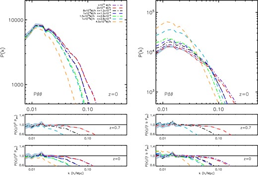
Upper panels: the auto (left) and cross (right) velocity divergence power spectra measured from the mxxl simulation at z = 0 for different mass bins and number densities as shown in the legend. For clarity, only error bars for the 2 × 10¹² h−1 M⊙ bin are plotted (grey shaded region). Lower panels: the z = 0 velocity divergence power spectra normalized by f2Pdark matter and fbPdark matter for the auto and cross power spectra, respectively. Note that the dark blue and grey dashed lines (and green and cyan lines) correspond to different mass ranges but equal number densities. Middle panels: same ratios as the lower panels at z = 0.7.
In the lower four panels in Fig. 5, we show the ratios |$P^{\rm {\rm haloes}}_{\theta \theta }/(f^2 P^{\rm dark matter}_{\delta \delta })$| and |$P^{\rm {\rm haloes}}_{\delta \theta }/(f b P^{\rm dark matter}_{\delta \delta })$| as a function of scale at z = 0 and 0.7 where f ≡ dlnD/dlna is the growth rate (logarithmic derivative of the growth factor, D) and b is the linear bias for each halo sample at that redshift. From the panels, we can see that the velocity P(k) agree with linear theory predictions only on large scales k = 0.004 h Mpc−1 at both redshifts for our halo mass bins 2 × 10¹² h−1 M⊙ (|$\bar{n} = 2.26 \times 10^{-3}(h/$| Mpc)3) and 8× 10¹² h−1 M⊙ (|$\bar{n} = 1.2 \times 10^{-4}(h/$| Mpc)3). Beyond k = 0.004 h Mpc−1, we see a departure from linear theory and a difference of ≈50 per cent between the measured velocity P(k) and linear perturbation theory predictions at k = 0.1 h Mpc−1. For the 1× 10¹³ h−1 M⊙ mass bin, the measured Pθθ and Pδθ only agree with linear theory predictions for k < 0.002 h Mpc−1. We see the largest deviations for the 4.5× 10¹⁴ h−1 M⊙ mass bin, which we were only able to accurately measure at z = 0. It is clear from the ratios in these figures that for small number densities, |$\bar{n} \sim 10^{-6}(h/$| Mpc)3, the sampling bias is extremely large and we do not recover the linear theory prediction for the cross power spectrum on large scales. Note the agreement between the cross spectra and the predictions of linear perturbation theory for these halo velocity divergence power spectra is interesting considering that the linear bias used is defined as an average quantity which takes into account stochasticity b ≡ (Phalo/Pdark matter)1/2 rather than a local linear variable b = δhalo/δdark matter (Matsubara 1999).
In Fig. 6, we compare the measured mxxl matter (black circles) and velocity (black triangles) power spectra for the dark matter and the 2 × 10¹² h−1 M⊙ mass bin velocity P(k) (red squares) with two models which have been calibrated using N-body simulations. We also compare these measured power spectra with the predictions of perturbation theory as in Scoccimarro (2004). The vertical dashed line in each panel indicates the maximum wavenumber where our velocity P(k) have converged. Although the Jennings (2012, green dashed line) and the Hahn et al. (2014, purple dot–dashed line) formulas were calibrated on simulations of different resolutions and cosmologies to the MXXL simulation, and, furthermore, each study used a different method for determining the velocity field, we find very good agreement between both formulas and the measured Pθθ and Pδθ at z = 0 and z = 0.7 for k < 0.15 h Mpc−1. In agreement with Scoccimarro (2004), we find that one-loop perturbation theory (blue dotted line) predictions are accurate for k < 0.1 h Mpc−1. On smaller scales, perturbation theory over (under) predicts the amplitude of the matter (velocity) power spectra for the dark matter.
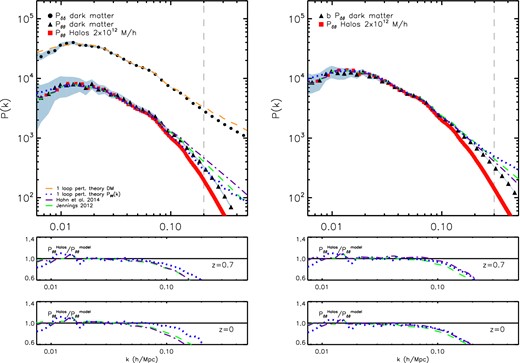
Upper panels: the MXXL matter (black circles) and velocity (black triangles) power spectra for the dark matter at z = 0. The velocity divergence power spectra for the 2 × 10¹² h−1 M⊙ mass bin are plotted as red squares in both panels. The error bars for the dark matter power spectra are plotted as grey shaded regions. The velocity divergence power spectrum predictions from one-loop perturbation theory, Jennings (2012) and Hahn et al. (2014) are shown as blue dotted, green dashed and purple dot–dashed lines, respectively, in all panels. The dark matter P(k) predicted from perturbation theory is shown as an orange dashed line in the upper-left panel only. The vertical dashed line in each panel indicates the maximum wavenumber where our velocity P(k) have converged. Lower panels: the ratio between the power spectra measured for the 2 × 10¹² h−1 M⊙ mass bin halo sample (see labels) and the different model predictions at z = 0. Middle panels: same ratios as shown in the lower panels but for z = 0.7.
As shown in Fig. 5, there is a significant sampling bias between velocity power spectra for mass bins with different number densities. In Fig. 6, it is clear that the dark matter (black circles) and the 2 × 10¹² h−1 M⊙ mass bin (red squares) velocity power spectra only agree up to k < 0.08 h Mpc−1. Even for the largest number density mass bin which we use in this study there is a significant sampling bias between the dark matter and the halo velocity P(k). In order to highlight the discrepancy between the models, which accurately predict the dark matter Pθθ and Pδθ, and the halo velocity divergence power spectra, we plot the ratio of these two power spectra in the lower (z = 0) and middle (z = 0.7) panels in Fig. 6. It is clear from these ratio plots that all models for the dark matter velocity statistics are biased by approximately 20 per cent for Pθθ and approximately 10 per cent for Pδθ at k = 0.1 h Mpc−1 compared to the halo velocity divergence P(k). This discrepancy is significant and will have an impact on cosmological parameter inference from e.g. redshift-space clustering measurements where redshift-space distortions models assume zero velocity bias. The question of how to correct for this sampling bias in both power spectra as a function of scale is beyond the scope of this work and is left for future study. Note while writing up this paper we became aware of two recent studies by Baldauf et al. (2014) and Zhang et al. (2014) who have also reported that there should be a bias in the velocity power spectra. Zhang et al. (2014) report that the velocity divergence auto power spectra for |$\bar{n} \sim 10^{-3}(h/$| Mpc)3 tracers should be affected by approximately 10 per cent at k = 0.1 h Mpc−1, in agreement with our findings.
5 CONCLUSIONS AND SUMMARY
We have tested various models for the linear halo mass bias using measurements of the ratio of the halo auto power spectra from the MXXL simulation at redshifts z = 0 and 0.7 for different mass bins in the range 2 × 10¹²–1.5 × 10¹⁵ h−1 M⊙. In agreement with the work of Angulo et al. (2008) and Okumura & Jing (2011), we find that the assumption of a linear bias is only valid on scales k < 0.2 h Mpc−1 for masses <2 × 10¹³ h−1 M⊙ and k < 0.1 h Mpc−1 for masses >6 × 10¹³ h−1 M⊙ at z = 0. At a higher redshift of z = 0.7, this bias is remarkably scale independent for all masses at k < 0.1 h Mpc−1 although the scale dependence is more pronounced on quasi-linear scales compared to redshift zero. When fitting for a linear scale-independent bias, we find a gradual decline in the best-fitting value with increasing kmax instead of a sharp jump which would have suggested the onset of a pronounced scale-dependent bias and hence a clearly motivated value for kmax.
When plotted as a function of peak height, we find that the bias–logν relation is well fitted at z = 0 by the model of Tinker et al. (2005) except for low-mass haloes <7 × 10¹² h−1 M⊙ whose bias is overpredicted by the model. We find that the non-Markovian and diffusive barrier model of Maggiore & Riotto (2010) is a better fit to the linear bias of these low-mass haloes. At redshift z = 0.7, we find that the linear bias of MXXL FOF haloes more massive than 1013 h−1 M⊙ is better fitted by the ellipsoidal collapse model of Sheth et al. (2001) which is accurate to ∼5 per cent when fitting over the range 0.004–0.1 h Mpc−1. We find that the model of Tinker et al. (2010), which was calibrated on SO haloes, overestimates the FOF halo bias from the MXXL simulation at both redshifts by approximately 10–20 per cent over the range of masses we consider.
We have investigated different weighting schemes applied to the dark matter halo power spectra clustering measurements in order to reduce the shot noise for a high-mass (low number density) sample. We have modified the approach of Seljak et al. (2009) who made use of the cross-correlation power spectra between the haloes and dark matter to measure the actual shot noise (assuming deterministic biasing on large scales). Seljak et al. (2009) found that mass weighting could lower the shot noise compared with Poisson statistics by a factor of 3 for a |$\bar{n} \sim 10^{-4} (h/$| Mpc)3 sample. Here, we make use of the cross-correlation power spectra between a large number density halo sample, whose shot noise is negligible, and a high-mass (low number density) sample with |$\bar{n} \sim 10^{-4} (h/$| Mpc)3. We find that mass weighting is able to reduce the shot noise of the measured power spectra by at most a factor of 1.5 compared to the Poisson estimate. Although this approach does not yield such a large reduction in shot noise, the main advantage of this method is that the dark matter density field does not need to be estimated in contrast to the method presented in Seljak et al. (2009).
We have measured the velocity divergence auto, Pθθ, and cross, Pδθ, power spectra for a range of halo masses from the MXXL simulation at redshifts z = 0 and 0.7. This is the first time that these velocity statistics have been presented and compared with the dark matter velocity power spectra from a simulation. The high mass and force resolution of the MXXL simulation allows us to reconstruct the velocity power spectra for haloes masses 1012–6 × 10¹⁴ h−1 M⊙ up to k = 0.1 h Mpc−1 and the dark matter velocity power spectra up to k = 0.2 h Mpc−1 (k = 0.3 h Mpc−1) for Pθθ (Pδθ) at z = 0. We find that there is a significant sampling bias in both velocity divergence power spectra at z = 0 and 0.7 which decreases the measured power compared to the dark matter velocity P(k) by approximately 20 per cent at k = 0.1 h Mpc−1 for a |$\bar{n} = 2 \times 10^{-3} (h/$|Mpc)3 sample. This sampling bias increases to ∼40 per cent for a |$\bar{n} = 1.2 \times 10^{-4} (h/$|Mpc)3 sample at k = 0.07 h Mpc−1. If neglected, this bias would have a significant impact on cosmological parameter constraints extracted from redshift-space clustering measurements which use fitting formula or perturbation theory predictions for the dark matter velocity divergence power spectra.
Current and future large galaxy redshift surveys will map the three-dimensional galaxy distribution to a high precision. There is an major ongoing effort to advance the models for the clustering signal in redshift space where the observed redshift is composed of both the peculiar velocities of galaxies and a cosmological redshift from the Hubble expansion. It is well known that any scale-dependent bias between haloes and the dark matter would be a key systematic affecting cosmological parameter constraints. In this paper, we have used one of the highest resolution simulations to date to test currently used models for the linear bias beyond the mass limits where they were calibrated. We also draw attention to another potentially serious systematic due to a sampling bias in the halo velocity power spectra which would affect the comparison between observations and any redshift-space distortion model which assumes dark matter velocity statistics. We leave further analysis and modelling of this bias to future research.
The authors are grateful to Raul Angulo and Volker Springel for comments on this paper and for allowing the MXXL outputs to be used in this study. The MXXL simulation was carried out on Juropa at the Juelich Supercomputer Centre in Germany. EJ acknowledges the support of a grant from the Simons Foundation, award number 184549. This work was supported in part by the Kavli Institute for Cosmological Physics at the University of Chicago through grants NSF PHY-0114422 and NSF PHY-0551142 and an endowment from the Kavli Foundation and its founder Fred Kavli. This work was supported by the Science and Technology Facilities Council (grant number ST/L00075X/1). This work used the DiRAC Data Centric system at Durham University, operated by the Institute for Computational Cosmology on behalf of the STFC DiRAC HPC Facility (www.dirac.ac.uk). This equipment was funded by BIS National E-infrastructure capital grant ST/K00042X/1, STFC capital grant ST/H008519/1, and STFC DiRAC Operations grant ST/K003267/1 and Durham University. DiRAC is part of the National E-Infrastructure. We are grateful for the support of the University of Chicago Research Computing Center for assistance with the calculations carried out in this work.
