


Abstract
We propose a new fast method for estimation of the impact probability of near-Earth objects (NEOs), based on the assumption that the errors in coordinates and velocities have a normal distribution at all times. In this method, a unique coordinate system associated with the nominal orbit of an asteroid is used. One of the coordinates of this system is the mean anomaly in the osculating orbit of an asteroid. This system allows one to take into account the distribution of virtual asteroids mainly along the nominal asteroid orbit. The probability is calculated as a six-dimensional integral of the probability density functions of coordinates and velocity errors. This method has a limitation on usage due to this assumption. Close approaches to massive bodies can break the normal distribution of virtual asteroids and disturb the impact probability value. The impact probabilities for eight asteroids have been calculated by the proposed method. A comparison of these values with probabilities obtained by the Monte Carlo method shows good agreement for seven of them. For 2007 VK184, which has three close approaches to major planets, the impact probability obtained by the new method differs by about five times, but the proposed method takes several orders of magnitude fewer computation time than the Monte Carlo one. Also, we have demonstrated the advantage of using a curvilinear coordinate system in comparison with a Cartesian one.
1 INTRODUCTION
The problem of estimating the impact probability of an asteroid with the Earth at time t and times in its vicinity can be separated into two subproblems. The first one consists of determining the nominal orbit, which is described by six orbital parameters, and finding the distribution function of their errors. The area of parameter errors can be described by a ‘cloud’ of virtual asteroids (VAs). This cloud surrounds the position of an asteroid in the nominal orbit and the cloud size and density are determined by a function of the distribution of parameter errors. The second problem is to determine the positions of VAs at time t and to estimate their impact possibilities with the Earth.
A more efficient method is the method called line-of-variation sampling (Milani et al. 2002). In this method, instead of a six-dimensional cloud of VAs, we consider a one-dimensional region that is hopefully representative of the entire six-dimensional one. For this purpose, we can use the line of variations (LOV), which is the line of weakness of the orbit determination solution. This line is defined by the eigendirection associated with the largest eigenvalue of the correlation matrix. In order to find this eigendirection, the singular decomposition of the correlation matrix can be used. Choosing VAs along the LOV, we determine a region of VAs that will collide with the Earth. Even though interpolation along the LOV is generally more efficient than the Monte Carlo method, we cannot be confident that the LOV approach will detect all potential collisions (Milani et al. 2002). Also, it requires one to perform simulations too, but not as many as in the Monte Carlo method. In Milani et al. (2005a), one can see the theory for generating the LOV and Milani et al. (2005b) include techniques for nonlinear impact hazard assessment.
Nowadays, a great number of near-Earth objects (NEOs) are discovered and the amount of asteroids discovered per month increases. We need to be able to estimate their impact probabilities quickly.
In this work, we propose a new high-speed method based on the assumption that the parameter errors of an asteroid's orbit have a normal distribution at all times. Methods based on this assumption are generally called linear methods of impact probability estimation. This assumption leads to limitations in using these methods. Gravitational perturbations from massive bodies, which significantly change the orbit of an object, can break the normal distribution of parameter errors of an asteroid's orbit and hence distort the impact probability value. Also, since the distribution of VAs is mainly along the nominal orbit (if the possible collision time is far from the last observation), the normal distribution law of VAs in Cartesian coordinates does not imply a real one. Consequently, linear methods, which use a Cartesian coordinate system (e.g. the target-plane method: Milani et al. 2002), have an added limitation in their usage. In this work, we try to eliminate the last limitation. In order to do this, we introduce a special curvilinear coordinate system that allows us to take into account the distribution of VAs mainly along the nominal orbit at time t, even if t is far from the last observation. Also, a comparison between using Cartesian and introduced coordinate systems is given in this work.
2 THE GENERAL IDEA
It is convenient to use coordinates and velocities as orbital parameters to define Θ. In this case, in the space of velocities, Θ is (−∞, +∞) × (−∞, +∞) × (−∞, +∞). Consequently, the six-dimensional integral can be integrated analytically over the velocity components. Let (x4, x5, x6) denote the velocity components. Consider integrating (1) over the component x6.
3 NEW COORDINATE SYSTEM
If the time at which it is necessary to estimate the probability of collision differs by some revolution periods of a small body around the Sun from the time of the last observation, the area of possible positions of VAs is noticeably stretched along the nominal orbit, due to distinctions in the mean motions of VAs. Eventually the difference in the travelled path of VAs can reach an entire revolution, although variations of their positions in the plane perpendicular to the orbit can remain small. It is difficult to take this fact into account using a normal distribution in Cartesian coordinates.
We propose using a curvilinear frame (ξ, η, M) related to the nominal orbit. To construct this system, we do the following. First of all, we fix the osculating ellipse of a small body at time t (i.e. the five parameters of the osculating ellipse). The mean anomaly M in the osculating orbit is one of the coordinates of this system. The origin of the linear coordinates ξ, η is the point on the ellipse corresponding to M.
The axis η lies in the plane of the fixed ellipse. Let A be a point, the ξ, η, M coordinates of which are determined, and B be the projection of point A on to the plane of the fixed ellipse. The η-axis contains point B. This system is required to be orthogonal (i.e. the vectors |$\boldsymbol {e_{\xi }}, \boldsymbol {e_{\eta }}, \boldsymbol {e_M}$| must be mutually orthogonal vectors). This system is schematically illustrated in Fig. 1.
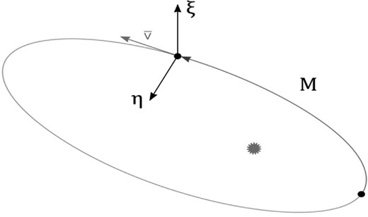
The (ξ, η, M) coordinate system.
Note that at M = 0 and M = π the left-hand side of the above equation has different signs, hence in both regions [0, π) and [π, 2π) there is at least one root. We choose the root (M) that corresponds to the closest point to (x0, y0).
4 CALCULATING AN IMPACT PROBABILITY
The normal matrix in Cartesian coordinates and velocities at time t is defined as |${{\bf N}_{xyz}} = (\mathbf {\boldsymbol\Phi }^{\rm T})^{-1} \cdot {{\bf N}_{xyz}^0} \cdot \mathbf {\boldsymbol\Phi }^{-1}$|. The osculating ellipse is fixed. The asteroid's coordinates and velocities in the introduced coordinate system |$\xi , \eta , M, \dot{\xi },\dot{\eta },\dot{M}$| are computed (|$\xi =\eta =\dot{\xi }=\dot{\eta }=0$|, since the asteroid is in the osculating ellipse).
Now we have to define the region Θ in the introduced coordinate system. In order to do this, we modify the introduced system so that Θ has a sphere-like shape. Let the coordinates of the Earth's centre in this system be (ξt, ηt, Mt). Then the projection of Θ on to the coordinate M is the interval |$[-\frac{R_\oplus}{V}\dot{M}+M_t,\, \frac{R_\oplus }{V}\dot{M}+M_t]$|, where R⊕ is the Earth's radius and V is the magnitude of the heliocentric velocity of the asteroid at time t.
Consider the coordinate system (ξ, η, M/d), where |$d = {\dot{M}}/{V}$|. In this frame, the projection Θ on to the (ξ, η) plane is a circle with radius R⊕ and the projection Θ on to the coordinate M/d is an interval with semi-length also R⊕. Since the Earth's radius R⊕ ≪ 1au, Θ can be considered as a full sphere in coordinates (ξ, η, M/d). This is a good approximation to estimate an impact probability. In order to find the normal matrix |${\bf N}$|ξη(M/d) in the coordinates (ξ, η, M/d), we need to multiply the elements of the matrix |${{\bf N}_{\xi \eta M}^{\prime }}$| in the third column and the elements in the third row by d (in this case the element in the third column and third row is multiplied by d2).
Using singular decomposition allows us to decrease the computation time of the integral by several orders of magnitude.
5 RESULTS
To verify this method, we considered impact probabilities for eight asteroids. We chose these asteroids randomly from the website of the Jet Propulsion Laboratory, NASA,1 but ensuring impact probabilities more than 10−7. Their orbits were calculated by a method based on an exhaustive search for orbital planes (Bondarenko, Vavilov & Medvedev 2014). The normal matrix at the initial epoch was computed by a differential method. In Table 1, the characteristics of asteroid orbits are represented. The selected asteroids have different values of orbital inclinations 0.9 < i < 25.1 and a wide range of eccentricities 0.16 < e < 0.74.
Characteristics of asteroid orbits.
| Object | a (au) | e | i (°) | σ (′′) | ΔT (d) | k |
|---|---|---|---|---|---|---|
| 2006 QV89 | 1.20 | 0.23 | 1.1 | 0.44 | 10.83 | 68 |
| 2007 VK184 | 1.73 | 0.57 | 1.2 | 0.39 | 60.01 | 102 |
| 2008 CK70 | 1.11 | 0.46 | 6.0 | 0.44 | 4.66 | 77 |
| 2009 JF1 | 1.87 | 0.74 | 6.0 | 0.55 | 1.23 | 25 |
| 2008 JL3 | 2.16 | 0.54 | 0.9 | 0.40 | 4.10 | 31 |
| 2005 BS1 | 1.97 | 0.57 | 2.6 | 0.57 | 3.13 | 25 |
| 2005 QK76 | 1.40 | 0.52 | 22.9 | 0.65 | 1.68 | 14 |
| 2007 KO4 | 1.10 | 0.16 | 25.1 | 0.49 | 3.00 | 14 |
Notes: ‘Object’ is the asteroid designation, a the semi-major axis, e eccentricity, i orbital inclination, σ the root-mean-square error of observations, k the number of observations and ΔT the arc of observations.
The impact probabilities for these eight asteroids were calculated by the proposed method in the introduced coordinate system (ξ, η, M). Also, we calculated them using the scheme described above in a Cartesian coordinate system. To check the values obtained, the probabilities were also computed by the Monte Carlo method. The absolute error of probability calculated by the Monte Carlo method is estimated according to |$\sigma _{\rm MC} = ({\sqrt{P_{\rm MC}(1-P_{\rm MC})}})/{\sqrt{m}}$|, where m is the number of realizations, PMC the probability and relative error δMC = σMC/PMC. Results of calculations are given in Table 2, where ‘object’ is the asteroid designation, PξηM and Pxyz are the probabilities calculated by the proposed method in the coordinate system (ξ, η, M) and in a Cartesian coordinate system, respectively, and t is the time at which the impact probability calculated by this method reaches its maximum value. To find t, we calculated impact probabilities at different times in the vicinity of some initial approximation of t. As initial approximation, we took the time when the distance between the Earth and the nominal asteroid orbit is minimum. We calculate this time using the program of Baluyev for determining Minimum Orbital Intersection Distance (Kholshevnikov & Vasiliev 1999; Baluyev & Kholshevnikov 2005).
Comparison of different methods of estimation of impact probabilities.
| Object | t (d) | Pxyz | PξηM | PMC | 3δMC (per cent) | ΔPxyz (per cent) | ΔPξηM (per cent) | COP |
|---|---|---|---|---|---|---|---|---|
| 2006 QV89 | 2019 Sep 09.38 | 2.5 × 10⁻³ | 2.2 × 10⁻³ | 1.8 × 10⁻³ | 6 | 39 | 23 | 4.7 × 10⁻³ |
| 2007 VK184 | 2048 Jun 03.09 | 2.9 × 10⁻⁵ | 3.0 × 10⁻⁵ | 6.2 × 10⁻⁶ | 32 | 364 | 387 | 2.8 × 10⁻³ |
| 2008 CK70 | 2030 Feb 14.67 | 6.7 × 10⁻⁴ | 6.4 × 10⁻⁴ | 6.4 × 10⁻⁴ | 15 | 4 | 0 | 6.7 × 10⁻⁴ |
| 2009 JF1 | 2022 May 06.34 | 6.7 × 10⁻⁴ | 6.6 × 10⁻⁴ | 7.4 × 10⁻⁴ | 16 | −10 | −12 | 6.6 × 10⁻⁴ |
| 2008 JL3 | 2027 May 01.41 | 4.7 × 10⁻⁴ | 4.7 × 10⁻⁴ | 3.0 × 10⁻⁴ | 15 | 59 | 58 | 4.7 × 10⁻⁴ |
| 2005 BS1 | 2016 Jan 14.44 | 0 | 1.5 × 10⁻⁴ | 1.4 × 10⁻⁴ | 16 | −100 | 2 | 1.6 × 10⁻⁴ |
| 2005 QK76 | 2030 Feb 26.32 | 0 | 3.8 × 10⁻⁵ | 4.3 × 10⁻⁵ | 20 | −100 | −12 | 4.1 × 10⁻⁵ |
| 2007 KO4 | 2015 Nov 23.20 | 0 | 4.0 × 10⁻⁷ | 7.3 × 10⁻⁷ | 54 | −100 | −46 | 2.5 × 10⁻⁶ |
For illustration of the accuracy of the methods, in Table 2 we present ΔPxyz and ΔPξηM. These values are the relative distinction of Pxyz and PξηM from PMC, respectively, and are given by ΔP = (P − PMC)/PMC. If value ΔP > 0, then the impact probability obtained by the proposed method is ΔP per cent higher than the one calculated by the Monte Carlo method; otherwise, if ΔP < 0, the impact probability obtained by the proposed method is lower.
We also presented in Table 2 a maximum impact probability, which was introduced by Chesley (2006). We propose to call it the Collisional Orbit Probability (COP). This is the impact probability at time t that the asteroid would have if it passed through the centre of the Earth at time t (and has the same distribution of VAs). This value indicates the size of the dispersion ellipsoid. The larger this value, the smaller the size of the dispersion ellipsoid of VAs at time t. The value of COP depends on the method used to calculate it and has the same limitations. If this value is calculated using this method, the coordinates of the Earth's centre are taken to be zero (ξt = ηt = Mt = 0).
The table shows that the probabilities PξηM are close to those obtained by the Monte Carlo method, but the proposed method requires much less time for calculation (e.g. four million times less for 2007 KO4: it takes about 2 s using an Intel Core i7-2600 3.40-GHz processor). Also, the relative errors of the Monte Carlo method (3δMC) are small, i.e. the values PMC are accurate enough. The exception is asteroid 2007 VK184. The PξηM value for this object is 384 per cent higher than PMC (about five times). This is likely due to close approaches to the Earth (in 2014, distance r = 0.177 au), Venus (in 2030, r = 0.064 au) and Mars (in 2036, r = 0.066 au). However, the COP value for this asteroid obtained by the Monte Carlo method equals (2.76 ± 0.13) × 10−3, which coincides with the one obtained by the proposed method (2.77 × 10⁻³). Therefore the value of COP seems to be more stable.
The impact probabilities of the three asteroids obtained in Cartesian coordinates equal zero (ΔPxyz = −100 per cent). Note that for these asteroids the values of COP are the smallest, i.e. the dispersion ellipsoids of VAs are the largest. Since the extension of the area of VA distribution is mainly along the nominal orbit of an asteroid, then the greater this area the more the VA distribution in Cartesian coordinates differs from the real distribution of VAs. For five asteroids, the value PξηM is close to COP, indicating that the nominal orbit of the asteroid does not differ strongly from one that leads to collision.
In Fig. 2, the impact probability of the asteroid 2008 JL3 as a function of time (in the vicinity of May 1) is represented. The probability grows immediately from 10−35 to the maximum value 4.7 × 10⁻⁴. The region where the probability reaches its maximum value is about 0.06 d (≈90 min). The small size of this time region is a consequence of small errors of ξ and η and a large error of the mean anomaly. Due to this, the maximum value of probability is close to the cumulative one. The behaviour of the impact probability is similar for all asteroids considered.
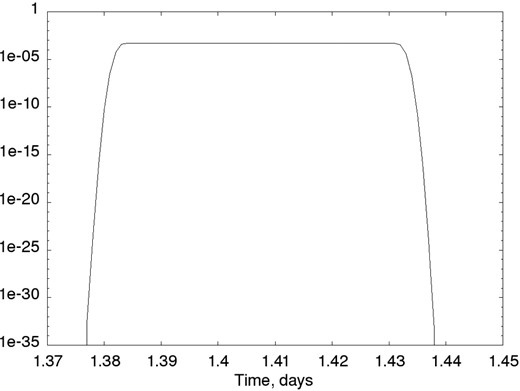
Impact probability of 2008 JL3 on 2027 May 1.
6 CONCLUSION
A high-speed method for estimation of the impact probability of asteroids with the Earth has been developed. This method is based on the assumption that errors in the coordinates and velocities of an asteroid have a normal distribution at all times. The important advantage of this method is using the unique coordinate system related to the nominal orbit of an asteroid. This system allows one to take into account the distribution of VAs mainly along the nominal orbit. The mean anomaly M in the osculating orbit of the asteroid is one of the coordinates of the system introduced; the other two coordinates ξ, η are linear ones and their origin lies in the osculating orbit. The probability is calculated as a six-dimensional integral of VA distribution function. Also, we proposed a technique that allows us to decrease by several orders of magnitude the time of this integral's computation in the introduced coordinate system.
This method can give inaccurate values of the impact probability in cases when there are close approaches to massive bodies before the potential collision, which can break the normal distribution of asteroid parameter errors. However, it works well enough and quickly if close approaches either are absent or do not have a noticeable effect on the result. It should be emphasized that newly discovered objects generally have a short observation arc and few observations; hence generally they have large errors in their orbit parameters. In this case, at the time of close approach we can estimate the impact probability using the proposed method, yet after this close approach the orbit parameter errors become much larger and therefore the impact probability becomes much smaller, so it can make no sense to calculate it after close approach.
The impact probabilities for eight asteroids have been calculated by the proposed method. Comparison of these values with values obtained by the Monte Carlo method for seven of them shows good agreement. The impact probability for asteroid 2007 VK184 obtained by the proposed method is about five times higher than the one obtained by the Monte Carlo method. This is likely due to close approaches with the Earth, Mars and Venus before the time of potential collision. Also in this work, we illustrated the advantage of using the new system instead of a Cartesian one. To estimate the size of the dispersion ellipsoid of VAs we used an indicator COP (Collisional Orbit Probability), which equals the impact probability at time t that the asteroid would have if it passed through the centre of the Earth at time t. The value of COP depends on the method used to calculate it and has the same limitations. Nevertheless, the value of COP seems to be more stable than the impact probability value. We found a dependence between this indicator COP and those asteroids for which the values of impact probabilities obtained in a Cartesian coordinate system are unsatisfactory.
We are very grateful to S. R. Chelsey for useful advices and helpful comments. This work is supported by the Institute of Applied Astronomy of Russian Academy of Science.
