


Abstract
Ultrafast outflows (UFOs) are seen in many AGN, giving a possible mode for AGN feedback on to the host galaxy. However, the mechanism(s) for the launch and acceleration of these outflows are currently unknown, with UV line driving apparently strongly disfavoured as the material along the line of sight is so highly ionized that it has no UV transitions. We revisit this issue using the Suzaku X-ray data from PDS 456, an AGN with the most powerful UFO seen in the local Universe. We explore conditions in the wind by developing a new 3D Monte Carlo code for radiation transport. The code only handles highly ionized ions, but the data show the ionization state of the wind is high enough that this is appropriate, and this restriction makes it fast enough to explore parameter space. We reproduce the results of earlier work, confirming that the mass-loss rate in the wind is around 30 per cent of the inferred inflow rate through the outer disc. We show for the first time that UV line driving is likely to be a major contribution to the wind acceleration. The mass-loss rate in the wind matches that predicted from a purely line driven system, and this UV absorption can take place out of the line of sight. Continuum driving should also play a role as the source is close to Eddington. This predicts that the most extreme outflows will be produced from the highest mass accretion rate flows on to high-mass black holes, as observed.
1 INTRODUCTION
AGN-driven winds are potentially the most effective way of transporting energy and momentum from the nuclear scales to the host galaxy, quenching star formation in the bulge by sweeping away the gas reservoir. This feedback process can quantitatively reproduce the M–σ relation (e.g. King 2010).
We see clear observational evidence of winds in AGN via absorption lines. In the UV and X-ray bands, we observe narrow absorption lines outflowing with moderate velocity of hundreds to few thousand km s−1. This warm absorber is detected in 50 per cent of AGN (Blustin et al. 2005; Piconcelli et al. 2005; McKernan, Yaqoob & Reynolds 2007), and may have its origin in a swept-up ISM or thermally driven wind from the molecular torus (Blustin et al. 2005). However, this carries only a small fraction of the kinetic energy, as the amount of material and outflow velocity are both quite small (e.g. Blustin et al. 2005).
Instead, there are two much higher velocity systems which potentially have much greater impact on the host galaxy. In the UV band, broad absorption lines are seen in ∼30 per cent of AGN, and may be present but outside the line of sight in most AGN (Elvis 2000; Ganguly & Brotherton 2008). These absorbers can be outflowing as fast as ∼0.2c, so carry considerable kinetic energy, and probably arise in a UV-line driven wind from the accretion disc (e.g. Proga & Kallman 2004).
However, the most powerful outflows appear to be so highly ionized that the only bound transitions left are for hydrogen- and helium-like iron. Such winds can only be detected at X-ray energies, and a few AGN have substantial columns of material outflowing at speeds of up to ∼0.3c (Tombesi et al. 2010; Gofford et al. 2013), and in a handful of higher redshift AGN at up to 0.7c (Chartas et al. 2002; Lanzuisi et al. 2012). These high velocities point to an origin very close to the supermassive black hole, but the launching and acceleration mechanism remain unclear. Possibilities include radiation-driven winds as the source approaches/exceeds Eddington (King 2010) and/or magnetic driving (e.g. Blandford & Payne 1982), but UV line driving is generally not thought to be important as the high-ionization state of the material means it has negligible UV opacity (Tombesi et al. 2013).
The lack of insight into the wind acceleration mechanism means that even the best wind models are somewhat ad hoc, and impose a geometry and velocity structure on the wind. The wind is probably not spherical (Elvis 2000), so the radiative transfer cannot be modelled analytically via the Sobolov approximation. Instead, the best current codes do full Monte Carlo radiative transfer through the wind material, solving also for the ionization balance at each point in the wind (Sim et al. 2008, 2010a,b). However, such a detailed ionization calculation is slow, so exploring parameter space is difficult.
Here, we develop a new Monte Carlo code, using only the H- and He-like ion stages (see also Sim et al. 2008, 2010a) so that it is fast. We use this to fit to PDS 456 (z = 0.184), one of the most luminous objects in the local Universe (z < 0.3). This is intrinsically of similar luminosity in the optical than 3C 273, though it is heavily absorbed by E(B−V) = 0.48 as it lies close to the plane of our Galaxy (Simpson et al. 1999). This also hosts the most powerful outflow known in the local Universe (Reeves, O'Brien & Ward 2003; Reeves et al. 2009; Tombesi et al. 2010; Gofford et al. 2013), lending support to the radiation-driven wind models since the luminosity is close to Eddington for its ∼2 × 10⁹ M⊙ black hole (Reeves et al. 2009).
We use Suzaku data of PDS 456 (Reeves et al. 2009, 2014; Gofford et al. 2014) for this work because it has a low and stable background and the best spectral resolution with a relatively large collecting area in the Fe K band. Thanks to these capabilities, Suzaku is best suited to study the highly blue-shifted Fe K absorption lines.
The wind in PDS 456 has previously been studied using the Sim et al. (2010a) code by Reeves et al. (2014). We obtain similar results for similar parameters, demonstrating that the new code is reliable, but we are also able to use our fast code to explore a wide range of parameter space, and show how the observed properties of the wind change with each physical parameter. We reproduce all the Suzaku observations of PDS 456, and we can explain the time variability of the wind spectrum in the single modelling framework. We speculate that the wind is launched by a combination of UV-line driving and radiation pressure, but that the UV line driving region is close to the disc, out of the line of sight.
Below, we assume a standard cosmology with H0 = 71 km s−1 Mpc−1, Ωm = 0.27 and |$\Omega _\Lambda =0.73$|, so that the redshift of the target z = 0.184 corresponds to the luminosity distance of dL = 884 Mpc.
2 OBSERVATIONAL DATA: PDS 456
PDS 456 has been observed between 2007 and 2013 with Suzaku (Mitsuda et al. 2007), for a total of five epochs as summarized in Table 1. Among these observations we choose the 2007 data, as this has strong wind absorption lines from H- and He-like iron. It also has a steep spectrum with very little absorption from lower ionization species as required by our code (see Reeves et al. 2009, 2014).
Suzaku observations of PDS 456.
| Obs ID | Start date | Net exposure (ks) |
|---|---|---|
| 701056010 | 2007-02-24 17:58:04 | 190.6 |
| 705041010 | 2011-03-16 15:00:40 | 125.5 |
| 707035010 | 2013-02-21 21:22:40 | 182.3 |
| 707035020 | 2013-03-03 19:43:06 | 164.8 |
| 707035030 | 2013-03-08 12:00:13 | 108.3 |
| Obs ID | Start date | Net exposure (ks) |
|---|---|---|
| 701056010 | 2007-02-24 17:58:04 | 190.6 |
| 705041010 | 2011-03-16 15:00:40 | 125.5 |
| 707035010 | 2013-02-21 21:22:40 | 182.3 |
| 707035020 | 2013-03-03 19:43:06 | 164.8 |
| 707035030 | 2013-03-08 12:00:13 | 108.3 |
We processed and screened X-ray imaging spectrometer (XIS) data by running aepipeline and applied default data screening and cleaning criteria: grade 0, 2, 3, 4 and 6 events were used, while hot and flickering pixels were removed, data were excluded within 436 s of passage through the South Atlantic Anomaly, and within an Earth elevation angle (ELV) < 5° and Earth day-time elevation angles (DYE_ELV) < 20°. The total net exposure time is 190.6 ks. Spectra were extracted from circular regions of 2.9 arcmin diameter, while background spectra were extracted from annular region from 7.0 to 15.0 arcmin diameter. We generated the corresponding response matrix and auxiliary response files by utilizing xisrmfgen and xissimarfgen. The spectra and response files for the two front-illuminated XIS 0 and XIS 3 chips were combined using the ftool addascaspec. The XIS spectra were subsequently grouped to half width at half maximum (HWHM) XIS resolution of ∼0.075 keV at 5.9 keV and ∼0.020 keV at 0.65 keV, and then grouped to obtain a minimum 40 counts in each bin.
Since the main interest of this paper is emission and absorption feature from the H- and He-like iron, we ignore the spectrum below 2 keV (observed frame) to exclude the soft excess. We assume that the 2–10 keV continuum can be modelled by a power law over this restricted energy band, with column density fixed to the Galactic value of 2 × 1021 cm−2. In the remainder of this section, we use phenomenological models for the absorption and emission at iron to connect to previous studies. We then use these to estimate the input parameters for Monte Carlo simulations of the wind (Section 3.2). We show all spectra in the rest frame of PDS 456.
2.1 Gaussian absorption and emission
We fit two negative Gaussian lines to characterize the absorption, plus a single positive Gaussian line to characterize the emission atop a power-law continuum. The equivalent width of the absorption lines is |$0.110^{+0.035}_{-0.028}$| (He-like) and |$0.094_{-0.035}^{+0.025}$| keV (H-like). We confirm the results of Reeves et al. (2009) that the He-like and H-like absorption features have slightly but significantly different blueshift, at vout = 0.295 ± 0.005c (He-like) and 0.310 ± 0.007c (H-like). The two absorption lines are constrained to have the same intrinsic width, which is marginally resolved (σ = 0.048(<0.096) keV). By constrast, the emission line is extremely broad, with |$\sigma =1.3_{-0.6}^{+1.5}$| keV and equivalent width |$0.35_{-0.28}^{+0.28}$| keV. The power-law continuum is quite steep at |$\Gamma =2.34_{-0.05}^{+0.10}$|, and this is a good fit overall, with χ2 = 99.33/98. All parameters are listed in Table 2, and all spectra and models are shown in Fig. 1.
Spectral parameters for the 2007 spectrum.
| Model | Fit | Value |
|---|---|---|
| component | parameter | (90 per cent error) |
| Power law | Gaussian absorption and emission | |
| Γ | |$2.34^{+0.10}_{-0.05}$| | |
| |$F_\mathrm{2{\rm -}10\, keV}$| (10−12 erg s−1 cm−2) | |$3.77^{+0.07}_{-0.22}$| | |
| |$L_\mathrm{2{\rm -}10\, keV}$| (1044 erg s−1) | |$3.52^{+0.07}_{-0.21}$| | |
| Fe xxv | vout | |$0.295^{+0.005}_{+0.005}c$| |
| (6.6975 keV) | σ (keV) | 0.048( < 0.096) |
| EW (keV) | |$0.110^{+0.035}_{-0.028}$| | |
| Fe xxvi | vout | |$0.310^{+0.007}_{-0.007}c$| |
| (6.9661 keV) | σ | Tied to Fe xxv |
| EW (keV) | |$0.094^{+0.025}_{-0.035}$| | |
| Emission | LineE (keV) | |$6.74^{+0.47}_{-1.32}$| |
| σ (keV) | |$1.27^{+1.48}_{-0.59}$| | |
| EW (keV) | |$0.35_{-0.28}^{+0.28}$| | |
| Fit statistics | χ2/dof | 93.33/98 |
| Null probability | 0.61 | |
| χ2/dof for 6.5–10.0 keV | 13.90/20 | |
| kabs + Gaussian emission | ||
| Power law | Γ | |$2.32_{-0.05}^{+0.06}$| |
| |$F_\mathrm{2{\rm -}10\, keV}$| (10−12 erg s−1 cm−2) | |$3.78_{-0.12}^{+0.11}$| | |
| |$L_\mathrm{2{\rm -}10\, keV}$| (1044 erg s−1) | |$3.53_{-0.11}^{+0.10}$| | |
| Fe xxv | vout | |$0.294_{-0.004}^{+0.004}c$| |
| kT (keV) | 474( < 10 484) | |
| Natom (1018) | |$3.7_{-2.1}^{+18.9}$| | |
| EW (keV) | 0.122 | |
| Fe xxvi | vout | |$0.310_{-0.006}^{+0.007}c$| |
| kT (keV) | Tied to Fe xxv | |
| Natom (1018) | |$3.0_{-1.7}^{+8.1}$| | |
| EW (keV) | 0.097 | |
| Emission | LineE (keV) | |$6.8_{-0.6}^{+0.4}$| |
| σ (keV) | |$1.1_{-0.9}^{+0.9}$| | |
| EW (keV) | |$0.271_{-0.182}^{+0.199}$| | |
| Fit statistics | χ2/dof | 91.74/98 |
| Null probability | 0.66 | |
| χ2/dof for 6.5–10.0 keV | 13.09/20 | |
| pcygx | ||
| Power law | Γ | |$2.37_{-0.03}^{+0.04}$| |
| |$F_\mathrm{2{\rm -}10\, keV}$| (10−12 erg s−1 cm−2) | |$3.79_{-0.05}^{+0.05}$| | |
| |$L_\mathrm{2{\rm -}10\, keV}$| (1044 erg s−1) | |$3.54_{-0.05}^{+0.05}$| | |
| Fe xxv | vout | |$0.356_{-0.006}^{+0.007}c$| |
| (6.6975 keV) | τtot | |$0.018_{-0.017}^{+6.577}$| |
| α | |$-10.8_{-0.2}^{+1.6}$| | |
| Fe xxvi | vout | |$0.378_{-0.009}^{+0.009}c$| |
| (6.9661 keV) | τtot | 0.010( < 2.544) |
| α | Tied to Fe xxv | |
| Fit statistics | χ2/dof | 102.24/101 |
| Null probability | 0.45 | |
| χ2/dof for 6.5–10.0 keV | 15.36/23 | |
2.2 Physical absorption lines: kabs plus Gaussian emission
We use a physical absorption line model to estimate physical parameters for the following winds simulations. The absorption line profile should be a combination of a Gaussian core, with Lorentzian wings, with the ratio of these two components depending on the total optical depth of the line transition. This profile is incorporated in the kabs model (Kotani et al. 2000 including Erratum in 2006), with the free parameters being the column density of the ion, together with the temperature (equivalent to a turbulent velocity). We include Fe xxv (He-like) and Fe xxvi (H-like) Kα and β, so have four absorption lines, but we note that the Kβ lines are determined self consistently from the Kα line parameters so the fit has the same number of free parameters as the fit with two lines.
This gives an equivalently good fit, with χ2 = 91.74/98. Again the He-like line velocity is significantly smaller than the H-like, at |$0.294_{-0.004}^{+0.004}c$| compared to |$0.310_{-0.006}^{+0.007}c$|. The derived line broadening temperature of ∼474 keV corresponds to a velocity width σ = E0(2kT/[(mec2)(Amp/me)])1/2 = 0.029 keV i.e. a turbulent velocity of 1300 km s−1, where A is an atomic mass.
Fixing both ions to this mean turbulence gives a column of Fe xxv of |$3.7_{-2.1}^{+18.9}\times 10^{18}$| and of Fe xxvi of |$3.0_{-1.7}^{+8.1}\times 10^{18}$| cm−2. The ratio is the important factor in determining the ionization state, and this gives H/He ∼ 0.8(<3.0). It seems most likely that H/He ≥ 1 as otherwise we would expect significant column in Fe xxiv and below, which would result in significant Kα absorption lines at lower energies which are not observed. Fixing H/He = 2 gives |$N_{\rm H}(\mathrm{He})=2.2_{-1.2}^{+4.9}\times 10^{18}$| cm−2 and |$N_{\rm H}(\mathrm{H})=4.3_{-2.3}^{+9.9}\times 10^{18}$| cm−2. These two ion states give an equivalent H column is |$N_{\rm H}=(N_{\rm Fe\,\small {xxv}}+N_{\rm Fe\,\small {xxvi}})/A_{\rm Fe}=2.2\times 10^{23}$| cm−2 assuming AFe = 3 × 10⁻⁵. This is a lower limit as there can be a substantial fraction of material which is fully ionized (Fe xxvii), which produces no absorption lines.
The strongest line (He-like Kα) is just saturated despite this large column as the line velocity width is large. Hence, the required column does not decrease much with increasing velocity. However, there is a limit to how high the turbulent velocity can be as velocities larger than 6000 km s−1 (σ > 0.14 keV, kT > 10 000 keV) give lines which are broader than observed. This forms a lower limit to the He-like and H-like columns of 1.8 and 2.5 × 1018 cm−2, respectively. Decreasing the velocity mean both Kα lines saturate, so the column increases strongly. The lines are marginally resolved in the data, but the profiles are heavily saturated at very low line widths so the lines are broad despite the Doppler core being narrow. Thus, there is no formal lower limit to the velocity. However, the gas is highly ionized so is also heated to the local Compton temperature which must be of the order of 106 K (kT ∼ 0.1 keV). This fixes the upper limit to the column in He and H-like ions of 220 and 270 × 1018 cm−2. This would be Compton thick, with NH > 1.6 × 1025 cm−2.
2.3 Absorption plus emission: pcygx
The very broad emission line obtained by the above analysis could be produced by reflection from the disc, but some part of it should also be produced by the same wind structure that produces the absorption lines. We can estimate the maximum emission that could be produced by the wind by using the P Cygni profile code from Lamers, Cerruti-Sola & Perinotto (1987), as incorporated into xspec by Done et al. (2007). This code was designed to model O star winds, i.e. a spherically symmetric, radial outflow. This clearly differs from the disc wind geometry envisaged here, where the wind is not spherical and the velocity structure includes rotation as well as radial outflow. However, it gives a zeroth-order estimate of the strength of emission which might be produced.
The increase in χ2 from 91.7/98 in kabs to 102.2/101 in pcygx is significant at less than 99 per cent confidence as there are three fewer degree of freedom (the emission line energy, width and intensity), so F = Δχ2/Δdof = 10.5/3 = 3.5. This shows that the observed broad emission is consistent with arising from the wind rather than requiring a substantial contribution from reflection from the disc.
3 MONTE CARLO SIMULATIONS OF THE WIND
3.1 Model setup
In order to synthesize the spectrum from the ionized wind efficiently, we separately perform the calculation of the ionization structure and the radiative transfer simulation. In the first step, we determine the ionization structure, i.e. spatial distribution of the ion fractions and the electron temperature, by considering ionization and thermal balances when one-dimensional radiative transfer from the central source is assumed for simplicity. For this calculation, we use xstar (Kallman et al. 2004). Once the ionization structure is obtained, we then perform detailed three-dimensional radiative transfer simulation which treats the Doppler effect due to gas motion and photon transport in a complicated geometry. This calculation procedure was established in the context of X-ray spectral modelling of a photoionized stellar wind in a high-mass X-ray binary (Watanabe et al. 2006).
3.1.1 Geometry
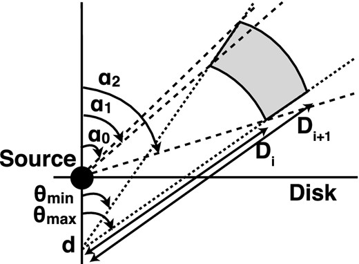
We follow the geometry of Sim et al. (2008, 2010a), where a biconical configuration as shown in Fig. 2 is adopted. This geometry was developed for studying radiative transfer in the wind of cataclysmic variables (Shlosman & Vitello 1993) and widely used for accretion disc winds (Knigge, Woods & Drew 1995; Sim et al. 2008, 2010a).
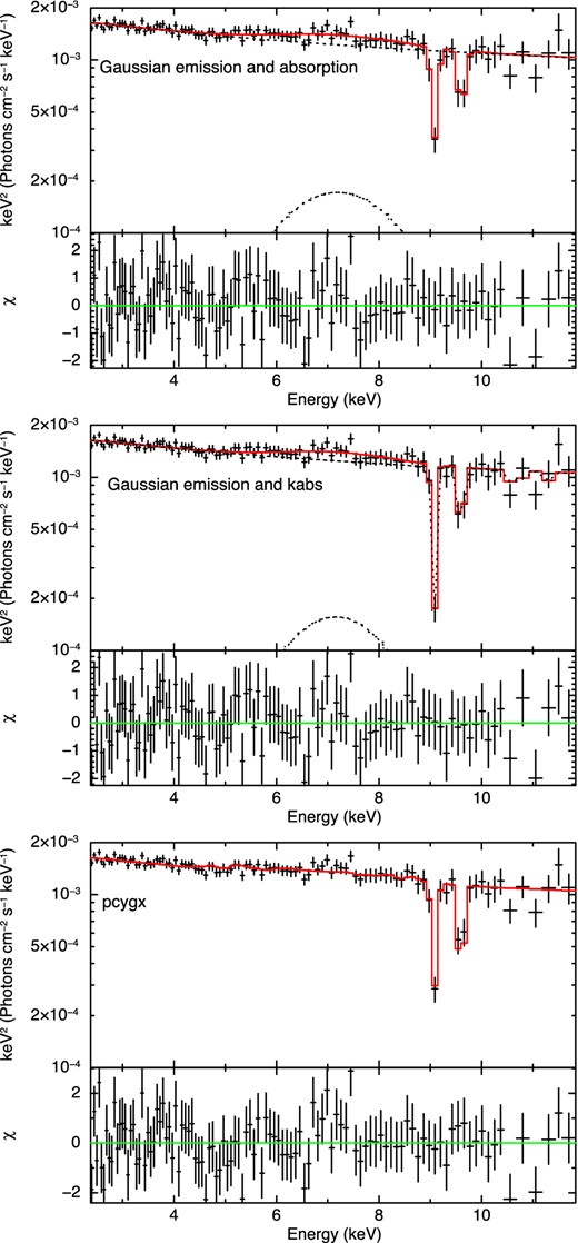
Suzaku spectra fitted with different parameters. Top: Gaussian emission and absorption, middle: kabs and Gaussian emission, bottom: pcygx. The spectra are shown in the rest frame of PDS 456.

Adopted geometry for our wind model and geometric variables. The shaded region is filled with outflowing materials. The wind is rotational symmetrical about z-axis.
This geometry is defined by three parameters. All stream lines in the wind converge at a focal point, which is at a distance d below the source. The wind is launched from Rmin to Rmax on the disc, We first assume that d = Rmin and Rmax = 1.5Rmin. This means that the wind fills a bicone between θmin = 45° and θmax = 56| $_{.}^{\circ}$|3 i.e. has solid angle Ω/4π = 0.15.
We define a mean launch radius R0 from the mean streamline i.e. it makes an angle of θ0 ≡ (θmin + θmax)/2. Thus, R0 = dtan θ0. The outer boundary of the wind geometry is assumed to be 5 × 1018 cm. As described in following sections, we chose Rmin = 20Rg ≃ 5.9 × 1015 cm for MBH = 2 × 10⁹ M⊙ (Reeves et al. 2009). Therefore, the outer boundary is three orders of magnitude larger than an inner radius Rmin. Thus, the density at the outer boundary is negligible compared with that at Rmin. The geometry is divided into 100 shells. Each shell has an equal width on a logarithmic scale. The radial and azimuthal velocity is assigned at a centre on a logarithmic scale for each shell.
3.1.2 Velocity and mass
3.1.3 Ionization calculation
A geometry used for ionization calculation.
An input spectrum for xstar should be defined in 1–1000 Ry (0.0136–13.6 keV) energy band. Although we do not know PDS 456 spectrum in the UV band, we extrapolate a simple power law with photon index Γ = 2.5. The ionization luminosity in this energy range is calculated from 2 to 10 keV X-ray luminosity. If we use Γ = 2.2, the ionization parameter log ξ decreases by 10–20 per cent.
xstar requires density n, luminosity L and ionization parameter log ξ = log (L/(nR2)) for input parameters. The density and luminosity are calculated by equations (6) and (10). To get the ionization parameter, the distance R is needed. Here, the distance R is defined to be a distance between the source and the inner edge of each shell. Additionally, we inputted a turbulent velocity calculated by equation (4). Atomic abundances are assumed to be equal to the solar abundances for all elements.
3.1.4 Three-dimensional radiative transfer
We use our Monte Carlo simulation code called monaco (Odaka et al. 2011) for the detailed radiative transfer. monaco is a general-purpose framework for synthesizing X-ray radiation from astrophysical objects by calculating radiative transfer based on the Monte Carlo approach. This framework utilizes the Geant4 toolkit library (Agostinelli et al. 2003; Allison et al. 2006) in order to calculate particle trajectories and physical interactions of the particles with matter in a complicated geometry. monaco is designed to treat astrophysical applications in which matter can form into an ionized plasma and can have motion that results in the Doppler shifts and broadenings. A variety of geometries and physical processes of photons are equipped and selectable for different astrophysical applications.
We have already included full treatment of photon processes related to an X-ray photoionized plasma. Detailed implementation of the physical processes is described in Watanabe et al. (2006). The simulation tracks photon interactions with ions, namely photoionization and photoexcitation; after these interactions reprocessed photons generated via recombination and atomic deexcitation are continue to be tracked. Compton scattering by free electrons is also taken into account. In this work, we consider only H- and He-like ions of Fe and Ni, and we ignore other ions. This assumption is justifiable by the fact that in the region of interest lighter elements are fully stripped, and L-shell ions of Fe and Ni with a few electrons have a small impact on the absorbed spectrum even if they exist.
We divide into 64 parts in azimuthal angle and 2 parts in polar angle since each cell can have only one velocity vector in this simulation code. Therefore, 100(radial) × 64(azimuthal) × 2(polar) cells are constructed in this Monte Carlo simulation. We populate this using a power-law spectrum with photon index Γ = 2.5 in the 5–200 keV energy range. Initial directions of the seed photons are limited to the upper half of the disc because photons below the disc usually cannot penetrate the disc.
3.2 Parameter choice
We translate the observational data above into appropriate simulation parameters. First, we assume a minimum turbulent velocity vturb,0 = 103 km s−1 (Reeves et al. 2009, 2014), and set v∞ = 0.3c (maximum velocity of H-like iron) This implies a launch radius of Rmin = 20Rg for |$v_{\infty }=v_{\rm esc}=c\sqrt{2R_{\rm g}/R}$|. We assume that this extends to Rmax = 1.5Rmin = 30Rg. We need the wind to be quite likely to intercept our line of sight in order to see absorption, so we assumed Ω/4π = 0.15 (Tombesi et al. 2013).
We assume that the wind is radiation driven, so we can get some idea of its polar angle from the ratio of luminosity from 20 to 30Rg, which will vertically accelerate the wind, to the luminosity from 6 to 20Rg which pushes the wind sideways (see e.g. Risaliti & Elvis 2010; Nomura et al. 2013). For a spin zero black hole accreting at L = LEdd, we find L(20–30Rg) = 0.64L(6–20Rg), giving a polar angle of ∼57°. Hence, we choose to fill the solid angle in a bicone from 45° to 56| $_{.}^{\circ}$|5 (Sim et al. 2010a,b).
Conservation of mass (equation 5) means n(R) ∝ 1/(vr(R)R2). The total column density along the wind is |$\int _{R_0}^{\infty } n(R) {\rm d}R$|, so for fast acceleration, where v(R) ∼ v∞ for all R then |$\dot{M}_{\rm wind}=4\pi v_{\infty } m_{\rm p} (\Omega /4\pi ) 1.23 N_{\rm H} R_{0}$|. The lower limit to the total hydrogen column (from the upper limit to the turbulent velocity) implies |$N_{\rm H}=(N_{\rm Fe\,\small {xxv}}+N_{\rm Fe\,\small {xxvi}}+N_{\rm Fe\,\small {xxvii}})/A_{\rm Fe}>1.5\times 10^{23}$| cm−2, so the absolute minimum mass-loss rate is |$\dot{M}_{\rm wind}\sim 0.5$| M⊙ yr−1 for Ω/4π = 0.15. Conversely, the upper limit to the column from the lowest velocity limit implies an upper limit to the mass-loss rate of ∼50 M⊙ yr−1, though it could be higher still if there is substantial material which is completely ionized and hence invisible. However, these larger columns have very large optical depth to electron scattering (τT = 1 corresponds to NH = 1.5 × 1024 which corresponds to 5 M⊙ yr−1), at which point the wind becomes self shielding, and radiative transfer within the wind would lead to low-ionization species which are not seen. Increasing the mass-loss rate increases the optical depth, to τ = 10 for 50 M⊙ yr−1. This would completely obscure the X-ray source along all directions which intercept the wind.
We can set an upper limit on the wind mass-loss by the mass accretion rate. We use the accretion disc code optxagnf (Done et al. 2012) with Galactic reddening of 0.48 (Simpson 2005) and simulate an accretion disc spectrum for a black hole of mass 2 × 10⁹ M⊙ yr−1. We match the observed B- and V-band fluxes (Ojha et al. 2009) for L = 0.4LEdd for a spin 0 black hole, i.e. a bolometric luminosity of ∼1047 erg s−1 and mass accretion rate of |$\dot{M}=31$| M⊙ yr−1. Alternatively, this gives L = 2LEdd for a spin 0.998, corresponding to Lbol ∼ 5 × 1047 erg s−1 and mass accretion rate of |$\dot{M}=27$| M⊙ yr−1. The lack of dependence of the derived mass accretion rate on black hole spin is as expected, as spin only affects the disc structure on size scales comparable to the last stable orbit, whereas the optical emission which we use to derive mass accretion rate is produced from further out in the disc. Clearly, the maximum mass-loss rate is then equal to the mass input rate of 30 M⊙ yr−1, but we set a conservative limit of 15 M⊙ yr−1, where we can lose up to half of the input mass accretion rate.
The density of the material is also determined by the opening angle of the wind with |$n(R) \propto \dot{M}_{\rm wind}/[R^2 v(R) (\Omega /4\pi )]$| (equation 5). A wider opening angle means that the wind is more likely to intercept the line of sight, but also means that the same mass-loss rate is spread into a larger volume, so this has lower density. This determines the ionization parameter |$\xi =L/(nR^2) \propto v(R) (\Omega /4\pi )/\dot{M}_{\rm wind}$|, which controls the ratio of H-like to H-like ion column density. The fact that the data (weakly) require He-like and H-like to have different velocities implies that the ionization is not constant in the wind as might be expected if all the absorption is produced after the wind has been accelerated to its terminal velocity (so v = v∞ and is constant). This shows that it is feasible to use observational data to constrain the wind acceleration.
We show results for |$\dot{M}=10$| M⊙ yr−1. We calculate the ionization using the measured 2–10 keV X-ray luminosity of 4 × 1044 erg s−1. The results for this for a series of inclination angles through the wind are shown in Fig. 4. The lines clearly increase in both equivalent width and intrinsic width at higher inclinations, and the ratio of H-like to He-like iron decreases.
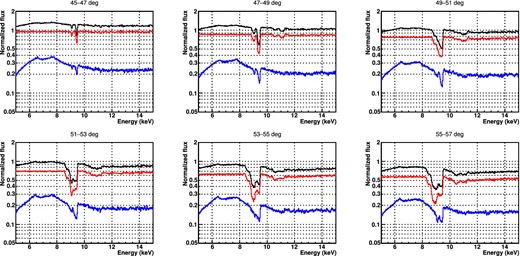
monaco spectra with L = 4 × 1044 erg s−1, |$\dot{M}=10$| M⊙, v0 = vturb = 1000 km s−1, β = 1 and Rmin = 20Rg. The direct component and reprocessed component are plotted in red and blue, respectively. The total spectrum is plotted in black. Y-axis is normalized to the input power-law spectrum.
Fig. 5 shows the ionization structure of the wind, with the lines of sight marked on it. At larger radii, the product of the density and the radius squared (nR2) is almost constant according to equation (5), due to the saturated velocity. Therefore, the H/He ratio shows a slight decrease, which is caused by the decrease of the luminosity due to the wind absorption. On the other hand, since the wind is still accelerating at the smaller radii, there is more He-like than H-like iron (see also Sim et al. 2008). As shown in the figure, the high-inclination line of sight includes material at smaller radii, where the wind is denser and less ionized. This gives the increase in equivalent width and more He-like than H-like iron.
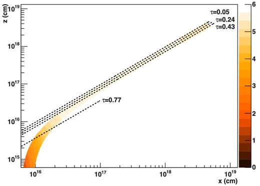
Ratio of H-like to He-like iron through the wind, together with the lines of sight for θincl = 46°, 50°, 54° and 70° for the same simulation as in Fig. 4, labelled with the total column density along that line of sight. Higher inclination samples material at smaller radii, where it is still accelerating so the density is higher hence the abundance of He-like iron is higher.
4 COMPARISON OF SIMULATIONS AND OBSERVATIONS
4.1 Absorption lines
The simulation above is close to the largest feasible mass outflow rate, so is close to the lowest possible ionization for the observed 2–10 keV X-ray luminosity of 4 × 1044 erg s−1 for the assumed launch radius of 20–30Rg and solid angle Ω/4π = 0.15. However, it is remarkably difficult to reproduce the observed absorption line equivalent and intrinsic widths from this, irrespective of the velocity law chosen, as the material is very highly ionized (so produces little He-like line) except at high-inclination angles. But at these high-inclination angles, the line of sight intercepts a large range of velocities, so the lines are broad and blend into each other rather than producing the two narrow lines seen in the data. Also, material at high inclination is somewhat shielded from the ionizing luminosity by the rest of the wind. Hence, it has lower ionization state, so at large inclinations, the He-like ion is produced preferentially at larger radii than the H-like ion, giving the He-like line a higher outflow velocity than the H-like, contrary to observations. Thus, both the narrow line width and the slightly higher velocity in H-like than He-like imply that the inclination angle through the wind is not too high, but low-inclination angles through the wind are too highly ionized, producing too small an equivalent width of He-like Fe for low-inclination angles through the wind, and too broad lines for higher inclination angles.
We show this by fitting the monaco model to the 6.5–10 keV data. We tabulate the model as multiplicative factors, and apply these to a power-law continuum with Galactic absorption. The monaco model has two free parameters of redshift z and inclination angle θincl. We allowed redshift to be free rather than fixing it to the cosmological redshift of z = 0.184 as this allows us to fit for slightly different wind velocity than is included in the simulation. The 6.5–10 keV spectrum is used in order to concentrate on the absorption lines. The best fit, shown in the left-hand panel of Fig. 6, is not very good, with χ2 = 32/27 in the 6.5–10 keV range. This is significantly worse than the phenomenological fits in Table 2. It is clear from the left-hand panel of Fig. 6 that the ionization state of this model is much higher than in the data.
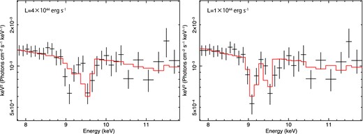
Left: Suzaku data and monaco spectrum with L = 4 × 1044 erg s−1, |$\dot{M}=10$| M⊙ yr−1, v0 = vturb = 1000 km s−1, β = 1 and Rmin = 20Rg. Best-fitting parameters are z = 0.165 ± 0.007 (v ≃ 0.315c), θincl = 49| $_{.}^{\circ}$|0 ± 0| $_{.}^{\circ}$|9 and Γ = 2.35(fix). Fit statistic is χ2 = 32.32/27. Right: same figure as the left-hand panel except with L = 1 × 1044 erg s−1. Best-fitting parameters are z = 0.174 ± 0.005 (v ≃ 0.308c), θincl = 47| $_{.}^{\circ}$|1 ± 0| $_{.}^{\circ}$|4 and Γ = 2.35(fix). Fit statistic is χ2 = 21.48/27. All spectra are shown in the rest frame of PDS 456.
Changing the velocity law does not substantially change this conclusion. A much higher initial velocity v0 = 0.15c gives a slightly better fit as this means that the higher inclination lines of sight through the wind intercept a smaller range of velocity, so the lines are narrower. Similarly, decreasing β also gives a more homogeneous velocity structure as then most of the acceleration happens very close to the disc. Full results for these two cases are shown in the Appendix, but none of these give a particularly good fit to the data, with χ2 > 33/27 for the 6.5–10 keV bandpass.
Increasing the distance at which the wind is launched gives a lower ionization parameter. The UV-line driven disc wind models of Risaliti & Elvis (2010) have v∞/v(R0)esc ∼ a few, at which point the wind could be launched at Rmin ∼ 50Rg. However, the ratio of accretion power at this point to the total accretion power is small, so such a wind would be expected to be more equatorial if it is driven by radiation as the ratio of luminosity under the wind pushing it up L(50–75Rg) is much smaller compared to L(6–50Rg) which is the radiation from the inner disc pushing it outwards.
We cannot reduce the ionization by shielding the gas, as we observe Lx = 4 × 1044 erg s−1 on our line of sight through the wind, so the wind also should see this luminosity. However, the outflow velocity is high enough that the X-ray luminosity as seen in the rest frame of the wind is substantially reduced by Doppler de-boosting, so that Lobs = Lxδ3+α ≈ 0.25Lx, where δ = [γ(1 − βcos θ)]−1 ≈ 0.73 (see appendix A3 of Schurch & Done 2007). Thus, the ionizing luminosity as seen by the wind varies from 4 to 1 × 1044, depending on the velocity of the wind. Since the data show that the majority of the absorption takes place at v ∼ v∞, we use an ionizing luminosity of 1044 erg s−1.
We re-simulate the wind over a range of parameters with this ionizing luminosity. The full simulation results are shown in Figs 7 and 8, showing clearly that the ionization state is lower, as expected.
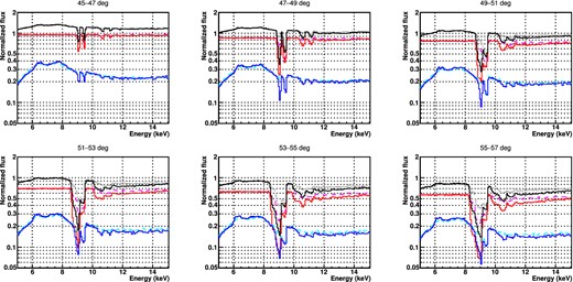
Dependence on the ionizing luminosity. The grey, magenta and cyan lines show the fiducial parameter simulation with L = 4 × 1044 erg s−1, |$\dot{M}=10$| M⊙ yr−1, while the black, red and blue dashed curves show the same parameters except with an ionizing luminosity L = 1 × 1044 erg s−1.

We fit this model to the data, with the best fit shown in the right-hand panel of Fig. 6. This is a better fit, as expected, with fit statistic of 21.5/27, which is not significantly different to the phenomenological fits in Table 2. We also simulated with |$\dot{M}=15$|, 8, 3, 1 M⊙ yr−1. Although 15 and 8 M⊙ yr−1 give comparably good fits, lower wind outflow rates give increasingly poor fits (χ2 = 28 and 51, respectively) as the absorption lines become too weak as the material is too highly ionized.
4.2 Emission lines from the wind
We now re-simulate the best monaco fit to the absorption lines shown in the right-hand panel of Fig. 6 over an extended energy grid from 2 to 200 keV. This enables us to look also at the emission lines produced by the wind. Fig. 9 shows the best fit comparison of this simulation with the 2–10 keV Suzaku data, where the monaco data are again incorporated as a multiplicative model. The fit parameters are power-law index and normalization, and the redshift is fixed at z = 0.174 (v∞ ≃ 0.308c). This gives χ2 = 106.5/105, which is not significantly worse than the phenomenological fits in Table 2 due to the smaller number of free parameters. For example, the model using kabs absorption lines with a broad Gaussian emission line has χ2 = 91.7/98, a difference of Δχ2 = 15 for seven additional degrees of freedom. This gives F = 15/7 which is 2.1, which is only better at 96 per cent confidence.

Suzaku data and monaco spectrum in 2–10 keV band with L = 1 × 1044 erg s−1, |$\dot{M}=10$| M⊙ yr−1, v0 = vturb = 1000 km s−1, β = 1 and Rmin = 20Rg. Best-fitting parameters are θincl = 47| $_{.}^{\circ}$|3 ± 0| $_{.}^{\circ}$|4 and Γ = 2.33 ± 0.01, and the redshift is fixed at z = 0.174 (v ≃ 0.308c). Fit statistic is χ2 = 106.49/105.
Unlike absorption, the line is emitted from the wind at all azimuths, and at all radii. Where the wind has already reached its terminal velocity, it has also expanded enough that its azimuthal velocity is small compared to its radial outflow velocity. Thus, the projected velocity in our line of sight ranges from −v∞ (θ = 0, along our line of sight as we look through the wind) to −v∞cos (θincl + θmax) ∼ −v∞cos 2θ0 giving a corresponding line energy of 6.04–9.13 keV for the 6.7 keV line while the 6.95 keV H-like extends from 6.26 to 9.47 keV for this simulation.
Thus, the maximum red extension of the emission line can give direct information on the opening angle of the wind. However, this is difficult to measure as the line is very broad, and the discussion above neglects the emission from the wind at small radii where the initially Keplarian azimuthal velocity is important. This line emission from small radii could have a larger projected velocity with |$-v_{\phi _0} \cos (\theta _{\rm incl}+90^\circ )\simeq (v_\infty /\sqrt{2}) \sin (\theta _{\rm incl})$| at maximum, giving a red extension at ∼5.7 keV for the He-like line. Our model shows that the red wing extends down to 6.0–6.3 keV (Fig. 9). This would be better matched to the data if it happened at 6.5–6.7 keV, so we experiment with different θmin but keep the same solid angle of the wind. We get better fit for a wind with θmin = 35° (Fig. 10) but the decrease in χ2 is not significant as these features are all small.
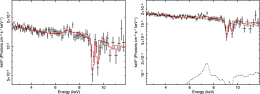
Left: Suzaku data and monaco spectrum in 2–10 keV band with L = 1 × 1044 erg s−1, |$\dot{M}=10$| M⊙ yr−1, v0 = vturb = 1000 km s−1, β = 1, Rmin = 20Rg and θmin = 35°. Best-fitting parameters are θincl = 37| $_{.}^{\circ}$|4 ± 0| $_{.}^{\circ}$|4, Γ = 2.30 ± 0.01, and the redshift is fixed at z = 0.174 (v ≃ 0.308c). Fit statistic is χ2 = 103.62/105. Right: Suzaku data and monaco spectrum with blurred disc reflection in 2–10 keV band with L = 1 × 1044 erg s−1, |$\dot{M}=10$| M⊙ yr−1, v0 = vturb = 1000 km s−1, β = 1, Rmin = 20Rg and θmin = 55°. Best-fitting parameters are θincl = 56| $_{.}^{\circ}$|8 ± 0| $_{.}^{\circ}$|3, Γ = 2.40 ± 0.04 and reflection fraction R ≃ 0.27, and the redshift is fixed at z = 0.174 (v ≃ 0.308c). Fit statistic is χ2 = 103.91/104. We changed the y-axis scale to show the reflected spectrum. All spectra are shown in the rest frame of PDS 456.
4.3 Emission lines from the wind and reflection from the disc
While the wind produces broadened emission lines from the H- and He-like material in the wind, the disc should also contribute to the emission via reflection. In our geometry, the disc still exists from 20Rg down to the innermost stable circular orbit. Hence, we include neutral reflection (pexmon) from this inner disc, with relativistic blurring from kdblur with outer radius fixed at 20Rg, inner radius fixed at 6Rg and emissivity fixed at 3. We assume that the inclination angle for both pexmon and kdblur is tied to inclination angle of the wind model. We obtained fit statistics of 103.62, 105.69, 103.91, 107.93 and 111.16, with reflection fractions of 1 × 10⁻³, 0.15, 0.27, 0.30 and 0.35 for respective values of θmin = 35°, 45°, 55°, 65°, 75°. We show the fit with θmin = 55° as this allows a contribution from the inner disc reflection, as expected. The spectrum is shown in the right-hand panel of Fig. 10.
5 APPLICATION TO THE OTHER OBSERVATIONS
We also applied our monaco models to the Suzaku data observed on 2011 March 16, 2013 February 21, 2013 March 3 and 2013 March 8 (Table 1). Hereafter, we refer to the data as 2011, 2013a,b and c, respectively. The data were processed and grouped in the same way as the 2007 data. The total net exposure times are 125.5, 182.3, 164.8 and 108.3 ks, respectively.
Fig. 11 shows the fluxed spectra of all Suzaku observations. The spectra show a large variability in both the continuum shape and Fe absorption lines. At first sight this variability appears correlated, with strongest absorption lines in the hardest spectra. We first assess the extent of the correlation of the absorption with spectral shape using phenomenological models, and then fit using the monaco spectra.
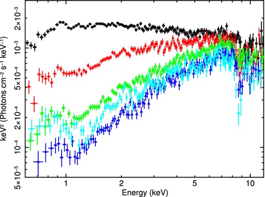
Suzaku XIS FI spectra from 2007 (black circle), 2011 (red cross), 2013a (green square), b (blue diamond) and c (cyan triangle), unfolded against Γ = 2 power law. All spectra are shown in the rest frame of PDS 456.
5.1 Spectral fitting with kabs model
Here, we assume that the intrinsic spectral shape is same as the 2007 observation, and only additional absorption makes spectral difference. Hence, we model the continuum spectra by a power-law model with photon index Γ = 2.35 and an ionized partial covering absorber zxipcf. Additional Fe absorption lines are modelled with kabs models. The best-fitting parameters are listed in Table 3 and the spectra are shown in Fig. 12.
Suzaku spectra fitted with kabs*zxipcf*powerlaw.
Spectral parameters for all Suzaku observations.
| Model component | Fit parameter | Value (90 per cent error) | |||
|---|---|---|---|---|---|
| 2011 | 2013a | 2013b | 2013c | ||
| Partial covering absorber | NH (1022 cm−2) | |$1.33^{+7.83}_{-1.03}$| | |$23.27^{+5.90}_{-7.00}$| | |$13.67^{+2.80}_{-3.70}$| | |$10.90^{+2.47}_{-5.62}$| |
| log ξ | −0.74( < 2.35) | |$2.35^{+0.16}_{-0.20}$| | |$2.01^{+0.17}_{-0.70}$| | |$1.92^{+0.26}_{-0.59}$| | |
| fcov | 0.78( > 0.33) | |$0.87^{+0.12}_{-0.08}$| | 1.00( > 0.90) | 0.89( > 0.84) | |
| Power law | Γ | 2.35 (fix) | |||
| |$F_\mathrm{2{\rm -}10\, keV}$| (10−12 erg s−1 cm−2) | |$3.14^{+0.36}_{-0.47}$| | |$3.27^{+0.43}_{-0.21}$| | |$2.45^{+0.16}_{-0.19}$| | |$2.21^{+0.30}_{-0.49}$| | |
| |$L_\mathrm{2{\rm -}10\, keV}$| (1044 erg s−1) | |$2.93^{+0.34}_{-0.44}$| | |$3.06^{+0.40}_{-0.20}$| | |$2.29^{+0.15}_{-0.18}$| | |$2.07^{+0.28}_{-0.46}$| | |
| Fe xxv Heα | vout | |$0.248^{+0.007}_{-0.007}c$| | |$0.224^{+0.035}_{-0.019}c$| | |$0.250^{+0.009}_{-0.009}c$| | |$0.223^{+0.014}_{-0.021}c$| |
| kT (keV) | 474 (fix) | 474 (fix) | 2391( < 46 431) | 11503( < 38 843) | |
| Natom (1018) | |$2.33^{+7.00}_{-1.47}$| | 1.01( < 2.02) | |$2.48^{+3.48}_{-1.31}$| | 2.08( < 6.42) | |
| EW (keV) | 0.088 | 0.057 | 0.135 | 0.125 | |
| Fe xxvi Lyα | vout | Tied to Fe xxv | |||
| kT (keV) | Tied to Fe xxv | ||||
| Natom (1018) | |$6.19^{+24.14}_{-4.25}$| | 0.59( < 3.72) | |$4.00^{+21.09}_{-2.96}$| | 11.98( < 20.41) | |
| EW (keV) | 0.101 | 0.025 | 0.126 | 0.232 | |
| Emission | LineE (keV) | |$6.35^{+0.57}_{-1.29}$| | |$7.54^{+0.24}_{-0.22}$| | |$7.49^{+0.20}_{-0.18}$| | |$7.08^{+0.47}_{-0.82}$| |
| σ (keV) | |$1.43^{+1.15}_{-0.53}$| | |$0.87^{+0.27}_{-0.23}$| | |$0.82^{+0.29}_{-0.20}$| | |$1.19^{+1.00}_{-0.52}$| | |
| EW (keV) | 0.605( < 1.152) | |$0.667^{+0.423}_{-0.218}$| | |$0.762^{+0.320}_{-0.234}$| | |$0.734^{+0.757}_{-0.709}$| | |
| Fit statistics | χ2/dof | 82.85/90 | 80.72/95 | 87.35/88 | 85.40/82 |
| Null probability | 0.69 | 0.85 | 0.50 | 0.38 | |
| χ2/dof for 6.5–10.0 keV | 19.81/13 | 12.84/18 | 13.02/11 | 2.26/5 | |
While the absorption lines are indeed strongest in one of the spectra with the strongest low energy absorption (2013c, cyan in Fig. 12) there is not a one-to-one correlation. The equivalent widths of absorption lines vary by more than a factor of 2 in 2013 data, while the continuum absorption is rather similar (2013a,b and c i.e. green blue and cyan in Fig. 12). Conversely, the absorption line equivalent width in 2013a (green in Fig. 12) is significantly less than that in the 2007 (unabsorbed) data. Thus, the continuum shape change is not directly correlated with the wind, and is hence is unlikely to arise from a decrease in the ionization state of the entire wind structure. Instead, it more probably represents an additional absorbing cloud along the line of sight.
This cloud could be either be between the continuum source and the wind i.e. the wind also sees the same change in illuminating spectrum as we do, or it could be between the wind and us, in which case the wind sees the original, unabsorbed ionizing continuum. We use xstar to see if the data can distinguish between these two absorber locations. However, the observed H-like to He-like ratio is mainly determined by hard X-ray illumination, and this is not dramatically changed by the absorber. Hence, the current data are not able to locate the additional absorption, and so we assume that it is outside of the wind, and that the wind sees the unobscured continuum.
We note that similar, long lived, external absorption is clearly seen in NGC 5548 (Kaastra et al. 2014), though this is typically much lower ionization with log ξ ∼ −0.5 compared to the log ξ ∼ 2 required by the 2013 data. This higher ionization is caused by Kα (∼6.4 keV) and Kβ (∼7.1 keV) absorption lines from moderately ionized Fe ions, which are (marginally) seen in our data (see Fig. 12).
5.2 Monaco Simulations
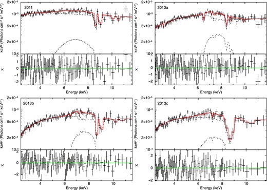
In order to determine the simulation parameters, we compared the 6.5–10.0 keV spectra of the observations between 2011 and 2013 with the model with L = 1 × 1044 erg s−1, v∞ = 0.3c, v0 = vturb = 1000 km s−1, β = 1 and Rmin = 20Rg. We optimize three parameters of mass outflow rate |$\dot{M}_{\rm wind}$|, inclination angle θincl and wind velocity vout. Since vout works like redshift z for absorption lines, we use z instead of vout. We simulate four grids of mass outflow rates, 15, 10, 8 and 3 M⊙ yr−1. The geometrical parameter θmin is fixed at 45° because it does not have large effect on the absorption line features.
As the results, the fit statistics are best with |$\dot{M}_{\rm wind}=8$|, 10, 8, 10 M⊙ yr−1, respectively, for 2011, 2013a, 2013b and 2013c observations. Although |$\dot{M}_{\rm wind}=8$|, 10, 15 M⊙ yr−1 gives comparably good fit for any observations, we choose the best-fitting value of |$\dot{M}_{\rm wind}$|. For these mass outflow rates, the best-fitting values of redshift are z = 0.232, 0.267, 0.218, 0.238, respectively, which corresponds to v = 0.263 ± 0.006c, 0.237 ± 0.008c, 0.274 ± 0.006c and 0.259 ± 0.007c. Here, the obtained values of mass outflow rate should be corrected by the outflow velocity because the outflow velocity is assumed to be 0.3c in the simulations. According to equation (5), the mass outflow rate |$\dot{M}$| is proportional to the density n and the outflow velocity v as |$\dot{M}\propto nv$|. Since the density determines the ionization structure and the absorption column, the density in the simulation nsim has to equal to that in the observed spectra nobs. Thus, the corrected mass outflow rate is |$\dot{M}_{\rm obs}\simeq \dot{M}_{\rm sim}v_{\rm obs}/v_{\rm sim}$|, and the best-fitting values of the mass outflow rate become |$\dot{M}_{\rm wind}\simeq 7$|, 8, 7, 9 M⊙ yr−1, respectively. For the absorption lines, the change of inclination angle is interpreted as the change of opening angle of the wind and/or change of θmin. Here, it is assumed that the geometrical parameter θmin equals to 45° in the 2007 observation.
The comparison between the observed spectra and our simulation models is shown in Fig. 13. All simulation parameters are listed in Table 4. The observed time variability of the wind could be caused by the hydrodynamic instability of a UV-line driven disk wind as seen in Proga & Kallman (2004) and Nomura (2014). Variability of the wind on even shorter time-scales is discussed by Gofford et al. (2014).
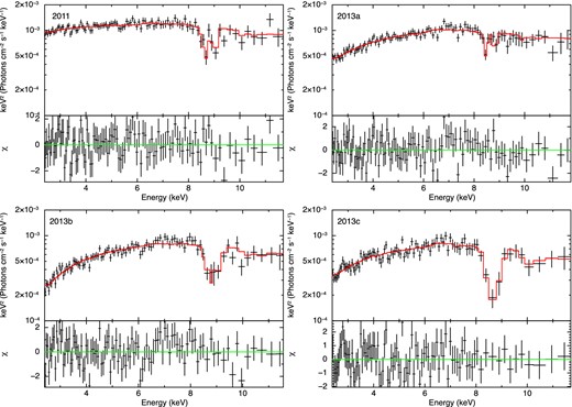
monaco model and Suzaku spectra for 2011, 2013a, 2013b and 2013c. All spectra are shown in the rest frame of PDS 456.
monaco parameters for all Suzaku observations.
| Parameter | Value | |||||
|---|---|---|---|---|---|---|
| 2007 | 2011 | 2013a | 2013b | 2013c | ||
| monaco wind | |$\dot{M}_{\rm wind}$| (M⊙ yr−1) | 10 | 7 | 8 | 7 | 9 |
| vout | 0.308ca | 0.263c | 0.237c | 0.274c | 0.259c | |
| θmin | 45° | 43| $_{.}^{\circ}$|6 | 45| $_{.}^{\circ}$|7 | 41| $_{.}^{\circ}$|6 | 40| $_{.}^{\circ}$|6 | |
| θincl | |${47.3^{+0.7}_{-0.6}}^\circ$| | |${48.6^{+1.1}_{-0.9}}^\circ$| | |${47.3^{+0.8}_{-1.6}}^\circ$| | |${48.0^{+1.3}_{-1.2}}^\circ$| | |${48.4^{+1.6}_{-1.4}}^\circ$| | |
| Continuum spectra | NH (1022 cm−2) | – | |$4.1^{+11.1}_{-1.1}$| | |$6.0^{+5.5}_{-1.8}$| | |$5.0^{+1.4}_{-1.1}$| | |$9.9^{+6.4}_{-5.4}$| |
| log ξ | – | −0.57( < 2.28) | −0.39( < 0.31) | −0.85( < −0.26) | 0.27( < 1.82) | |
| fcov | – | |$0.56^{+0.07}_{-0.12}$| | |$0.78^{+0.06}_{-0.09}$| | |$0.91^{+0.07}_{-0.08}$| | |$0.75^{0.13}_{-0.03}$| | |
| Γ | |$2.33^{+0.02}_{-0.02}$| | 2.35 (fix) | ||||
| Fit statistics | χ2/dof | 106.49/105 | 89.20/95 | 102.40/100 | 105.41/94 | 89.07/88 |
| Null probability | 0.44 | 0.65 | 0.41 | 0.20 | 0.45 | |
| χ2/dof for 6.5–10.0 keV | 21.86/27 | 24.08/18 | 21.22/23 | 19.33/17 | 3.44/11 | |
aWe simulate with vout = 0.3c, and then shift the spectrum.
6 DISCUSSION
Table 4 shows that the best-fitting values of mass outflow rate of winds in PDS 456 of |$\dot{M}_{\rm wind}\simeq 7$|–10 M⊙ yr−1, roughly 30 per cent of the total mass inflow rate as traced by the optical emission from the outer disc. The kinetic energy and momentum of the wind are close to that provided by the radiation field (Gofford et al. 2013, 2014), pointing to the importance of radiative driving in launching and accelerating the wind. However, the mechanism for this is unclear. UV-line driving results in powerful winds from the UV bright O stars and disc accreting white dwarfs, but the X-rays which accompany the bright UV discs in AGN strongly suppress the wind through overionization (Proga & Kallman 2004). The ultrafast outflow (UFO)'s are so highly ionized that there is no UV or even soft X-ray opacity left, so UV line driving cannot be accelerating the highly ionized material which we see (Higginbottom et al. 2014).
However, here we suggest a solution to this issue. UV line driving could be launching and accelerating the material from the disc. As it rises higher it is pushed outwards and ionized by the harder UV and X-ray radiation from the inner disc. The UV opacity in then mostly on the vertically rising part of the wind, which is outside of our line of sight (see e.g. the wind geometries in Risaliti & Elvis 2010; Nomura et al. 2013).
We can estimate the effect of this in PDS 456. Without mass-loss, such a disc should have L(20–30Rg) = 0.64L(6–20Rg), so reducing the inner disc luminosity by 2/3 to account for the smaller mass accretion rate gives L(20–30Rg) ≈ L(6–20Rg). Assuming that the wind is launched vertically by the disc luminosity from 20 − 30Rg, and pushed sideways by the inner disc luminosity from 6 to 20Rg gives an estimate for θ0 ∼ 45°, the angle the wind makes to the disc normal. This is even more convincingly close to our fiducial geometry than with the standard (no mass-loss in a wind) disc (see Section 3.2).
Laor & Davis (2014) have done a much more exact calculation of the effect of mass-loss on the disc structure. Their models include the energy to power the wind to its local escape velocity (ϵ = 1) on the structure of the remaining disc, as well as the effect of angular momentum losses and decrease in mass accretion rate. They parametrize the mass-loss rate from each surface element of the disc by using observed O star winds i.e. they assume that the winds are UV line driven, and scale for the different gravity (g) conditions. This gives a surface density mass-loss rate of |$\dot{\Sigma }\propto F^{2.32}/g^{1.11}$|, where F ∝ T4 is the local surface flux. However, O stars only span a rather small range in temperature, from 2.8to5 × 104 K (Howarth & Prinja 1989), so this relation only formally holds for this range. None the less, this is close to the disc temperatures expected for such a high-mass black hole, so the Laor & Davis (2014) results should be applicable. Table 5 shows the full numerical calculation of UV-line driven winds (Davis, private communication). This calculation is done for 109 M⊙ black hole for a★ = 0 and 0.9, accreting at L/LEdd = 0.3 and 1. These show that mass-loss rates of 30–50 per cent of the mass inflow rate are expected from UV-line driven disc winds assuming that the central X-ray flux does not overionize the wind.
Full numerical calculation of UV-line driven winds. All accretion rates are in units of the Eddington accretion rate.
| L/LEdd | aa | |$\dot{M}_{\rm in}$|b | |$\dot{M}$|c | |$\dot{M}_{\rm wind}$|d |
|---|---|---|---|---|
| 0.3 | 0 | 0.302 | 0.515 | 0.21 |
| 0.9 | 0.302 | 1.174 | 0.87 | |
| 1.0 | 0 | 1.007 | 2.282 | 1.09 |
| 0.9 | 1.007 | 5.588 | 4.58 |
| L/LEdd | aa | |$\dot{M}_{\rm in}$|b | |$\dot{M}$|c | |$\dot{M}_{\rm wind}$|d |
|---|---|---|---|---|
| 0.3 | 0 | 0.302 | 0.515 | 0.21 |
| 0.9 | 0.302 | 1.174 | 0.87 | |
| 1.0 | 0 | 1.007 | 2.282 | 1.09 |
| 0.9 | 1.007 | 5.588 | 4.58 |
aBlack hole spin parameter.
bThe amount of mass that is actually accreted.
cThe accretion rate at large radius before the outflow set in.
dMass outflow rate.
The X-ray power then becomes critically important, and AGN are observed to show an anticorrelation of X-ray flux with L/LEdd (Vasudevan & Fabian 2007; Done et al. 2012; Jin et al. 2012a; Jin, Ward & Done 2012b; see their figs 8a and b). While the underlying reason for this is not well understood, it is clear that as a source approaches LEdd, then radiation pressure alone means that winds become important, while the drop in X-ray luminosity means that UV line driving becomes more probable since the X-ray ionization drops. This combination of continuum and UV line driving seems the most likely way to drive the most powerful winds.
This predicts that fast winds should be suppressed in lower L/LEdd objects, as L/LEdd ≪ 1 means that the wind cannot be powered by continuum driving (definition of the Eddington limit) and the higher X-ray flux means that UV line driving is strongly suppressed. It also predicts that the fastest winds should be seen in the highest mass objects with L/LEdd ∼ 1 as these are the ones where the disc luminosity peaks in the UV rather than the far-UV/soft X-rays, where the disc itself contributes to overionizing the wind. Fig. 14 shows the predicted spectral energy distributions for L/LEdd = 1 for Schwarzchild black holes of mass 106 (blue) and 109 M⊙ (red). These assume that the accretion energy is dissipated in a standard (constant mass inflow rate) disc, and thermalizes to a (colour temperature corrected) blackbody down to 10Rg, and that 30 per cent of the accretion energy below this powers a tail to high energies with Γ = 2.4, while the remainder powers a low temperature, optically thick corona (kTe = 0.2, τ = 15: see Done et al. 2012). The black vertical line marks the 13.6 eV Hydrogen ionization point. A blackbody at O star temperatures will peak in the 10–18 eV range, so this indicates the UV-line driving bandpass. Clearly, the disc for the more massive black hole will have much stronger UV line driving that the less massive one. Simply assigning all of the disc luminosity to a UV band as is often done in hydrodynamic calculations to make them numerically tractable (Proga & Kallman 2004; Nomura 2014) does not include this mass dependence, so may overestimate the wind mass-loss rates for lower mass AGN (e.g. Laor & Davis 2014).
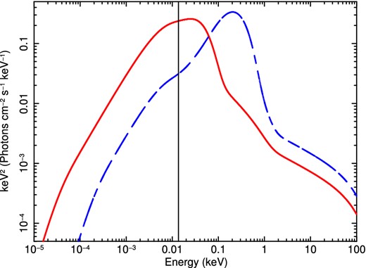
Predicted spectral energy distributions for spin zero black holes of mass 106 (blue dashed) and 109 M⊙ (red). The black vertical line is at 13.6 eV hydrogen ionization point which corresponds to the UV-line driving bandpass. Here, we use optxagnf (Done et al. 2012) and assume L/LEdd = 1.
Thus, we expect the most powerful winds to be powered by a combination of continuum and UV line driving, and for these winds to be found in the most massive AGN. This is clearly the case, with the winds in PDS 456 and APM 08279+5255, both high-mass (>109 M⊙) black holes at L ∼ LEdd, standing out as by far the highest velocity, highest mass-loss rate objects (Tombesi et al. 2010; Gofford et al. 2013). We will fit the wind in APM 08279+5255 in a subsequent paper. Please note that we can say nothing about the magnetic driving in this paper. As well as the radiative driving, the magnetic driving also need to be explored further.
7 CONCLUSIONS
We show that the geometry and energetics of wind in PDS 456 can be constrained using our new combined Monte Carlo and ionization code, monaco. The code treats only H and He-like ions, but this makes it fast enough that we can explore parameter space for highly ionized winds, where this approximation is appropriate.
Our simulations successfully reproduce all the Suzaku observations of PDS 456. In particular, we can explain the time variability of the wind spectra within several weeks observed in 2013 in our modelling framework. Most of the fundamental parameters are kept constant in our simulations but wind velocity and relative angle between the line of sight and wind direction are sightly changed.
From our simulations, we find that the best-fitting values of mass outflow rate of winds in PDS 456 are 7–10 M⊙ yr−1, corresponding to ∼30 per cent of the total mass inflow rate. According to full numerical calculation of UV-line driven winds done by Laor & Davis, these results can match the properties of UV-line driven disc wind models. The wind is vertically accelerated by the UV emission from the disc before it is pushed sideways by the inner disc emission and ionized by the central X-ray source. This mechanism works most efficiently in high-mass AGN, as their discs peak in the UV. Observations also show that as AGN approach Eddington, the fraction of X-ray luminosity decreases. This helps the wind not to be overionized, as well as giving extra acceleration to the wind from continuum radiation driving. Thus the most extreme outflows are predicted to be observed in high-mass, high Eddington fraction AGN.
CD thanks Shane Davis for the calculations of the UV-line driven disc winds shown in Section 6, and for multiple useful conversations about discs and winds. KH is supported by the Japan Society for the Promotion of Science (JSPS) Research Fellowship for Young Scientists. We thank the referee for their comments which improved the structure of the paper.
REFERENCES
SUPPORTING INFORMATION
Additional Supporting Information may be found in the online version of this article:
Appendix A. Parameter dependence (Supplementary Data).
Please note: Oxford University Press is not responsible for the content or functionality of any supporting materials supplied by the authors. Any queries (other than missing material) should be directed to the corresponding author for the paper.
