The intimate relation between the low T/W instability and the corotation point Free

Key quantities for three sequences of differentially rotating equilibrium configurations. The stellar models are described by a γ = 2 polytropic EoS and the j-constant rotation law. The first column gives the parameter A that controls the degree of differential rotation. In the second and third columns, we provide, respectively, the ratio of polar to equatorial axes and the parameter j₀. The mass, maximum pressure, angular momentum and the rotational parameter β = T/|W| are given in the last four columns, respectively. All quantities are expressed in dimensionless units, where G is the gravitational constant, ρ_m represents the maximum mass density and R_eq is the equatorial radius.

A/R_eq	R_p/R_eq	\|$j_{0} / (\sqrt{G\rho _{\rm m}} R_{\rm eq}^2)$\|	\|$M / (\rho _{\rm m} R_{\rm eq}^3)$\|	\|$p_m /(G R_{\rm eq}^2 \rho _{\rm m} ^2)$\|	\|$J /(G^{1/2} \rho _{\rm m} ^{3/2} R_{\rm eq}^5)$\|	β × 10²
1.0	1.0	0.000	1.273	0.637	0.000	0.00
1.0	0.9	0.569	1.167	0.570	0.125	2.49
1.0	0.7	0.964	0.947	0.431	0.174	8.36
1.0	0.5	1.189	0.718	0.285	0.165	15.82
1.0	0.3	1.337	0.558	0.149	0.152	25.57
0.5	0.9	0.231	1.229	0.585	0.125	2.33
0.5	0.7	0.413	1.161	0.474	0.219	7.72
0.5	0.5	0.547	1.116	0.359	0.294	14.07
0.5	0.3	0.605	0.997	0.259	0.318	20.05
0.5	0.1	0.593	0.891	0.209	0.299	22.43
0.1	0.9	0.049	1.329	0.623	0.059	0.80
0.1	0.7	0.091	1.356	0.592	0.114	2.53
0.1	0.5	0.121	1.355	0.559	0.152	4.23
0.1	0.3	0.143	1.344	0.531	0.531	5.59
0.1	0.1	0.154	1.336	0.515	0.193	6.36

A/R_eq	R_p/R_eq	\|$j_{0} / (\sqrt{G\rho _{\rm m}} R_{\rm eq}^2)$\|	\|$M / (\rho _{\rm m} R_{\rm eq}^3)$\|	\|$p_m /(G R_{\rm eq}^2 \rho _{\rm m} ^2)$\|	\|$J /(G^{1/2} \rho _{\rm m} ^{3/2} R_{\rm eq}^5)$\|	β × 10²
1.0	1.0	0.000	1.273	0.637	0.000	0.00
1.0	0.9	0.569	1.167	0.570	0.125	2.49
1.0	0.7	0.964	0.947	0.431	0.174	8.36
1.0	0.5	1.189	0.718	0.285	0.165	15.82
1.0	0.3	1.337	0.558	0.149	0.152	25.57
0.5	0.9	0.231	1.229	0.585	0.125	2.33
0.5	0.7	0.413	1.161	0.474	0.219	7.72
0.5	0.5	0.547	1.116	0.359	0.294	14.07
0.5	0.3	0.605	0.997	0.259	0.318	20.05
0.5	0.1	0.593	0.891	0.209	0.299	22.43
0.1	0.9	0.049	1.329	0.623	0.059	0.80
0.1	0.7	0.091	1.356	0.592	0.114	2.53
0.1	0.5	0.121	1.355	0.559	0.152	4.23
0.1	0.3	0.143	1.344	0.531	0.531	5.59
0.1	0.1	0.154	1.336	0.515	0.193	6.36

Table 1.

Key quantities for three sequences of differentially rotating equilibrium configurations. The stellar models are described by a γ = 2 polytropic EoS and the j-constant rotation law. The first column gives the parameter A that controls the degree of differential rotation. In the second and third columns, we provide, respectively, the ratio of polar to equatorial axes and the parameter j₀. The mass, maximum pressure, angular momentum and the rotational parameter β = T/|W| are given in the last four columns, respectively. All quantities are expressed in dimensionless units, where G is the gravitational constant, ρ_m represents the maximum mass density and R_eq is the equatorial radius.

A/R_eq	R_p/R_eq	\|$j_{0} / (\sqrt{G\rho _{\rm m}} R_{\rm eq}^2)$\|	\|$M / (\rho _{\rm m} R_{\rm eq}^3)$\|	\|$p_m /(G R_{\rm eq}^2 \rho _{\rm m} ^2)$\|	\|$J /(G^{1/2} \rho _{\rm m} ^{3/2} R_{\rm eq}^5)$\|	β × 10²
1.0	1.0	0.000	1.273	0.637	0.000	0.00
1.0	0.9	0.569	1.167	0.570	0.125	2.49
1.0	0.7	0.964	0.947	0.431	0.174	8.36
1.0	0.5	1.189	0.718	0.285	0.165	15.82
1.0	0.3	1.337	0.558	0.149	0.152	25.57
0.5	0.9	0.231	1.229	0.585	0.125	2.33
0.5	0.7	0.413	1.161	0.474	0.219	7.72
0.5	0.5	0.547	1.116	0.359	0.294	14.07
0.5	0.3	0.605	0.997	0.259	0.318	20.05
0.5	0.1	0.593	0.891	0.209	0.299	22.43
0.1	0.9	0.049	1.329	0.623	0.059	0.80
0.1	0.7	0.091	1.356	0.592	0.114	2.53
0.1	0.5	0.121	1.355	0.559	0.152	4.23
0.1	0.3	0.143	1.344	0.531	0.531	5.59
0.1	0.1	0.154	1.336	0.515	0.193	6.36

A/R_eq	R_p/R_eq	\|$j_{0} / (\sqrt{G\rho _{\rm m}} R_{\rm eq}^2)$\|	\|$M / (\rho _{\rm m} R_{\rm eq}^3)$\|	\|$p_m /(G R_{\rm eq}^2 \rho _{\rm m} ^2)$\|	\|$J /(G^{1/2} \rho _{\rm m} ^{3/2} R_{\rm eq}^5)$\|	β × 10²
1.0	1.0	0.000	1.273	0.637	0.000	0.00
1.0	0.9	0.569	1.167	0.570	0.125	2.49
1.0	0.7	0.964	0.947	0.431	0.174	8.36
1.0	0.5	1.189	0.718	0.285	0.165	15.82
1.0	0.3	1.337	0.558	0.149	0.152	25.57
0.5	0.9	0.231	1.229	0.585	0.125	2.33
0.5	0.7	0.413	1.161	0.474	0.219	7.72
0.5	0.5	0.547	1.116	0.359	0.294	14.07
0.5	0.3	0.605	0.997	0.259	0.318	20.05
0.5	0.1	0.593	0.891	0.209	0.299	22.43
0.1	0.9	0.049	1.329	0.623	0.059	0.80
0.1	0.7	0.091	1.356	0.592	0.114	2.53
0.1	0.5	0.121	1.355	0.559	0.152	4.23
0.1	0.3	0.143	1.344	0.531	0.531	5.59
0.1	0.1	0.154	1.336	0.515	0.193	6.36

From the data reported in Table 1, we can construct different sequences of rotating stars, e.g. with constant mass or constant angular momentum. For instance, by specifying the mass of the star M and the EoS parameters k and γ, we can obtain the equatorial radius and the maximum mass density in physical units from the following expressions:

\begin{eqnarray} R_{\rm eq} & = & \left[ \frac{1}{G} \frac{k}{\hat{k}} \left(\frac{M}{\hat{M}}\right)^{\gamma -2} \right] ^{1/(3\gamma - 4)}, \end{eqnarray}

(22)

\begin{eqnarray} \rho _{{\rm m}} & = & M \hat{M} ^{-1} R_{\rm eq}^{-3}, \end{eqnarray}

(23)

where for a polytropic EoS |$\hat{k}$| is equal to the maximum dimensionless pressure |$\hat{p}_{m}$|⁠, and the ‘hats’ denote the dimensionless quantities listed in Table 1.

2.5 Code description and tests

Having determined suitable background configurations, we set up a numerical code that evolves in time the system of hyperbolic perturbation equations (11) and (12), and at the same time solves (at each time step) the perturbed Poisson equation (13). The part of the code that evolves the hyperbolic equations uses the technology that was developed in previous work (Passamonti et al. 2009a; Passamonti, Haskell & Andersson 2009b), whereas the elliptic equation (13) is solved by means of a spectral method. The numerical grid is bidimensional and covers the volume of the star in the region 0 ≤ r ≤ R(θ) and 0 ≤ θ < π/2. With the definition of a new radial coordinate x = r/R(θ), we can associate each grid point with a fluid element of the star, even when the star is highly deformed by rotation. The perturbation variables that obey the hyperbolic differential equations (11) and (12) are discretized on the grid and updated in time with a MacCormack algorithm. Finally, the numerical simulations are stabilized from high frequency noise with the implementation of a fourth order Kreiss–Oliger numerical dissipation |$\varepsilon _{\rm D} D_{4} \pmb {\xi }$|⁠, with ε_D ≈ 0.01. More technical details on the numerical implementation can be found in Passamonti et al. (2009a,b).

Most of the results presented in this paper were obtained using a 48 × 90 grid to cover the θ and r coordinates, respectively. In order to test the accuracy of our growth time extraction we evolved some models with a 96 × 180 grid. This showed that the numerical error in the key quantities was significantly less than 1 per cent, which means that the conclusions we draw from the results should be reliable.

3 THE LOW T/W INSTABILITY

Our main interest is to trace the onset of the low T/W instability along a given sequence of differentially rotating stars. Specifically, we want to test the assertion of Watts et al. (2005) that the instability is present as soon as the f mode enters the corotation region, i.e. whenever there is a point in the star (the corotation point) where the pattern speed of the mode matches the local rotation velocity. That is, when we have

\begin{equation} \sigma = \Omega (\varpi _{\rm c}), \end{equation}

(24)

where σ = ω/m is the pattern speed of the mode and ϖ_c is the corotation point. Following the logic of the analogous instability in accretion discs (Papaloizou & Pringle 1984) one would expect this situation to allow for an exchange of energy between the mode and the bulk flow, thus causing the instability. Previous work has not had the ‘precision’ to consider this issue in detail. Basically, while full three-dimensional non-linear simulations have demonstrated that the f mode has to be well inside the corotation region for the instability to be active, they have not resolved the problem near the edge of the corotation region. Our perturbative framework is better suited for such an analysis. Of course, we will not be able to make any statements about the non-linear saturation of the instability or the backreaction on the star, for which a non-linear analysis is essential.

Seminal work on non-axisymmetric instabilities in rotating bodies (Friedman & Schutz 1975, 1978a,b) identified key quantities which can be used to monitor the development of an instability; the canonical energy and angular momentum. In an inviscid system a dynamical instability can develop only if these canonical quantities both vanish. This guarantees that an unstable mode does not violate the energy and angular momentum conservation laws. At first, one might think that it ought to be straightforward to use our results to confirm this expectation. Unfortunately, this is not the case. First of all, it is not clear that our extraction of the eigenfunctions, which are required for the evaluation of the canonical quantities, is accurate enough due to the growth of the perturbation variables during the evolution. Not only are the eigenfunctions contaminated by numerical noise, there may also be traces of other oscillation modes that are present during the evolution. Secondly, the instability criterion strictly holds only for inviscid systems. In our case, it is not clear what effect the numerical viscosity has on the analysis. In principle, one could argue that a numerical simulation provides the ‘exact’ (inviscid) result as long as the code is convergent. One may, for example, try to extrapolate towards infinite resolution from a set of results with different numerical resolution. Unfortunately, our method is not good enough for us to be able to test this strategy. The same is true for the Jordan chain argument from Schutz (1980a,b), which indicates the degeneracy associated with the merger of two linear perturbation modes (as for example in the case of the classic bar-mode instability at β_d, see Fig. 1).

Figure 1.

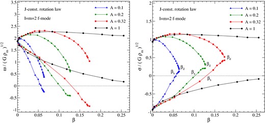
The l = m = 2 f mode frequency (left-hand panel) and the pattern speed (right-hand panel) with respect to the star's rotation β = T/|W| for four sequences of differentially rotating stars with, respectively, A = 0.1, 0.2, 0.32 and 1. The mode frequency and pattern speed are given in dimensionless units. The horizontal dotted line in each panel denotes the neutral line of the secular instability, β_s, where an initially retrograde mode (according to an inertial observer) becomes prograde as a result of star's rotation. The critical value β_d (indicated in the right-hand panel) denotes the points in the β–σ plane where the two branches of l = m = 2 f mode merge and, consequently, the dynamical bar-mode instability is expected to develop.

Nevertheless, the canonical energy and angular momentum provide important measures. In terms of the enthalpy, the canonical energy is given by (Friedman & Schutz 1978a)

\begin{eqnarray} E_{{\rm c}} &=& \frac{1}{2} \int {\rm d} \boldsymbol {r} \left[ \rho | \mathrm{\partial} _{t} \xi _{i} |^{2} - \rho | v^{j} \nabla _{j} \xi _{i} |^{2} + \rho \, \xi ^{i} \xi ^{j \ast } \nabla _{i} \nabla _{j} \left( h + \Phi \right) \right. \nonumber \\ && \left.+\, \frac{\mathrm{\partial} h}{\mathrm{\partial} \rho } \, | \delta \rho | ^2 - \frac{1}{4\pi G} | \nabla _{i} \delta \Phi | ^{2} \right], \end{eqnarray}

(25)

while the canonical angular momentum follows from (Friedman & Schutz 1978a)

\begin{equation} J_{{\rm c}} = - Re \int {\rm d} \boldsymbol {r} \rho \, \mathrm{\partial} _{\phi } \xi ^{i \ast } \left( \mathrm{\partial} _{t} \xi _{i} + v^{j} \nabla _{j} \xi _{i} \right), \end{equation}

(26)

where the integrals are calculated over the star's volume and Re denotes the real part. Note that these expressions are given in a coordinate basis, not the orthonormal basis used elsewhere in the paper. Building on the work of Saijo & Yoshida (2006) we will use the integrands from equations (25) and (26) to identify the region in the star where the instability develops.

3.1 The f mode

As we have already mentioned, the current understanding is that the low T/W instability sets in when the f mode enters the corotation region. In order to support this notion, it is natural to determine the mode frequencies along a differential rotation sequence and at the same time keep track of the corotation region. The latter task is straightforward since it only requires the background configurations. The determination of the oscillation frequencies for a set of stars along a given sequence is more time consuming. We obtain the required results by first evolving in time the linearized dynamical equations (11)–(13), and then calculating the mode frequencies by performing a fast Fourier transformation on the time evolution data. In order to test the reliability of the method we have confirmed that the results agree with data available in the literature (Karino, Yoshida & Eriguchi 2001; Karino 2003).

Fig. 1 shows the l = m = 2 f-mode frequencies, measured in the inertial reference frame, for four sequences of models with a different degree of differential rotation. The stars with the lowest level of differential rotation are parametrized by A = 1, while the highest differential rotation models have A = 0.1. For small values of A the fastest spinning stellar models assume a ‘toroidal-like configuration’ with a small axis ratio and a mass density whose maximum is not at the rotation axis. For instance, for A = 0.1 the fastest model studied in this work has β = 0.064 and R_p/R_eq = 0.067.

As expected, the results show that the f mode is rotationally split into two branches which are, respectively, prograde (m > 0) and retrograde (m < 0) with respect to the star's rotation. The prograde f-mode frequency gradually decreases for higher differential and more rapidly rotating models. Meanwhile, the retrograde f mode has an oscillation frequency which decreases with rotation and can become negative for rapidly rotating models. The neutral point, where the f-mode frequency is zero (indicated by β_s in Fig. 1), is important as it marks the point where an f mode is driven unstable by gravitational radiation via the well-known Chandrasekhar–Friedman–Schutz mechanism (Chandrasekhar 1970; Friedman & Schutz 1975, 1978a). This secular instability occurs when a locally retrograde mode is dragged forward by the star's rotation to the point where it is seen to be prograde by an inertial observer.

The conditions for the classical non-axisymmetric instabilities are better illustrated in the right-hand panel of Fig. 1, which shows the pattern speed, σ, for the l = m = 2 f mode against the rotation parameter β. The results in the figure can be compared to the results for incompressible ellipsoids (cf. fig. 5 in Andersson 2003). When a mode has a negative (positive) pattern speed, it is retrograde (prograde) with respect to the star. Note that in the notation used in this work, the azimuthal number m is taken negative for the retrograde mode. For the models shown in Fig. 1 with A ≤ 0.32, it is clear that the f mode is retrograde for slowly rotating stars, but becomes prograde at the critical rotation rate corresponding to β_s. Another significative point in the β–σ parameter space is where the pattern speeds of the two branches of the f mode merge. This point indicates where the classic dynamical bar-mode instability sets in in an inviscid star. Using our perturbative time evolutions we are able to extract the mode frequencies very close to this point, β_d, for the A = 0.1, 0.2 and 0.32 sequences.

The part of the parameter space where the low T/W instability might occur is shown in Fig. 2 for stellar models with A = 1 and in Fig. 3 for A = 0.32 and 0.1. For high differential rotation (small A), the corotation region increases considerably and the l = m = 2 f mode can enter this potential instability zone even for very slowly rotating stars. In Fig. 2, we also show the f-mode frequency calculated with the full perturbation problem, i.e. when the Poisson equation for the gravitational potential is solved alongside the fluid equations. It is well known that the Cowling approximation (where the gravitational potential perturbation is neglected) may introduce a significant error in the f-mode frequency (Karino 2003).

Figure 2.

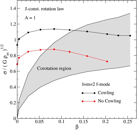
The pattern speed, σ = ω/m, of the l = m = 2 f mode is shown as a function of the rotation parameter β for differentially rotating stars with A = 1. The black (dots) and red (squares) show the values of σ from our simulations, respectively, in the Cowling and non-Cowling approximation case. The corotation band is represented by the grey region.

Figure 3.

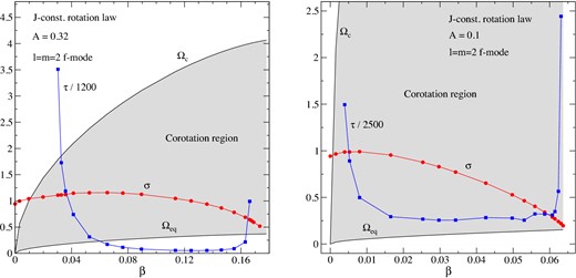
The inferred shear instability growth time, τ, for differentially rotating stars with A = 0.32 (left-hand panel) and A = 0.1 (right-hand panel). We also show the f-mode pattern speed, σ, and the corotation region (grey). All the quantities of this figure are shown in dimensionless units.

As we can see from Fig. 2, the f-mode frequencies are generally smaller when δΦ is included. In the present context, this is important since it affects the relation between the mode frequency and the corotation band. As indicated in the figure, the inclusion of the gravitational potential means that the instability may be triggered at lower rotation rates. Unfortunately, the solution of the Poisson equation (an elliptic equation), slows down the numerical simulations significantly which increases the time it would take to perform a large parameter space analysis. In addition, for differentially rotating models our code is more stable when the Cowling approximation is used. Since we do not expect the Cowling approximation to have any effect on the qualitative behaviour of the low T/W instability we will from now on focus on results obtained by neglecting δΦ.

3.2 Instability growth time

If the hypothesis from Watts et al. (2005) is correct, then the growth rate of the instability should depend on the position of the mode relative to the boundary of the corotation region, being more rapid deep inside the corotation region and essentially vanish at the corotation boundaries (as the mode stabilizes).

In order to assess this idea we determine the instability growth time-scale from our numerical simulations. As an example, we show in Fig. 4 the mode kinetic energy, E_k, for the rotating star models with A = 0.32. After some evolution time, the kinetic energy starts to grow exponentially with a rate that depends on the stellar rotation. We determine the instability growth time, τ, from a linear fit to the time evolved kinetic energy by assuming that

\begin{equation} E_k \sim {\rm e}^{ 2 \omega _I t }, \qquad \textrm {where} \qquad \omega _I = \frac{2 {\rm \pi }}{\tau }. \end{equation}

(27)

The kinetic energy is defined by the following equation:

\begin{equation} E_{k} = \frac{1}{2} \int {\rm d} \boldsymbol {r} \rho \, \delta \boldsymbol {{v}} ^{2}. \end{equation}

(28)

For this specific model, we find that the instability time-scale initially decreases as the rotation increases from a model with β = 0.04 up to a model with β = 0.136, and then increases again for more rapidly rotating configurations, i.e. β = 0.17. The rescaled growth times for the A = 0.32 and 0.1 cases are shown in Fig. 3, together with the pattern speed and the corotation region. The results clearly show that τ increases towards the boundaries of the corotation region. In fact, for models very close to these boundaries our time evolutions do not exhibit any instability. Most likely this is due to the numerical viscosity in the code preventing the instability from setting in until the physical growth overcomes the artificial damping. Real viscosity would, of course, play a similar role but it is orders of magnitude weaker than the numerical viscosity used in our simulations.

Figure 4.

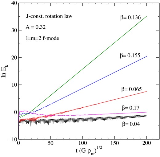
A sample of results for the time evolution of the kinetic energy associated with the f mode for models with A = 0.32 and different values for the rotation parameter β (see legend). The evolution time and the kinetic energy are given in dimensionless units. The vertical axis displays the natural logarithm of the kinetic energy, ln E_k.

In order to test the effect of the artificial viscosity on the inferred instability growth time we have considered several simulations with different numerical dissipation strength for a given stellar configuration. Thus, we found that τ is affected by the Kreiss–Oliger dissipation only at the level of about 0.1 per cent even when the viscosity factor is an order of magnitude larger than the fiducial one used, ϵ_D = 0.01. Hence, the extracted growth times are not significantly affected by the artificial damping. Of course, it is still the case that the numerical damping will overcome the growth of a very slowly growing unstable mode, e.g. near the corotation boundary.

In order to check that we are tracking a given unstable mode along the stellar sequence, we monitor the canonical energy and angular momentum integrands (see equations 25 and 26). Qualitatively, one would expect the unstable mode to be associated with the region near the corotation point in the star. If the low T/W instability is the result of an energy exchange between a corotating mode and the fluid bulk flow, this should be reflected in the energy and angular momentum integrands. This behaviour was, in fact, observed for the canonical angular momentum by Saijo & Yoshida (2006), who showed that the J_c integrand grows when an instability is present while remaining zero at the corotation point.

To study the behaviour of E_c and J_c it is useful to determine the cylindrical radius, ϖ_cor, at which a given mode corotates with the star (where ϖ = rsin θ). For the j-constant rotation law, we can determine from equation (21) and the mode frequency, ω, the following expression for the corotation point:

\begin{equation} \varpi _{{\rm cor}} = A \sqrt{ \frac{ m \Omega _c - Re\ \omega }{Re\ \omega } } \,. \end{equation}

(29)

In Fig. 5, we show the canonical energy distribution inside the star and the corotation radius ϖ_cor calculated from equation (29), for a selection of unstable models with A = 0.32. As expected, E_c grows around the corotation point and vanishes at ϖ_cor. The same feature has been observed for the canonical angular momentum. These results confirm that the growth time extracted from our numerical simulations is associated with the l = m = 2 f mode (as expected).

Figure 5.

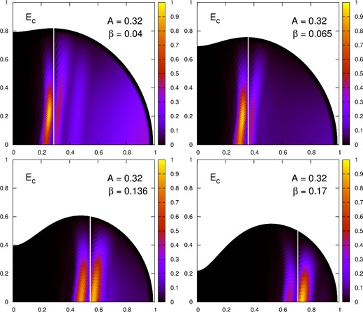
Examples of the extracted canonical energy density inside the neutron star. The vertical white line in each panel denotes the corotation cylindrical radius ϖ_cor.

The dependence of the instability growth time on the position of the corotation point is evident from Fig. 3. In order to understand the behaviour better, we consider the variation of τ with the degree of differential rotation and try to relate the results with the stellar parameters. Typical results are provided in Fig. 6, where we show the variation of the unstable mode's imaginary part, ω_I = 2π/τ, with respect to the rotation parameter β (left-hand panel) and cylindrical corotation radius (right-hand panel) for stars with A ranging between 0.1 and 0.6. Note that ϖ_cor = 0 corresponds to the condition σ = Ω_c, while ϖ_cor = 1 implies that σ = Ω_eq. Along each rotating sequence, corresponding to a specific A, ω_I exhibits a maximum inside the corotation band and decays towards the boundaries of the region. It is also interesting to note that for higher differential rotation the instability region appears at smaller rotation rates.

Figure 6.

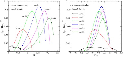
Imaginary part of the l = m = 2 mode frequency, ω_I = 2π/τ, for several sequences of differentially rotating stars with A = 0.1–0.6. The left- and right-hand panels show the dependence of ω_I, respectively, on the rotational parameter β and the cylindrical corotation radius ϖ_cor. The quantities on the horizontal and vertical axes are given in dimensionless units.

The results in Fig. 6 make qualitative sense given our expectations for the low T/W instability, but we would obviously like to understand the detailed features better. There are two main aspects to this. First of all, the maximum ω_I is not centred in the middle of the corotation band, where ϖ_cor = 0.5. Secondly, ω_I appears to reach its largest absolute value in the A = 0.4 model.

If the shear instability depends on an energy exchange between the bulk motion and the corotating mode, one would expect the instability time-scale to depend on the energy and degree of differential rotation present at the corotation point. Considering the behaviour of the variables involved, we find that the function,

\begin{equation} \psi = - \beta \left. \frac{\mathrm{\partial} \Omega }{\mathrm{\partial} \varpi } \right| _{\varpi _{{\rm cor}}}, \end{equation}

(30)

where the derivative of the star's angular velocity is calculated at the corotation radius, has a maximum at the same point as ω_I along the stellar sequence. Actually, we find that ψ increases from A = 0.1 to 0.5 and then decreases. Hence, the function ψ accounts reasonably well for the main features observed in our results, e.g. the faster instability growth of the model with A ∼ 0.4. Moreover, for each rotating model (with a given A) the function ψ can be used to determine the position of the shortest growth time inside the instability region.

It is worth noting that ψ can be re-written in terms of the star's parameters and the mode's pattern speed, using equation (29),

\begin{equation} \psi = \frac{ 2 \beta }{A \Omega _c } \left( \Omega _c - \sigma \right) ^{{1/2}} \sigma ^{{3/2}} \,. \end{equation}

(31)

Our numerical data suggest that ω_I is reasonably well approximated by the following empirical relation:

\begin{equation} \chi = a \, \psi ^{10 A} \,, \end{equation}

(32)

where a is a constant, and A is the usual differential rotation parameter. For the various models considered in this work the function χ is shown in Fig. 7, while the corresponding (dimensionless) values of a are given in Table 2. The maximum and the behaviour at small corotation radii are well captured by χ, there is a slight horizontal offset for A = 0.2 and 0.6 but they only amount to 1–2 per cent with respect to the ω_I peak. For larger ϖ_cor, the function χ generally assumes slightly larger values than ω_I, while for A = 0.1 the opposite is the case. For the latter model, this behaviour could be due to the presence of other unstable modes, but we did not manage to resolve this issue with our simulations.

Figure 7.

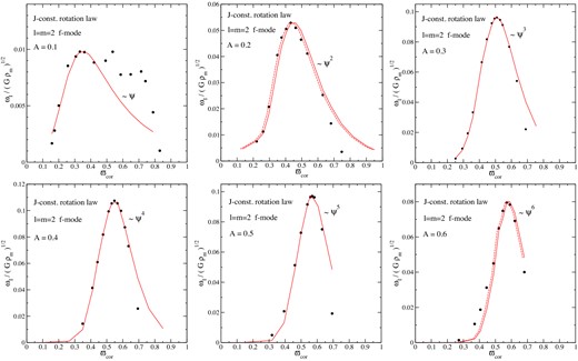
Comparison between the imaginary part of the l = m = 2 f mode and the empirical function χ for six differentially rotating models. Each panel corresponds to a model with a specific A (see legend). The horizontal and vertical axes show, respectively, the dimensionless ϖ_cor and ω_I. The filled dots represent the numerical values and the red lines the function χ. In the panels for the A = 0.2 and 0.6 models we also show a dashed red line, which provides a correction of the function χ to match the ω_I values.

Table 2.

The dimensionless values of the coefficient a, see equation (32), for stellar models with A = 0.1–0.6.

A	0.1	0.2	0.3	0.4	0.5	0.6
a	0.072	0.74	2.32	5.26	12.4	32.9

Table 2.

The dimensionless values of the coefficient a, see equation (32), for stellar models with A = 0.1–0.6.

A	0.1	0.2	0.3	0.4	0.5	0.6
a	0.072	0.74	2.32	5.26	12.4	32.9

Considering the explorative approach adopted in our investigation, it is interesting to note how well the function χ captures the main properties of the instability growth time and how it identifies the model with the strongest instability along a sequence. This provides interesting pointers towards future work. First of all, one should investigate if our empirical expression remains useful also for other models, e.g. different polytropic indices and rotational laws. If the suggestion proves robust one should also try to understand the underlying physics. This might shed useful light on the nature of this class of instabilities.

Before moving on, let us point out that most of the numerical results have been presented in dimensionless units, and the shortest growth time calculated in this work is |$\tau = 29.25 / \sqrt{G \rho _{\rm m} }$| for a model with A = 0.4 and axis ratio R_p/R_eq = 0.4. In physical units, this value is τ = 5.13 ms, for a typical star with M = 1.4M_⊙ and EoS parameters γ = 2 and k = 6.674 · 10⁴ g⁻¹cm⁵s⁻².

4 A SLIGHT ASIDE: THE INERTIAL R MODES

The perturbative time evolution code obviously allows us to consider a wider range of problems involving differentially rotating stars. As a pertinent example, let us make some comments on the inertial r modes. These modes are rotationally restored by the Coriolis force and are of particular interest since they suffer the gravitational-wave instability already at low rotation rates in uniform stars. Much effort has gone into understanding the astrophysical relevance of this instability, e.g. the role of various internal viscosity mechanisms, but the bulk of the work has considered stars in uniform rotation. If the r-mode instability acts very early on in a neutron star's life or is triggered in the hot remnant immediately after binary neutron star merger, then we would need to understand how differential rotation affects the mechanism. It is easy to see that the corotation point could be relevant for this discussion. According to an inertial observer the r mode is prograde for any stellar rotation rate with a frequency proportional to the bulk rotation rate (like all inertial modes). If such a mode enters the corotation region it should do so by crossing the low-frequency boundary which corresponds to the equatorial angular velocity Ω_eq (at least for ‘reasonable’ rotation laws like the j-constant law).

However, it is not clear from the results in the literature if the r mode actually enters the corotation region. So far, the r-mode frequency in differentially rotating stars has only been determined in Newtonian gravity by Karino et al. (2001). For a γ = 2 polytrope and the j-constant rotation law, their results show that the r mode is not in corotation for stars with A > 0.6. However, the mode clearly approaches the corotation band when A → 0.6. Unfortunately, the numerical code used by Karino et al. (2001) was not accurate for higher degrees of differential rotation (presumably because the corotation point corresponds to a singularity in the frequency domain description of the problem). As our numerical framework is based on time evolving the perturbation equations, our analysis is not affected by this issue and we can determine the r-mode frequency for lower values of A. This allows us to check if the r mode goes in corotation for a high degree of differential rotation. To carry out this exercise, we use the Cowling approximation which is known to provide accurate results for the r-mode frequency (Karino 2003). Considering models with a fixed axis ratio, r_ax = R_p/R_eq, respectively, r_ax = 0.95, 0.7 and 0.6, we determine the l = m = 2 r-mode frequency for A = 0.1–10. The results are shown in Fig. 8. We find that, even though the r mode approaches the corotation region as the degree of differential rotation is increased, it never really enters the corotation region (more than marginally). In all cases we have considered, the r mode stays very close to the equatorial boundary, i.e. ω ≃ mΩ_eq, as the rotation rate increases. We have found no evidence that the r mode suffers a shearing instability analogous to the low T/W instability in the f mode. It is not clear whether this is because no such instability exists or if it is simply the case that the growth time is too large to overcome the numerical dissipation in the examples we have studied (as one would expect for a mode located at the boundary of the corotation region).

Figure 8.

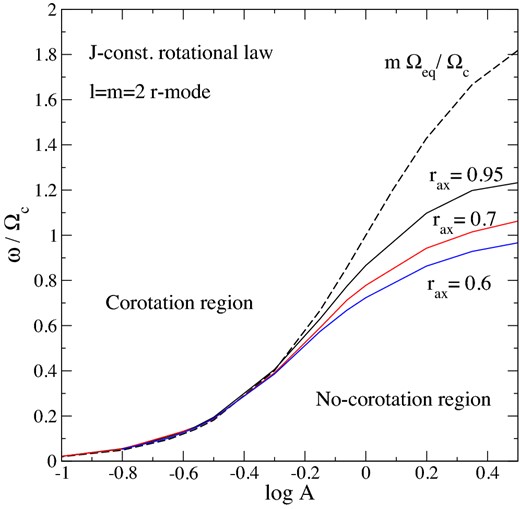
The dependence of the l = m = 2 r mode on the differential rotation parameter A, for three stellar configurations with a fixed axis ratio. They are, respectively, r_ax = 0.95, 0.7 and 0.6 (see legend). The dashed line denotes the equatorial boundary of the corotation region. The horizontal axis displays the quantity log A while the vertical axis gives the ratio between the mode frequency and the central angular velocity of the star. This figure can be directly compared to fig. 4 of Karino, Yoshida & Eriguchi (2001), where the numerical method became unreliable as the mode approached the corotation region.

5 CONCLUDING REMARKS

We have developed a framework for numerical time evolutions of linear perturbations of differentially rotating, Newtonian, stars. Within this framework, we have carried out a large parameter survey for polytropic stars described by the standard j-constant rotation law, focusing on the fundamental f mode and the low T/W instability. Our results for the instability growth time confirm the assertion of Watts et al. (2005) that the instability sets in at the point when the f mode first enters the corotation region (when there is a point in the star where the pattern speed in the star matches the local rotation rate of the background fluid). We have used the integrands of the canonical energy and angular momentum to highlight the close relationship between the instability and the corotation point. By considering the relevant stellar parameters we have also obtained a relatively simple empirical relation which describes how the growth rate of the low T/W instability increases as the f mode moves into the corotation region, reaches a maximum and then tapers off as the mode exits the unstable region again.

Our analysis has, in many ways, been of an exploratory nature. Our main aim was to map out the relevant parameter space and provide clear evidence for the link between the corotation boundary and the onset of instability. As they stand the results seem convincing in this respect. This is quite an important conclusion because it would be sufficient to know that the f mode of a given configuration lies inside the corotation region to know that the mode should be (at least in principle) unstable. Further work is needed to confirm this conclusion for other rotation laws and more realistic equations of state, but we have no reason to expect that the qualitative behaviour would change much in other cases. More detailed work is also needed in order to explain the form of the empirical relation we have found for the instability growth rate. Ideally, one would like to be able to derive this result from underlying principles, but this seems like a very difficult problem. One might be able to make progress using the canonical energy/angular momentum arguments from Friedman & Schutz (1975, 1978a,b). However, this would likely require a frequency domain approach which would be hampered by the singularity associated with the corotation point. Unfortunately, the fact that the instability analysis only holds (strictly) for inviscid systems means that we have been unable to use our results to make progress in this direction (the numerical simulations involve the standard artificial viscosity to stabilize the evolutions). We have also not been able to extract the mode eigenfunctions with sufficient precision due to the exponential growth of the perturbation variables during the instability. It seems possible that future work could do better in this regard. We would certainly encourage efforts in this direction.

Finally, we used our computational framework to consider the inertial r modes. In this case, our results extend previous work to higher degrees of differential rotation. We have demonstrated that the r modes do not (at least for our stellar models) evolve into the corotation region. Rather, they remain near the boundary of this region for rapidly and differentially rotating stars. This is an interesting result in its own right, and a clear demonstration of the usefulness of our numerical framework. The result may also be relevant for relativistic studies of the r mode where the frame dragging provides an effect that is qualitatively similar to differential rotation. For non-barotropic stars, in particular, the relativistic r-mode problem is known to be complicated. Based on the present evidence it would be tempting to suggest that time evolutions of the kind used in this work may prove a powerful tool also in that setting.

AP acknowledges support from the European Union Seventh Framework Programme (FP7/2007-2013) under grant agreement no. 267251 ‘Astronomy Fellowships in Italy (AstroFIt)’. NA acknowledges support from STFC in the UK and generous hospitality from the Institute for Nuclear Theory at the University of Washington where some of this work was carried out.

REFERENCES

Andersson

N.

,

Class. Quantum Grav.

,

2003

, vol.

20

pg.

105

Baiotti

L.

Pietri

R. D.

Manca

G. M.

Rezzolla

L.

,

Phys. Rev. D

,

2007

, vol.

75

pg.

044023

Camarda

K. D.

Anninos

P.

Fragile

P. C.

Font

J. A.

,

ApJ

,

2009

, vol.

707

pg.

1610

Centrella

J. M.

New

K. C. B.

Lowe

L. L.

Brown

J. D.

,

ApJ

,

2001

, vol.

550

pg.

L193

Cerdá-Durán

P.

Quilis

V.

Font

J. A.

,

Comput. Phys. Commun.

,

2007

, vol.

177

pg.

288

Chandrasekhar

S.

,

Ellipsoidal Figures of Equilibrium

,

1969

New Haven, CT

Yale Univ. Press

Google Scholar

Google Preview

OpenURL Placeholder Text

WorldCat

Chandrasekhar

S.

,

Phys. Rev. Lett.

,

1970

, vol.

24

pg.

611

Corvino

G.

Rezzolla

L.

Bernuzzi

S.

De Pietri

R.

Giacomazzo

B.

,

Class. Quantum Grav.

,

2010

, vol.

27

pg.

114104

Franci

L.

De Pietri

R.

Dionysopoulou

K.

Rezzolla

L.

,

Phys. Rev. D

,

2013

, vol.

88

pg.

104028

Friedman

J. L.

Schutz

B. F.

,

ApJ

,

1975

, vol.

200

pg.

204

Friedman

J. L.

Schutz

B. F.

,

ApJ

,

1978a

, vol.

221

pg.

937

Friedman

J. L.

Schutz

B. F.

,

ApJ

,

1978b

, vol.

222

pg.

281

Fu

W.

Lai

D.

,

MNRAS

,

2011

, vol.

413

pg.

2207

Hachisu

I.

,

ApJS

,

1986

, vol.

61

pg.

479

Jones

D. I.

Andersson

N.

Stergioulas

N.

,

MNRAS

,

2002

, vol.

334

pg.

933

Karino

S.

,

MNRAS

,

2003

, vol.

343

pg.

175

Karino

S.

Yoshida

S.

Eriguchi

Y.

,

Phys. Rev. D

,

2001

, vol.

64

pg.

024003

Kuroda

T.

Umeda

H.

,

ApJS

,

2010

, vol.

191

pg.

439

Muhlberger

C. D.

et al. ,

2014

preprint (arXiv:1405.2144)

Ott

C. D.

Ou

S.

Tohline

J. E.

Burrows

A.

,

ApJ

,

2005

, vol.

625

pg.

L119

Ott

C. D.

Dimmelmeier

H.

Marek

A.

Janka

H.-T.

Hawke

I.

Zink

B.

Schnetter

E.

,

Phys. Rev. Lett.

,

2007

, vol.

98

pg.

261101

PubMed

Ou

S.

Tohline

J. E.

,

ApJ

,

2006

, vol.

651

pg.

1068

Papaloizou

J. C.

Pringle

J. E.

,

MNRAS

,

1980

, vol.

190

pg.

43

Papaloizou

J. C. B.

Pringle

J. E.

,

MNRAS

,

1984

, vol.

208

pg.

721

Passamonti

A.

Haskell

B.

Andersson

N.

Jones

D. I.

Hawke

I.

,

MNRAS

,

2009a

, vol.

394

pg.

730

Passamonti

A.

Haskell

B.

Andersson

N.

,

MNRAS

,

2009b

, vol.

396

pg.

951

Saijo

M.

Yoshida

S.

,

MNRAS

,

2006

, vol.

368

pg.

1429

Saijo

M.

Baumgarte

T. W.

Shapiro

S. L.

,

ApJ

,

2003

, vol.

595

pg.

352

Scheidegger

S.

Fischer

T.

Whitehouse

S. C.

Liebendörfer

M.

,

A&A

,

2008

, vol.

490

pg.

231

Schutz

B. F.

,

MNRAS

,

1980a

, vol.

190

pg.

7

Schutz

B. F.

,

MNRAS

,

1980b

, vol.

190

pg.

21

Shibata

M.

Baumgarte

T. W.

Shapiro

S. L.

,

ApJ

,

2000

, vol.

542

pg.

453

Shibata

M.

Karino

S.

Eriguchi

Y.

,

MNRAS

,

2002

, vol.

334

pg.

L27

Shibata

M.

Karino

S.

Eriguchi

Y.

,

MNRAS

,

2003

, vol.

343

pg.

619

Watts

A. L.

Andersson

N.

Jones

D. I.

,

ApJ

,

2005

, vol.

618

pg.

L37