


Abstract
We report the serendipitous detection of a 0.2 L*, Lyα emitting galaxy at redshift 2.5 at an impact parameter of 50 kpc from a bright background QSO sightline. A high-resolution spectrum of the QSO reveals a partial Lyman-limit absorption system (|${\it N}_\mathrm{H\,\small {i}}=10^{16.94\pm 0.10}$| cm−2) with many associated metal absorption lines at the same redshift as the foreground galaxy. Using photoionization models that carefully treat measurement errors and marginalize over uncertainties in the shape and normalization of the ionizing radiation spectrum, we derive the total hydrogen column density |${\it N}_\mathrm{H}=10^{19.4\pm 0.3}\,\rm cm^{-2}$|, and show that all the absorbing clouds are metal enriched, with Z = 0.1–0.6 Z⊙. These metallicities and the system's large velocity width (436 km s− 1) suggest the gas is produced by an outflowing wind. Using an expanding shell model we estimate a mass outflow rate of ∼5 M⊙ yr−1. Our photoionization model yields extremely small sizes (<100–500 pc) for the absorbing clouds, which we argue is typical of high column density absorbers in the circumgalactic medium (CGM). Given these small sizes and extreme kinematics, it is unclear how the clumps survive in the CGM without being destroyed by hydrodynamic instabilities. The small cloud sizes imply that even state-of-the-art cosmological simulations require more than a 1000-fold improvement in mass resolution to resolve the hydrodynamics relevant for cool gas in the CGM.
1 INTRODUCTION
Observations of the gaseous haloes surrounding galaxies – the circumgalactic medium (CGM) – allow us to constrain two of the most poorly understood aspects of galaxy formation: galactic-scale winds and gas accretion on to galaxies. Detecting this gas in emission at high redshift is possible, but only in extreme environments or with very deep observations (e.g. Steidel et al. 2011; Rauch et al. 2013; Cantalupo et al. 2014; Martin et al. 2014) using current facilities. The diffuse gas comprising galactic-scale winds and accreting gas can be relatively easily measured as rest-frame UV absorption features, however, which are imprinted on the spectrum of the galaxy itself (‘down the barrel’), or on a background QSO at a small impact parameter from the galaxy.
Observations of blueshifted absorption in galaxy spectra have shown that galactic-scale winds are common from z ∼ 0.5 (Weiner et al. 2009; Martin et al. 2012; Rubin et al. 2013) to z ∼ 3 (Pettini et al. 2001; Adelberger et al. 2005; Steidel et al. 2010; Bielby et al. 2011). In some cases redshifted absorption is also seen, suggesting the presence of metal-enriched, inflowing gas (Martin et al. 2012; Rubin et al. 2012). However, the faintness of the background galaxies used by these studies mean that only low-resolution spectra can be used, and the absorption lines are not resolved. Therefore the metallicity, ionization state, and volume density of the gas remain poorly determined. Background QSOs are much brighter than galaxies, and thus a high-resolution spectrum of a QSO at small impact parameter (≲100 kpc) from a foreground galaxy can resolve individual metal transitions in the galaxy's CGM. Precise column density measurements then enable us to tightly constrain the physical properties of the gas using photoionization models.
A growing sample of QSO absorber–galaxy pairs is being assembled by searching for galaxies around strong z ∼ 3 damped-Lyα (DLA) systems |${\it N}_\mathrm{H\,\small {i}}> 10^{20.3}\,{\rm cm^{-2}}$| (e.g. Djorgovski et al. 1996; Møller et al. 2002; Péroux et al. 2011; Fynbo et al. 2013). This technique has found one example that may be caused by accreting gas (Bouché et al. 2013) and others that may be produced by outflowing gas (e.g. Noterdaeme et al. 2012; Krogager et al. 2013; Péroux et al. 2013). However, a drawback of this approach is that by construction, these pairs only represent the strongest, often metal-rich absorbers. In addition, the physical properties of individual absorbing components cannot be measured, as line saturation and the Lyα damping wings make it difficult to divide the total observed |${\it N}_\mathrm{H\,\small {i}}$| between different metal components.
An alternative approach is to search for galaxies close to QSO sightlines without any absorption pre-selection. This allows a census of gas around galaxies for a wide range of absorption properties. Several surveys have been undertaken to assemble such samples (Adelberger et al. 2003, 2005; Crighton et al. 2011; Rudie et al. 2012). Simcoe et al. (2006) performed the first photoionization modelling of a ‘partial’ Lyman-limit system (LLS)1 with |${\it N}_\mathrm{H\,\small {i}}\approx 10^{16}$| cm−2 at an impact parameter of 115 kpc from a z = 2.3 galaxy found by one of these surveys. The absorption they see can be explained by small, ∼100 pc scale, metal-enriched gas clumps suggestive of an outflowing wind. Recently Crighton, Hennawi & Prochaska (2013b) analysed a different galaxy–absorber pair at z = 2.4 with an impact parameter of 55 kpc. They detected low-metallicity gas with properties consistent with those expected for ‘cold-mode’ accretion. They also detect metal-enriched gas in the same absorber. However, they found that the inferred metallicity of the higher-Z gas depends strongly on the shape assumed for the ionizing spectrum used when modelling the clouds.
In this work we report the discovery of a partial LLS with |${\it N}_\mathrm{H\,\small {i}}= 10^{16.9}\,\rm cm^{-2}$| caused by metal-enriched gas that is coincident in redshift with a Lyα-emitting galaxy (LAE), fainter than those selected with the traditional Lyman-break techniques. The absorber is at an impact parameter ρ = 50 kpc from the galaxy. We use a new modelling procedure which marginalizes over uncertainties in the ionizing radiation spectrum to make robust measurements of the metallicity and volume density of the gas.
Our paper is structured as follows. In Section 2 we describe the galaxy properties. Section 3 describes the properties of the partial LLS, and how we perform cloudy modelling to derive the metallicity and density of the absorbing gas. Section 4 considers different scenarios that reproduce our observations and discusses implications for simulations of the CGM. Section 5 discusses the implications of our results for simulations of the CGM. Section 6 summarizes our results. The appendices give details about our photoionization modelling method. We use a Planck 2013 cosmology (ΩM = 0.31, |$\Omega _\Lambda =0.69$|, H0 = 68 km s− 1 Mpc− 1; Planck Collaboration XVI 2013), and all distances listed are proper (not comoving) unless stated otherwise.
2 THE Lyα-EMITTING FAINT GALAXY AT z = 2.466
The galaxy was serendipitously discovered in a survey for z ∼ 2.5 galaxies around QSO sightlines (Cooksey et al., in preparation; Crighton et al., in preparation). The original aim of these observations was to confirm galaxy candidates with r′ magnitude <25.5 around the sightline to the QSO Q0002−422 (RA 00h04m48.1s, Dec. −41°57′29′′ [J2000] zQSO = 2.76, r = 17.4). This QSO was selected without reference to any absorption in the spectrum (i.e. the presence of a DLA or LLS). The galaxy we analyse in this paper is too faint to satisfy the r′ < 25.5 selection criterion, but happened to fall inside a slit targeting a brighter object near the QSO. It was detected by its Lyα emission line, which we then linked to a faint continuum source in deep imaging of the field. Fig. 1 shows a false colour image generated from this deep imaging in the u′, g′ and r′ bands. This imaging was taken with the MagIC CCD camera on the Magellan Clay telescope in 2005 October, with total exposure times of 1.5 h each in g′ and r′ and 5 h in u′. The images were bias-subtracted, flat-fielded, registered and combined using standard iraf procedures and smoothed to a common seeing scale of 0.6 arcsec (set by u′) to facilitate measurement of isophotal colours. The 5σ detection limits for a point source in the combined images are 26.3 (u′), 27.7 (g′) and 28.0 (r′).
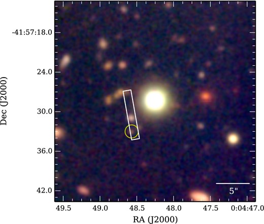
u′, g′ and r′ composite from Magellan/MagIC imaging showing the QSO (centre) and the nearby slit where Lyα emission is seen at z = 2.466. The circled object is the r = 25.9 continuum source we associate with the Lyα line. It is offset 3.53 arcsec east and 4.68 arcsec south of the QSO, corresponding to an impact parameter of 49 proper kpc at z = 2.466. The object at the centre of the slit is an unrelated galaxy at z < 2.
The QSO is shown at the centre of Fig. 1, and the slit in which the emitter falls is on left. The brighter object at the centre of this slit was the galaxy candidate originally targeted. Its redshift is uncertain, but the absence of Lyα forest absorption requires z < 2. We identify the fainter, circled object as the continuum source associated with the emitter. SExtractor was used to measure magnitudes for this source in a 1.5 arcsec aperture, giving u = 26.8 ± 0.2, g = 26.08 ± 0.08 and r = 25.90 ± 0.08 (AB). Its colours satisfy the BX selection criteria, designed to select star-forming galaxies in the redshift range 2.0 < z < 2.5 (Steidel et al. 2004) based on their continuum emission.
We obtained the galaxy spectrum during programme 091.A-0698 (PI: Crighton) using FORS2 at the Very Large Telescope (VLT) with the 600B+22 grism and a 1.2 arcsec slit, resulting in a resolution of 650 ( ∼ 460 km s− 1). A total of five 30 min exposures were taken over 2013 September 8 and 9 in clear conditions with seeing 0.8–1 arcsec. The exposures were flat-fielded, combined and wavelength-calibrated using Low Redux.2 Observations of a standard star were used to flux calibrate the 1D spectrum, which covers a wavelength range 3600–6000 Å. The Lyα line that revealed the galaxy is shown in Fig. 2. It is offset from the trace of the brighter, original target seen in the centre of the top panel. By fitting a Gaussian to the line, we measure an emission redshift |$z_\mathrm{\rm Ly\alpha }=2.4659\pm 0.0003$|. The line is not resolved in this spectrum, so must have an intrinsic full width at half-maximum significantly less than 460 km s− 1. The FORS spectral resolution is not high enough to separate the [O ii] doublet (λ3727, λ3729), which has a separation of 220 km s− 1. However, there are no other emission lines detected in the spectrum. This means that the line is unlikely to be caused by [O ii] at z = 0.13, because then we would also expect to detect H-β (λ4863) and [O iii] (λ3727, λ3729). The line width is much narrower than expected for broad lines from a QSO, and no C iv emission at z = 2.4659 is detected. Therefore the emission is unlikely to be caused by an active galactic nucleus (AGN). Lyα is typically offset bluewards from the systemic redshift in brighter Lyman-break selected galaxies by 300 ± 125 km s− 1 (Rakic et al. 2011). For the small sample of fainter LAEs where Hα has been measured in addition to Lyα, a smaller blue offset of 220 ± 30 km s− 1 is found (Yang et al. 2011; Hashimoto et al. 2013a,b). Therefore we adopt an intrinsic redshift |$z_\mathrm{gal} = z_\mathrm{\rm Ly\alpha } - (220\,\mathrm{\rm km\,s^{-1}}/c)(1+z_\mathrm{\rm Ly\alpha }) = 2.4636$| with an uncertainty of 125 km s− 1.
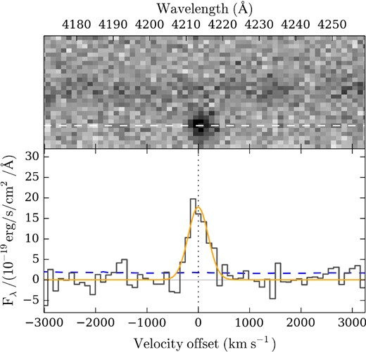
FORS spectrum showing the Lyα emission line. The top panel shows the emission line, offset from the trace of the central object that was the original target (which has z < 2). A dashed white line shows the assumed trace used to extract the emission line. The bottom panel shows the extracted 1D spectrum with the 1σ error array (blue dashed line), and a Gaussian profile fitted to the line, assuming a width given by the spectral resolution. The line is unresolved, implying an intrinsic width significantly less than 460 km s− 1, corresponding to the FORS spectral resolving power of 650. The velocity scale is relative to z = 2.466.
2.1 The measured star formation rate
The Lyα line flux is 1.1 × 10⁻¹⁷ erg s−1 cm−2, which implies a lower limit to the star formation rate SFRLyα > 0.5 M⊙ yr−1 assuming case B recombination (Draine 2011, section 14.2.3) and no dust extinction. The rest-frame UV continuum gives an independent measure of the SFR. Using the mean of the g′- and r′-band magnitude to estimate the rest-frame UV continuum magnitude M1700, then applying a UV-to-SFR conversion factor of 7.2 × 10⁻¹⁹ (appropriate for a Kroupa IMF and log10[Z/Z⊙] = −0.5, Madau & Dickinson 2014) results in a SFRUV ≈ 1.5 M⊙ yr−1. This is a factor of 3 larger than SFRLyα. This discrepancy can easily be explained by slit losses, which we expect to be large as the was not centred on the slit, or preferential scattering or dust absorption of Lyα photons with respect to the continuum emission. The rest-frame UV luminosity corresponds to 0.2L*, using |$M_{1700}^*=-21.0$| (Reddy & Steidel 2009).
Would this galaxy be classified as an LAE, as studied by narrow band surveys (Gawiser et al. 2007; Nilsson et al. 2011)? LAEs are empirically classified as satisfying rest equivalent width (Wr ≳ 20 Å in the rest frame) and line flux criteria (≳1 × 10⁻¹⁷ erg s−1 cm−2). No continuum is detected in the FORS spectrum, and conservatively adopting the 1σ error level as an upper limit to the continuum gives a lower limit Wr > 15 Å. We can also estimate the continuum flux using the g-band magnitude (the emission line does not make a significant contribution to this band), which yields Wr > 16 Å. This is also a lower limit as slit losses could be significant. We conclude from the Lyα line strength and equivalent width lower limits that this object would indeed be selected as an LAE.
2.2 Galaxy mass and SED fitting
Currently only rest-frame UV magnitudes are available for the galaxy, which makes it difficult to measure a stellar mass via spectral energy distribution (SED) modelling. However, the faint UV magnitudes suggest a smaller stellar mass than is typical of BX-selected galaxies. Fig. 3 shows the distribution of r − g colours and stellar masses in the Hubble Ultra Deep Field (UDF) for galaxies with a similar r magnitude and redshift to the galaxy in this work (from the SED fitting performed by da Cunha et al. 2013). The median stellar mass of these objects is 109.14 M⊙, with 16th and 84th percentiles of 108.8 and 109.4 M⊙. This range is significantly smaller than the typical stellar mass of BX-selected galaxies with R < 25.5, 1010.32 ± 0.51 M⊙ (Shapley et al. 2005). Moreover, we demonstrated in the previous section that this galaxy would be classified as an LAE. Clustering analyses show that LAEs have a typical halo mass |$\log _{10}({\rm M}/\,{\rm M}_{\odot })=10.9^{+0.5}_{-0.9}$| (Gawiser et al. 2007), smaller than that of BX-selected galaxies (M/ M⊙ = 1011.5−12.0, Adelberger 2005; Conroy et al. 2008; Bielby et al. 2013). This lower halo mass is consistent with the value found by converting a stellar mass of 109.14 M⊙ to a halo mass using the relation from Moster, Naab & White (2013): 1011.4 M⊙.
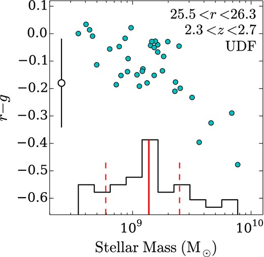
r − g colours as a function of stellar mass for galaxies in the Hubble Ultra Deep Field with a similar redshift (2.3 < z < 2.7) and magnitude (25.5 < r < 26.3) to the galaxy in this work. Stellar masses are taken from da Cunha et al. (2013). The open circle shows r − g and its 1σ uncertainty for our z = 2.5 galaxy (its x-axis position is arbitrary). The 16th, 50th (median) and 84th percentiles of the stellar mass are 108.8, 109.1 and 109.4 M⊙, shown by red vertical lines. This stellar mass range is lower than that of brighter BX-selected galaxies (M* ∼ 2 × 10¹⁰ M⊙; Shapley et al. 2005).
Keeping the limitations of SED modelling in mind, we used the measured u′, g′ and r′ colours to estimate the galaxy's stellar mass with the SED fitting code magphys (da Cunha, Charlot & Elbaz 2008). We corrected for H i absorption from the intergalactic medium (IGM) in the u′ and g′ bands using IGMtransmission3 (Harrison, Meiksin & Stock 2011), which calculates the mean absorption using the transmission curves of Meiksin (2006). The inferred stellar mass (16th, 50th and 84th percentiles of 108.8, 109.4 and 109.7 M⊙) is consistent with the range given above for UDF galaxies with a similar magnitude and redshift. These models also predict a low SFR, similar to that estimated from the rest-frame UV magnitude, and little dust extinction. A low dust extinction is consistent with the low extinction measured for LAEs, E(B − V) < 0.02 (Gawiser et al. 2007).
We conclude that it is likely that the galaxy has a stellar mass of ∼109.1 M⊙ (corresponding to a specific SFR ∼1.1 Gyr−1) and halo mass of ∼1011.4 M⊙. We adopt a fiducial halo mass of 1011.4 M⊙, which corresponds to a virial radius of 60 kpc, and indicate where our conclusions would change assuming a higher halo mass. Deep rest-frame optical and near-IR imaging are required for a more precise measurement of the galaxy's stellar mass.
3 THE NEARBY PARTIAL LYMAN-LIMIT SYSTEM
Quasar Q0002−422, initially identified by its strong Lyα emission in a prism survey (Osmer & Smith 1976), has been extensively observed with the Ultraviolet and Visual Echelle Spectrograph (UVES) on the VLT in Chile. We retrieved 49.5 h of exposures from the European Southern Observatory (ESO) data archive, spread over 43 individual exposures ranging between 3600 and 6500 s in duration each. These were observed under two different programmes, 166.A-0106 (PI: Bergeron) and 185.A-0745 (PI: Molaro),4 over 2001 July–2002 September and 2010 October–2012 November, during which the prevailing observing conditions varied substantially, delivering seeing of 0.5–1.5 and 0.6–1.3 arcsec, respectively. The slit widths varied between the two programmes (1.0 and 0.8 arcsec, respectively), so the spectral resolutions obtained in the individual exposures varied between ∼45 000 and ∼60 000.
The ESO UVES Common Pipeline Language data reduction software was used to optimally extract and calibrate the relative quasar flux and wavelength scales, and uves_popler5 was used to combine the many exposures into a single, normalized spectrum on a vacuum-heliocentric wavelength scale. The 43 exposures were taken with a wide variety of UVES wavelength settings which, when combined, cover 3050 to 9760 Å. The final signal-to-noise ratio (S/N) is 25 per 2 km s− 1 pixel at 3200 Å and >70 pix−1 between 4100 and 9200 Å.
It is desirable to combine all of the available exposures to maximize the S/N. However, if the transitions we measure are unresolved by the lower resolution R ∼ 45 000 spectra, then using a combination of the higher and lower resolution spectra could bias the derived absorber parameters. Therefore we checked that relevant transitions are resolved by the lower resolution exposures by making two combined spectra, one from each subset of exposures with a common slit width. There was no change in the absorption profiles of interest between these two spectra, which indicates that the profiles are indeed resolved by the lower resolution. We thus use a single combined spectrum from all the exposures for our analysis.
3.1 Measurement of column densities
The QSO spectrum reveals a partial LLS (|${\it N}_\mathrm{H\,\small {i}}=10^{16.94\pm 0.10}$| cm−2) at z = 2.4639, ∼ 150 km s− 1 bluewards of the galaxy's Lyα emission redshift. C ii, C iii, C iv, Si ii, Si iii, Si iv, Mg ii, Fe iii, Al ii, Al iii and O vi transitions are present, and there are eight clearly separable absorption components that cover a velocity range of 436 km s− 1 (see Fig. 4). A single velocity structure can adequately fit all the low ions (which we define as having an ionization potential <3 Ryd).6 O vi roughly follows the velocity structure of the lower ions, but its components are not always precisely aligned with the lower ionization potential ions, and the widths are much larger than would be expected if they were produced by the same gas as the low ions. Si iv and C iv show a mixture of both broad components aligned with O vi, and narrower components aligned with the low ions. We discuss the origin of the O vi absorption in Section 4.5.
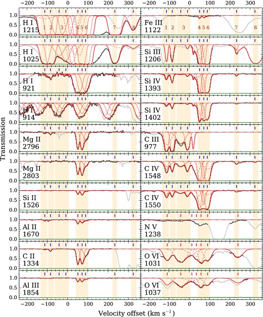
Neutral hydrogen and metal transitions in the partial LLS associated with the emitter. Zero velocity is at z = 2.4633. This is − 220 km s− 1 from the redshift of the galaxy Lyα emission line, which is a typical Lyα offset from the intrinsic redshift for LAEs. The thick red curve shows the model we fit to the UVES spectrum (dark histogram), and the thin green line near zero is the 1σ uncertainty in the transmission. The greyed out regions are blended with unrelated absorption. The thin red solid curves show the individual components we use in our cloudy modelling, and dotted curves are other components we do not model. The component numbers from Tables 1 and 2 are shown in the top panels (note that component 3 is made up of two subcomponents, shown by the 3rd and 4th ticks from the left). Metal transitions are seen over a velocity width of 436 km s− 1, and a single velocity structure, shown by blue ticks, can explain H i and all the low-ion metal transitions. Different components are needed to fit O vi; these are shown by red ticks in the bottom-right panels. We applied a −1.2 km s− 1 offset (0.6 pixels) to the Si iii absorbing region. The origin of this shift is unclear, but it may be caused by wavelength calibration uncertainties. N v λ1242 is blended with forest absorption, and so we use N v λ1238 to give an upper limit on NNV.
Due to the high S/N and coverage of the Lyman limit (Fig. 5), |${\it N}_\mathrm{H\,\small {i}}$| can be precisely measured in each low-ion component, enabling us to place tight constraints on the metallicity and other physical conditions of the gas using photoionization modelling. We measured column densities by fitting Voigt profiles with VPFIT;7 parameters are given for each component in Table 1.
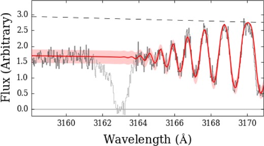
The Lyman limit of the z = 2.466 absorber. The solid curve and range shows a single component model with |${\it N}_\mathrm{H\,\small {i}}=10^{16.94\pm 0.10}\,\rm cm^{-2}$|, where the uncertainty includes a 5 per cent error in the continuum level. The dashed line shows our adopted continuum level and the greyed out region is unrelated absorption.
The redshift, b parameter, column density and their 1σ uncertainties for the eight components shown in Fig. 4. Upper limits are calculated using the 5σ equivalent width detection limit for undetected transitions, and by measuring the highest column density Voigt profile consistent with the data for blended transitions.
| Ion | z | b(km s− 1) | log 10N(cm− 2) | Ion | z | b(km s− 1) | log 10N(cm− 2) | |
|---|---|---|---|---|---|---|---|---|
| Component 1 (velocity = −112 km s− 1) | Component 5 (velocity = 72 km s− 1) | |||||||
| H i | 2.462 033(02) | 17.4 ± 0.1 | 14.88 ± 0.01 | H i | 2.464 158(01) | 17.0c | 16.5 ± 0.1 | |
| O i | <12.41 | O i | <12.77 | |||||
| Mg ii | 5.6a | 11.4 ± 0.2 | Mg ii | 7.0d | 12.91 ± 0.01 | |||
| Si ii | <11.77 | Si ii | 6.75d | 12.85 ± 0.01 | ||||
| Si iii | <12.8 | Si iii | 6.8d | >13.75 | ||||
| Si iv | 5.5 ± 1.0a | 12.22 ± 0.03 | Si iv | 6.8d | 13.43 ± 0.01 | |||
| C ii | 7.1a | 12.22 ± 0.14 | C ii | 8.6 ± 0.2d | 13.72 ± 0.01 | |||
| C iii | >13.0 | C iii | 6.8d | – | ||||
| C iv | 7.1a | 13.06 ± 0.02 | C iv | 13.74 ± 0.04 | ||||
| Al ii | 5.5a | 11.1 ± 0.2 | Al ii | 8.6d | 11.528 ± 0.036 | |||
| Al iii | 5.5a | 10.8 ± 0.4 | Al iii | 6.6d | 12.025 ± 0.017 | |||
| Fe iii | <13.0 | Fe iii | 6.0d | 12.97 ± 0.05 | ||||
| N ii | <13.28 | N ii | <13.18 | |||||
| N v | <12.8 | N v | <13.6 | |||||
| O vi | <14.0 | O vi | <14.0 | |||||
| Component 2 (velocity = −84 km s− 1) | Component 6 (velocity = 92 km s− 1) | |||||||
| H i | 2.462 361(01) | 14.2 ± 0.3 | 15.232 ± 0.012 | H i | 2.464 358(01) | 17.0c | 16.2 ± 0.15 | |
| O i | <12.4 | O i | <12.77 | |||||
| Mg ii | 5.3a | 11.52 ± 0.09 | Mg ii | 11.5e | 12.476 ± 0.017 | |||
| Si ii | <11.83 | Si ii | 11.5e | 12.343 ± 0.016 | ||||
| Si iii | <12.9 | Si iii | >13.5 | |||||
| Si iv | 5.5a | 12.593 ± 0.009 | Si iv | 11.5 ± 0.1e | 13.675 ± 0.005 | |||
| C ii | 6.4 ± 0.9a | 12.56 ± 0.04 | C ii | 11.5e | 13.37 ± 0.01 | |||
| C iii | >13.2 | C iii | – | |||||
| C iv | 6.4a | 13.097 ± 0.009 | C iv | 11.5e | 14.189 ± 0.015 | |||
| Al ii | 5.2a | 10.64 ± 0.25 | Al ii | 11.5e | 11.27 ± 0.08 | |||
| Al iii | 5.2a | 10.94 ± 0.18 | Al iii | 11.5e | 11.794 ± 0.034 | |||
| Fe iii | <12.5 | Fe iii | 11.5e | 12.84 ± 0.09 | ||||
| N ii | <12.2 | N ii | <13.18 | |||||
| N v | <12.8 | N v | <13.6 | |||||
| O vi | <14.0 | O vi | <14.0 | |||||
| Component 3 (velocity = −45 to − 5 km s− 1) | Component 7 (velocity = 235 km s− 1) | |||||||
| H i | 2.462 848(04), | 14.6 ± 0.3 | H i | 2.466 027(04) | 19.1 ± 0.4 | 14.70 ± 0.01 | ||
| O i | 2.463 234(02)b | <12.59 | O i | <13.18 | ||||
| Mg ii | <11.71 | Mg ii | <11.40 | |||||
| Si ii | <11.97 | Si ii | <11.39 | |||||
| Si iv | |$12.28_{-0.11}^{+0.25}$| | Si iii | <12.1 | |||||
| C ii | <12.06 | Si iv | 5.7 ± 0.9 | 11.88 ± 0.04 | ||||
| C iii | 13.65 ± 0.3 | C ii | <12.36 | |||||
| C iv | |$13.52_{-0.08}^{+0.15}$| | C iv | 8 ± 1 | 12.53 ± 0.04 | ||||
| Al ii | <11.02 | Al ii | <10.84 | |||||
| Al iii | <11.19 | Al iii | <11.11 | |||||
| Fe iii | <12.7 | Fe iii | <14.50 | |||||
| N ii | <12.47 | N ii | <12.65 | |||||
| N v | <12.75 | N v | <13.1 | |||||
| O vi | <14.0 | O vi | <14.0 | |||||
| Component 4 (velocity = 51 km s− 1) | Component 8 (velocity = 324 km s− 1) | |||||||
| H i | 2.463 919(01) | 17.00c | 16.5 ± 0.1 | H i | 2.467 073(13) | 21.1 ± 0.3 | 13.59 ± 0.01 | |
| O i | <12.77 | O i | <12.42 | |||||
| Mg ii | 5.7a | 12.824 ± 0.013 | Mg ii | <11.60 | ||||
| Si ii | 5.5a | 12.68 ± 0.02 | Si ii | <11.74 | ||||
| Si iii | >13.5 | Si iii | – | |||||
| Si iv | 5.5a | 13.630 ± 0.016 | Si iv | <11.19 | ||||
| C ii | 7.0 ± 0.1a | 13.69 ± 0.01 | C ii | – | ||||
| C iv | 7.0a | 14.076 ± 0.031 | C iv | 6.7 ± 2 | 12.01 ± 0.08 | |||
| Al ii | 5.5a | 11.59 ± 0.03 | Al ii | <10.82 | ||||
| Al iii | 5.5a | 12.00 ± 0.02 | Al iii | <11.10 | ||||
| Fe iii | 4.8a | 13.08 ± 0.04 | Fe iii | <13.7 | ||||
| N ii | <13.18 | N ii | – | |||||
| N v | <13.6 | N v | <13.7 | |||||
| O vi | <14.0 | O vi | <14.0 | |||||
Notes:ab value is tied for all metal species assuming turbulent broadening bturb = 4 km s− 1.
bThis component is made up of two subcomponents with the listed redshifts. Column densities are for the sum of both subcomponents.
cb value fixed.
db value is tied for all metal species assuming turbulent broadening bturb = 5 km s− 1.
eb value is tied for all metal species assuming purely turbulent broadening.
3.2 Photoionization modelling
Following previous analyses (e.g. D'Odorico, Dessauges-Zavadsky & Molaro 2001; Fox et al. 2005; Simcoe et al. 2006; Prochaska & Hennawi 2009; Fumagalli, O'Meara & Prochaska 2011a; Crighton et al. 2013b), we use the observed column densities to infer a metallicity and volume density for each component by comparison to cloudy photoionization model predictions. However, in contrast to these previous analyses we add another free parameter to represent uncertainty in the shape of the UV ionizing background. It has been shown that in some cases, changing the shape of the ionizing spectrum results in an order magnitude difference in the inferred metallicity, and 0.5 dex in the inferred ionization parameter (e.g. Fechner 2011). Previous analyses have approached this problem by considering different discrete incident continua in addition to the integrated UV background, such as an AGN spectrum (e.g. Finn et al. 2014), or the ionizing spectrum expected from a nearby galaxy (Fox et al. 2005; Simcoe et al. 2006). While this technique gives a rough indication of the uncertainties introduced by assuming different UV background shapes, it makes it difficult to estimate a statistically robust range of metallicities consistent with the observed column densities. This problem is compounded by the fact that the energies important for ionizing the metal species we observe are close to the H i and He ii Lyman limits, making it very difficult to measure the shape of the ionizing spectrum for both QSOs (Lusso et al., in preparation) and galaxies, the dominant contributors to the UV background. Therefore all the UV background shapes used are uncertain.
Our approach to this problem is to introduce a parameter αUV that changes the power-law slope of the incident radiation field over the energy range 1–10 Ryd, which is the most important range for predicting column densities of the transitions we observe. Despite all the uncertainties mentioned, a Haardt–Madau integrated background (Haardt & Madau 2012, hereafter HM12) is often found to broadly reproduce the column densities seen in low-ion species in the CGM (e.g. Fox et al. 2005; Stocke et al. 2013; Werk et al. 2014). Therefore we take this as a starting point, and introduce a parameter to add a tilt to this fiducial spectrum between 1 and 10 Ryd. More details are given in Appendix B.
cloudy version 13.038 (Ferland et al. 2013) was used to generate a grid of photoionization models as a function of the hydrogen volume density nH, metallicity Z, neutral hydrogen column density |${\it N}_\mathrm{H\,\small {i}}$| and a parameter αUV which describes the tilt in the ionizing spectrum. The cloudy models assume that the absorbing gas is a thick slab illuminated on one side by a radiation field. The effects of cloud geometry are only relevant when self-shielding becomes important. We will show that this system is highly ionized, so H i self-shielding should not be significant. Self-shielding by He ii for photons >4 Ryd still could be substantial, so geometrical effects could act to cause small deviations between the observed and predicted column densities for high ions. We assume there is no dust and that elements are present in solar abundance ratios. A large amount of dust in the absorber would result in a depleted Fe to Si ratio relative to solar. The Fe iii absorption we measure is consistent with our photoionization predictions (which assume solar abundances), so we see no evidence for strong dust depletion. We do not use non-equilibrium ionization models from Oppenheimer & Schaye (2013), which would be important if there were a nearby AGN which has recently turned off. We have no evidence that this is the case for this system, but cannot rule it out. As described in the appendix, we account for any minor deviations from the equilibrium predictions caused by non-equilibrium effects, relative abundance variations, and geometric effects by adopting a minimum uncertainty in the measured column densities of 0.1 dex.
We construct a likelihood function using the observed column densities and grid of cloudy models, including upper and lower limits. Limits are treated as one-sided Gaussians with σ given by a constant value of 0.05. Then we apply priors and generate posterior distributions for the nH, Z, |${\it N}_\mathrm{H\,\small {i}}$| and αUV using the Markov chain Monte Carlo (MCMC) code emcee (Foreman-Mackey et al. 2013), using 4D cubic interpolation on the grid of cloudy models.
3.3 Photoionization modelling results
Example outputs for the parameter estimation for a single component are shown in Figs 6 and 7. Fig. 6 shows the posterior distributions, and Fig. 7 shows the observed column densities, and the predictions for 10 MCMC parameter samples selected at random. Similar figures for all components are shown in Appendix B. The inferred parameters and their uncertainties are shown in Table 2 and Fig. 8. The cloud size is estimated as NH/nH, and the mass as 4π/3(3D/4)3nHμmp, where μmp is the mass per hydrogen atom, and we assume spherical clouds of radius 3D/4.
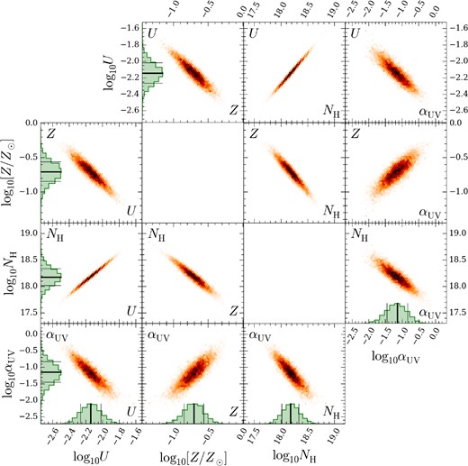
Posterior distributions for component 1. The distribution of MCMC samples is shown as a function of αUV, NH, U (inversely proportional to nH) and Z. Histograms show the marginalized sample distributions for each parameter, and the thin horizontal and vertical lines show the smallest interval containing 68 per cent of these samples. Note that the top-right panels are mirror images of the bottom-left panels.
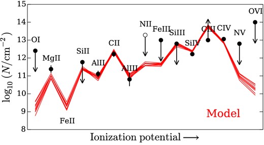
The observed column densities for component 1 and the predicted cloudy column densities for 10 MCMC samples selected at random. Transitions are in order of increasing ionization potential, from left to right. Error bars show the 1σ uncertainties on the measured column densities. The open circles show observed ones that were not used in the parameter estimation.

Parameters in Table 2 plotted as a function of component velocity. The top panel shows the metallicity in comparison to the measurement of the outflowing ISM metallicity in the lensed LBG CB58 (Pettini et al. 2002b) and the metallicity of the background IGM at z = 2.5 (Schaye et al. 2003; Simcoe et al. 2004). The lighter, red points in the αUV plot show components where a prior of αUV = −0.25 ± 0.5 has been applied.
Parameters estimated directly by MCMC sampling (Z, nH, αUV and |${\it N}_\mathrm{H\,\small {i}}$|) and other derived parameters for the eight components we model. The metallicity has a flat prior between −3 and 0.5, the number density has a flat prior between −4 and 0, and αUV has a flat prior between −3 and 2. Bold indicates that value has an additional prior applied: for αUV this is a Gaussian distribution centred on αUV = −0.25 with σ = 0.5, and for |${\it N}_\mathrm{H\,\small {i}}$| it is the |${\it N}_\mathrm{H\,\small {i}}$| measurement in that component. The uncertainties are 1σ, marginalized over all other parameters, and so take into account covariances among the parameters. We include an additional 0.3 dex systematic uncertainty in nH due to the unknown normalization of the incident radiation field. This is propagated to all quantities which are derived from nH: D, mass and P/k. For these quantities, the uncertainty without including this nH systematic is shown in parentheses.
| Vel. | |$\log _{10} {\it N}_\mathrm{H\,\small {i}}$| | log10NH | ||||
|---|---|---|---|---|---|---|
| Comp. | (km s− 1) | log10(Z/Z⊙) | αUV | log10U | (cm−2) | (cm−2) |
| 1 | −112 | −0.70 ± 0.14 | −1.14 ± 0.31 | −2.14 ± 0.12 | 14.88 ± 0.01 | 18.18 ± 0.16 |
| 2 | −84 | −0.39 ± 0.12 | −0.15 ± 0.27 | −2.54 ± 0.09 | 15.23 ± 0.01 | 18.02 ± 0.14 |
| 3 | −30 | −0.34 ± 0.37 | |$\boldsymbol {-0.35\pm 0.42}$| | −1.83 ± 0.19 | 14.47 ± 0.26 | 17.96 ± 0.40 |
| 4 | +51 | −0.35 ± 0.11 | 0.30 ± 0.15 | −2.73 ± 0.12 | 16.43 ± 0.09 | 18.97 ± 0.17 |
| 5 | +72 | −0.21 ± 0.11 | 0.37 ± 0.14 | −2.70 ± 0.11 | 16.37 ± 0.09 | 18.90 ± 0.16 |
| 6 | +92 | −0.26 ± 0.11 | 0.20 ± 0.18 | −2.66 ± 0.10 | 16.02 ± 0.10 | 18.62 ± 0.13 |
| 7 | +235 | −0.69 ± 0.23 | |$\boldsymbol {0.01\pm 0.38}$| | −2.43 ± 0.17 | 14.70 ± 0.01 | 17.64 ± 0.25 |
| 8 | +324 | −1.07 ± 0.42 | |$\boldsymbol {-0.24\pm 0.48}$| | −1.63 ± 0.44 | 13.59 ± 0.01 | 17.76 ± 0.57 |
| Vel. | log10T | log10nH | log10(P/k) | log10D | log10M | |
| Comp. | (km s− 1) | (K) | (cm−3) | (cm−3K) | (kpc) | ( M⊙) |
| 1 | −112 | 4.19 ± 0.03 | −2.85 ± 0.33(0.14) | 1.33 ± 0.32(0.12) | −0.46 ± 0.42(0.30) | 3.55 ± 0.96(0.75) |
| 2 | −84 | 4.14 ± 0.02 | −2.37 ± 0.32(0.12) | 1.78 ± 0.32(0.10) | −1.10 ± 0.39(0.25) | 2.07 ± 0.88(0.64) |
| 3 | −30 | 4.24 ± 0.10 | −3.10 ± 0.38(0.23) | 1.06 ± 0.37(0.22) | −0.45 ± 0.65(0.57) | 3.40 ± 1.64(1.53) |
| 4 | +51 | 4.14 ± 0.03 | −2.11 ± 0.33(0.13) | 2.03 ± 0.32(0.12) | −0.40 ± 0.41(0.28) | 4.45 ± 0.94(0.72) |
| 5 | +72 | 4.11 ± 0.03 | −2.15 ± 0.32(0.12) | 1.97 ± 0.32(0.12) | −0.42 ± 0.39(0.26) | 4.34 ± 0.89(0.66) |
| 6 | +92 | 4.12 ± 0.03 | −2.21 ± 0.32(0.11) | 1.91 ± 0.32(0.12) | −0.65 ± 0.36(0.21) | 3.59 ± 0.80(0.53) |
| 7 | +250 | 4.27 ± 0.04 | −2.46 ± 0.37(0.21) | 1.80 ± 0.35(0.17) | −1.38 ± 0.55(0.46) | 1.17 ± 1.31(1.16) |
| 8 | +324 | 4.49 ± 0.12 | −3.34 ± 0.55(0.46) | 1.09 ± 0.45(0.34) | −0.22 ± 1.08(1.04) | 3.60 ± 2.71(2.64) |
We apply a Gaussian prior in log space to |${\it N}_\mathrm{H\,\small {i}}$| corresponding to the measured column density. For components 1, 2, 4, 5 and 6 the metallicity, spectral tilt and volume density can be constrained independently. For the weaker components 3, 7 and 8, fewer metal lines are detected and these three parameters cannot be independently constrained. Therefore we impose a prior distribution on αUV of a Gaussian centred at −0.25 with σ = 0.5. This prior is consistent with the αUV range measured in the other five components.
The models can reproduce column densities of all the species apart from O vi, including the majority of C iv and Si iv. This suggests that all of this absorption is produced by the same phase, and that there is not a large fraction of C iv associated with the gas producing O vi. The largest discrepancy between the models and data is for Mg ii, which is low by 0.2–0.4 dex in the models for components 1, 4, 5 and 6 (see Fig. 7 and B13–B15). We also observed a Mg ii enhancement in Crighton et al. (2013b), hinting that this could be a common feature of the z ∼ 2.5 CGM. This is unlikely to be caused by more complicated variations in the UV background than those captured by αUV, as Si ii, which has a similar ionization potential, is well modelled in components 4, 5 and 6 (see Figs B13–B15). It could be produced by a departure from solar abundance ratios. However, our favoured explanation is that it is caused by a density variation in the cloud (the cloudy models assume a constant density). If there is a denser core near the centre of the cloud, this could result in stronger very low ion absorption relative to higher ions. Such dense cores are known to exist in some high column density absorbers at lower redshift (e.g. Crighton et al. 2013a). We intend to investigate this scenario further in future work.
The gas metallicity ranges from log10(Z/Z⊙) = −1.1 ± 0.4 for component 8 to log10(Z/Z⊙) = −0.2 ± 0.1 for component 5. The log10U values are between −2 and −3, corresponding to densities of 10−3 to 10−2 cm−3 (assuming |$\Gamma _{\rm H\,{\small {i}}}=0.8\times 10^{-12}$| s−1). These densities are similar to the high-metallicity components in the absorber analysed by Crighton et al. (2013b). As we describe in Appendix B1, these densities are lower limits. If there are any local ionizing sources in addition to a Haardt–Madau UV background, these tend to result in higher densities and thus smaller cloud sizes. The component metallicities are comparable to those measured in the outflowing interstellar medium (ISM) of the lensed Lyman-break galaxy (LBG) MS 1512-cb58 (Pettini et al. 2002b), and much larger than the IGM metallicity at this redshift (Schaye et al. 2003; Simcoe, Sargent & Rauch 2004) as shown in Fig. 8.
Interestingly, components 1, 4, 5 and 6 have a αUV different from zero, suggesting deviations from a HM12 background. Components 1 and 4/5/6 also have very different αUV from each other, which may indicate an inhomogeneous ionizing spectrum across the absorber. It is possible that relative abundance variations or non-equilibrium effects could mimic a non-zero αUV. We have tried introducing departures from solar abundance ratios, but find that the non-zero αUV solutions remain. We defer a discussion on the possibility of a variable ionizing radiation field and departures from a HM12 background to a future paper. For this work, we simply treat αUV as a nuisance parameter that is marginalized over to find the metallicity and density.
If we use a fixed value of αUV we underestimate the uncertainty on the metallicity by a factor of 3. This demonstrates the importance of including a variation in the UV slope when estimating the metallicity.
4 PHYSICAL CONDITIONS IN THE GALAXY's CGM
We have shown that the partial LLS at an impact parameter of 50 kpc from the galaxy is metal enriched to a level seen in the ISM of LBGs, far above the IGM metallicity. The galaxy is faint (0.2 L*) and likely has a low halo mass (∼1011.4 M⊙). All other R < 25.5 BX candidates within 15 arcsec have been targeted with spectroscopy and ruled out as being <1000 km s− 1 from the LAE redshift (Cooksey et al., in preparation; Crighton et al., in preparation). Therefore there is no evidence that this is a satellite in a higher mass halo. The QSO point spread function covers a small solid angle, but it is possible it may hide another z = 2.5 galaxy even closer the QSO sightline (<1.5 arcsec, or <10 kpc). Higher resolution imaging would help to identify any closer galaxy candidates to the QSO sightline.
Even though this is a single galaxy–absorber pair, because this is the first LAE studied in absorption and the pair was not absorption selected, the covering fraction of gas around similar galaxies is likely to be significant. The binomial 95 per cent confidence range for one success from a single observation is 0.2–1, suggesting a covering fraction >20 per cent.9 This is consistent with the association on ∼50 kpc scales between Mg ii and low stellar mass galaxies at z ≈ 1–2 in Lundgren et al. (2011). A large covering fraction of strong H i is also seen in higher mass haloes, around QSOs at z ∼ 2 (Prochaska et al. 2013b) and around BX-selected galaxies at z ∼ 2.3 (Steidel et al. 2010; Rudie et al. 2012). We note the rest equivalent width of Mg ii 2796 is 0.37 Å, which lies close to the empirical ρ–Wr relation found by Chen et al. (2010) at z < 0.5. This is consistent with the idea that the circumgalatic medium extent remains roughly constant from z ∼ 2.5 to z < 0.5 (Chen 2012).
At redshifts <1 Lehner et al. (2013) have discovered a metallicity bimodality for systems with a similar |${\it N}_\mathrm{H\,\small {i}}$| (1016–1019 cm−2) to our partial LLS. The existence of a metallicity bimodality at z > 1 has not yet been established, but it is interesting that the partial LLS component metallicities we measure are all consistent with the high-metallicity branch of this bimodality, which Lehner et al. interpret as being produced by outflowing winds, stripped gas or recycled outflows. In the following sections we explore possible physical origins for the partial LLS.
4.1 Can the absorption be caused by IGM gas?
4.2 Pressure confinement
Therefore the gas we observe may be in pressure equilibrium with an ambient hotter gas halo, but it is unlikely to have condensed out of a static hot halo.
4.3 Inflowing or tidally stripped gas model
If the gas has not condensed from a hot halo, how did it find its way into the CGM? Could it have been pre-enriched at a higher redshift or in a galactic fountain, and now be infalling towards the galaxy, causing the velocity spread we see? Or could it be stripped from the ISM of fainter satellite galaxies?
Such a large covering fraction of small clumps is consistent with a population of high velocity cloud (HVC)-like systems, similar to those observed in the Milky Way's halo, some of which are infalling. On the other hand, simulations generally predict that infalling gas is manifest as a small number of narrow streams (e.g. Fumagalli et al. 2011b; Shen et al. 2013), which seems incompatible with a large covering fraction of small clumps.
Based on the high velocity width of the system we conclude that most of the absorbing components are unlikely to be infalling or stripped, but we cannot rule out some components being caused by inflowing gas.
4.4 Outflowing gas model
An alternative explanation is a supernovae-driven wind. The distance travelled by winds through the CGM is poorly constrained, but the dependence of Mg ii absorption with inclination angle around galaxies at lower redshift suggests they could reach as far as ∼50 kpc (Bordoloi et al. 2011; Bouché et al. 2012; Kacprzak, Churchill & Nielsen 2012). In a wind model the gas metallicity is naturally explained by recent supernovae enrichment, and the large velocity width and high covering fraction is due to an outflowing shell morphology.
We can compare the absorber metallicity to that estimated using emission from H ii regions in z ∼ 2.5 galaxies from Erb et al. (2006). These metallicities are subject to greater systematic uncertainties than those measured from absorption, because only a small number of emission lines can be detected and the metallicity indicators are calibrated at low redshift, but they provide the only direct measurements of gas-phase metallicities in high-redshift galaxies. The mass–metallicity relation from Erb et al. (2006) indicates the metallicity for a z ∼ 2, M* = 109.1 M⊙ galaxy is ∼0.3 solar, similar to the absorber metallicities we measure.
We can also compare to metallicities which are directly measured in outflowing winds from two z = 2.7 lensed LBGs. These lensed galaxies are bright enough to be observed at moderate spectral resolution, enabling the H i and metal column densities to be measured in the blueshifted ISM absorption. The first galaxy is cb58 at z = 2.7, which has an outflowing gas metallicity of ∼0.4 solar (Pettini et al. 2002a). The second is the ‘8 o'clock arc’, another z = 2.7 lensed galaxy (Dessauges-Zavadsky et al. 2010) which has an outflowing gas metallicity of 0.4–0.7 solar. These are both similar to the metallicities we measure in the partial LLS. The 8 o'clock arc outflow metallicity may be higher than that of cb58 and of several of the partial LLS components, but the 8 o'clock arc is a highly luminous galaxy with stellar mass ∼4 × 10¹¹ M⊙, much higher than both cb58 (∼2 × 10¹⁰ M⊙) and the galaxy in this work. Therefore we expect its ISM metallicity to be ∼0.2 dex higher based on the mass–metallicity relation. We conclude that the metallicities we find in the partial LLS are consistent with metallicities directly measured in the outflowing winds of these two z = 2.7 LBGs.
Fig. 9 shows a possible outflow geometry where we have intersected an outflowing cone whose density decreases with increasing radial distance from the galaxy. Such a geometry is observed in lower redshift outflows (e.g. M82; Walter, Weiss & Scoville 2002). Here a large component of the wind velocity is perpendicular to the sightline. The strong central components occur closest to the galaxy in a higher density region of the outflowing shell, and the outer components are produced in lower density regions more distant from the galaxy.
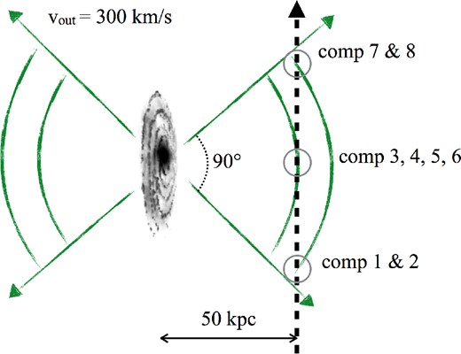
A toy model of an outflow that is consistent with the absorption we observe. The dashed line is the sightline to the background QSO, which passes through a shell of gas outflowing from the nearby galaxy with velocity 300 km s− 1. The density of the gas decreases with radius, meaning the strongest components are produced at the smallest radii from the galaxy. Here we assume an outflow opening angle of 90°, but larger angles are also possible.
4.4.1 Mass outflow rate
Is the SFR of the galaxy consistent with driving such a wind? The galaxy is unresolved in the r′ imaging with 0.6 arcsec seeing, implying it must have a size less than ∼5 kpc. Using the measured SFR of ∼1 M⊙ yr−1 and a half-light radius of 2.5 kpc (typical of z ∼ 2.5 star-forming galaxies; e.g. Law et al. 2012) gives ΣSFR = 0.05 M⊙ yr−1 kpc−2, comparable to the theoretical value required to drive a superwind ∼0.05 M⊙ yr−1 kpc−2 (Murray, Ménard & Thompson 2011). Lower redshift galaxies with similar star formation surface densities have also been observed to drive winds (e.g. Rubin et al. 2013). The formalism presented by Murray, Quataert & Thompson (2005) predicts the momentum deposition (|$\mathrm{\dot{M}} v$|) for a radiatively driven wind from a starburst. This formalism relates the SFR to the momentum deposition by |$\mathrm{\dot{M}} v = 2\times 10^{33}\ \mathrm{SFR}/(\,{\rm M}_{{\odot }}\,{\rm yr}^{-1})\,$|g cm s−2. Using our measured mass outflow rate, the SFR required is ∼5 M⊙ yr−1, five times larger than the observed SFR. However, the observed SFR may not have been the SFR in the galaxy at the time the wind was launched. Starbursts have time-scales of 0.1–1 Gyr (e.g. Thornley et al. 2000; McQuinn et al. 2010). The time for a wind travelling at 300 km s− 1 to reach 50 kpc is 0.2 Gyr, assuming the wind has not deccelerated. Therefore it is possible that a previous starburst event could have launched the wind, then subsequently died away leaving the SFR that we measure. This scenario could be tested by taking a rest-frame optical spectrum of the galaxy, which would show strong post-starburst features, similar to a lower redshift galaxy that shows a large-scale wind in absorption in a nearby QSO sightline (Tripp et al. 2011). Due to the faintness of the galaxy this is challenging with current facilities, but will become straightforward once the James Webb Space Telescope or 30m-class ground-based telescopes become available.
This outflow rate is much smaller than the rate reported by Steidel et al. (2010) at z ∼ 2.3 around BX-selected galaxies (∼230 M⊙ yr−1) and is bracketed by the different estimates from Martin et al. (2012) (∼23 M⊙ yr−1) and Rubin et al. (2013) (∼1 M⊙ yr−1) for a z ∼ 0.7 galaxies with a similar SFR to the galaxy in this work. We caution that in those studies gas absorption features are both saturated and unresolved, |${\it N}_\mathrm{H\,\small {i}}$| cannot be measured and the outflow geometry is not well constrained. This means the gas metallicity, dust depletion, ionization corrections, and thus these outflow rates are uncertain by an order of magnitude or more. The high S/N and resolution of our QSO spectrum allows precise derivations of the |${\it N}_\mathrm{H\,\small {i}}$|, metallicity, dust depletion and ionization corrections, so in the context of an outflow model the largest uncertainties in the outflow rate are due to the wind geometry. However, our analysis uses a single galaxy–absorber pair and substantial uncertainties in the geometry remain.
A larger sample of systems is necessary to confirm the outflow rate we infer here is typical of z ∼ 2.5 galaxies.
4.4.2 Escape velocity
The outflow velocity required by our toy model to reproduce the kinematics of the absorption is 300 km s− 1 at 50 kpc. If the galaxy halo mass is large, ∼1012 M⊙, this is below the halo escape velocity |$\sqrt{2GM_\mathrm{halo}/R} = 410\,\rm km\,s^{-1}$|. However, if the halo mass is 1011.4 M⊙, as suggested by the faint continuum and high Lyα equivalent width, the escape velocity is only 210 km s− 1. In this case the gas we see will escape the potential well of the galaxy to enrich the IGM.
Several lines of evidence point towards low halo mass galaxies being responsible for IGM enrichment (e.g. Madau, Ferrara & Rees 2001; Booth et al. 2012). These imply that galaxies in very low mass haloes, Mhalo ≪ 1011 M⊙, must eject metals to enrich the IGM at high redshift to the level that is observed at z ∼ 3. The galaxy in this work may be the first indication of a low-mass galaxy at z ∼ 2.5 driving metal-enriched gas into the IGM. Near-infrared observations of the galaxy are thus highly desirable to determine whether it has a low stellar mass, as expected from its faint UV magnitude.
4.5 The origin of the O vi absorption
The O vi absorption is shown in the bottom-right panels of Fig. 4, and its parameters are listed in Table 3. While the O vi velocity components are not always precisely aligned with the low ions, they do roughly follow the low-ion components, suggesting a physical connection. Therefore the gas producing O vi is either created by the cool clumps interacting with their environment – for example, by warm gas ablated from the cool clumps as they move through a hot halo, which one possible origin for O vi absorption seen around HVCs near the Milky Way (e.g. Richter 2006) – or else produced by the same starburst event that generated the clumps. This also suggests the O vi gas must have a similar size scale (∼kpc) and metallicity (0.1–0.6 solar) to the lower ionization gas.
The velocity relative to the galaxy redshift, the component redshift, b parameter, column density and their 1σ uncertainties for the O vi components shown in Fig. 4. The uncertainties are taken directly from VPFIT, and do not include errors in the continuum placement.
| Vel. (km s− 1) | z | b(km s− 1) | log 10N(cm− 2) |
|---|---|---|---|
| −109 | 2.462 072(05) | 20.8 ± 0.8 | 13.96 ± 0.01 |
| −42 | 2.462 848(09) | 30.8 ± 1.1 | 14.24 ± 0.02 |
| +13 | 2.463 479(80) | 30a | 13.67 ± 0.04 |
| +35 | 2.463 734(27) | 13.0 ± 2.7 | 13.5 ± 0.2 |
| +58 | 2.464 001(11) | 14.4 ± 1.7 | 13.94 ± 0.07 |
| +90 | 2.464 377(13) | 21.1 ± 1.7 | 13.99 ± 0.04 |
| +240 | 2.466 107(07) | 30a | 13.93 ± 0.01 |
Note:ab value fixed.
The O vi absorption is broader than expected from the low-ion absorption and |$N_{\rm O\,{\small {vi}}}$| is not reproduced by our photoionization models. Therefore it must be in a different phase, distinct from the one we model. This phase could be photoionized, in which case it must have a lower density than the cool clumps to avoid producing large amounts of low-ion absorption. However, Lehner et al. (2014) analyse a sample of 15 Lyman-limit absorbers with associated O vi similar to this system (but without information about the presence of a nearby galaxy), and report a correlation between |$b_{\rm O\,{\small {vi}}}$| and |$N_{\rm O\,{\small {vi}}}$|. That is, they do not find many high NO VI, narrow lines, instead high NO VI systems tend to have large line widths. They argue this is caused by O vi being produced by gas cooling radiatively from a hot (T ∼ 105−6 K) temperature, rather than in photoionization equilibrium, as suggested by Heckman et al. (2002). Several of the O vi components in our system have |$b_{\rm O\,{\small {vi}}}=20{\rm -}30$| km s− 1, corresponding to Tmax = (4–9) × 105 K assuming purely thermal broadening, which is consistent with this scenario.
Simcoe et al. (2006) consider two models to explain the broad O vi in another, similar absorber at impact parameter of 115 kpc from a z = 2.3 galaxy. The first is an outflowing shock front driven by a supernovae wind, and the second is infalling, pre-enriched gas that is shock heated during infall on to the halo. The infall scenario is unlikely for our absorber, because of the large velocity extent of the O vi (360 km s− 1), and because of the close velocity association between it and the low ions.
We conclude that the O vi is likely caused by a warm, ∼105 K gas envelope around the cool photoionized clumps. This may be a component of the outflowing gas, or the result of an interaction of the outflowing gas with a hotter halo that could pressure-confine the clumps. It may be radiatively cooling, and collisionally ionized rather than photoionized.
4.6 Mass in the CGM
The O vi is produced by a separate gas phase, and so contributes an additional mass. The NH associated with this phase can be estimated |${\it N}_\mathrm{H}= {\it N}_\mathrm{O\,VI}/ f_{\rm O\,{\small {vi}}} \times (\mathrm{Z}_{{\odot }}/Z)$|, where |$f_{\rm O\,{\small {vi}}}$| is the fraction of oxygen in O5+ and Z is the gas metallicity. Lehner et al. (2014) use the models of Oppenheimer & Schaye 2013 (see also Gnat & Sternberg 2007; Vasiliev 2011) to show that the maximum |$f_{\rm O\,{\small {vi}}}$| is 0.2 for gas at temperatures >104.5 K. Taking the metallicity to be close to that of the photoionized clumps, 0.5 Z⊙, this implies |${\it N}_\mathrm{H}=10^{19}\,\rm cm^{-2}$| for the O vi phase, similar to the low-ion gas. This echoes results at lower redshift. Fox et al. (2013) found the mass contribution for the O vi phase in a sample of LLSs at z < 1 is also comparable to the mass contribution from low ions.
Therefore the combination of cool photoionized gas and gas associated with O vi contains a baryonic mass of ≳0.8 × 10⁹ M⊙. Using our fiducial stellar mass for the galaxy of 1.4 × 10⁹ M⊙, this represents ∼60 per cent of the mass in stars. The amount of mass in the CGM could be larger if it extends beyond 50 kpc, or if either |$f_{\rm O\,{\small {vi}}}$| or the O vi gas metallicity is lower than we have assumed.
4.7 Implications for the origin of Lyman-limit systems
This absorber falls just below the commonly used criterion for LLSs (|${\it N}_\mathrm{H\,\small {i}}>17.2$|), but is likely to share physical characteristics with them. The covering fraction of z ∼ 2.5 LLS around QSOs has been shown to be high (Hennawi et al. 2006; Prochaska, Hennawi & Simcoe 2013a), and they strongly cluster around the QSOs (Hennawi & Prochaska 2007; Prochaska et al. 2013b). Prochaska et al. (2013b) show that these results suggest that the majority of all LLSs could originate within 1 Mpc of the high-mass haloes (≳ 1012 M⊙) QSOs are believed to populate. Steidel et al. (2010) argue that the extended CGM of Lyman-break selected galaxies may also contribute a dominant fraction of LLSs, based on low-ionization metal absorption extending to an impact parameter of 100 kpc. Rauch et al. (2008) argue that faint LAEs, with line fluxes of a few 1018 erg s−1 cm−2, may be responsible for much of the LLS population. There will be some overlap between these samples (some LAEs may also be LBGs, and may be found close to QSOs, for example). Is there also room for a population of LLSs associated with ∼1011.4 halo mass galaxies?
Fumagalli et al. (2013) consider two simple models that reproduce the LLS incidence to z = 3. In the first, LLSs inhabit the CGM of all galaxies within a halo above a minimum halo mass corresponding to a circular velocity of 200 km s− 1 (below which the CGM gas can easily escape), with the CGM halo extent fixed to the virial radius at z = 2.5. The second uses a lower minimum mass cutoff, motivated by most LLS being caused by accreting gas. Due to its faint rest-frame UV magnitudes, the galaxy in this work is likely in a 1011.4 M⊙ halo, which implies the gaseous CGM of more numerous, fainter galaxies also contribute to the LLS population. This is qualitatively in agreement with recent cosmological numerical simulations (Erkal 2014; Rahmati & Schaye 2014) which predict that most LLSs inhabit haloes with Mhalo <1011 M⊙. The LLS absorption cross-section suggested by Fig. 9 is larger than in these cosmological simulations. The suite of single-galaxy simulations by Fumagalli et al. (2014) also predicts a lower covering fraction fc ∼ 0.15 than we have assumed (fc = 0.5). Some of this difference could be due to this system being a partial LLS: weaker LLSs likely have larger CGM covering fractions (e.g. Rahmati & Schaye 2014). However, perhaps more importantly these simulations cannot yet resolve the hydrodynamics relevant for the movement of these clouds through the CGM, as we discuss in Section 5.3.
5 IMPLICATIONS OF SUBKILOPARSEC SCALE CLOUDS
The characteristic sizes we derive for these clouds (Table 2) are very small: 100–500 pc. These sizes are robust to modelling uncertainties, and include uncertainties in the ionizing field normalization. Such small sizes have important implications for the propagation of these clouds through the CGM, and for numerical simulations of the CGM.
5.1 Cloud disruption by hydrodynamic instabilities
First, there may not be any existing hot gas halo. If this is a low-mass galaxy (Mhalo < 1011 M⊙), then a shock may not yet have formed and halo gas may not be at the virial temperature (Birnboim & Dekel 2003). However, it seems unlikely that the halo is completely free of any gas, and the zoomed simulations of Fumagalli et al. (2014) suggest that some hot CGM gas is in place by z ∼ 2, even in Mhalo ∼ 1011.2 M⊙ haloes. The O vi gas we see also suggests a hot halo is present. Therefore this explanation seems unlikely.
A second possibility is that the cool gas does not actually traverse the distance from the galaxy to its current location in the CGM. Instead it condenses just behind a shock front driven by hot gas in the outflow once the temperature of the front drops enough for radiative cooling to become efficient, as outlined by Simcoe et al. (2006, their section 5.2). This scenario can also explain the O vi absorption as cooling gas found behind the shock front.
Finally, there may be a mechanism that makes the clumps resistant to hydrodynamic instabilities. Such mechanisms have been explored to explain the apparent longevity of HVCs in the Milky Way halo, which share many characteristics with the absorbers we analyse: they are small, cool clouds moving through a hotter halo. Confinement by magnetic fields is one possibility with some observational support (e.g. McClure-Griffiths et al. 2010). The effect of magnetic fields on clouds remains unclear, however, and some simulations suggest they may even hasten cloud disruption (Stone & Gardiner 2007), or strongly suppress the relative velocity between the cloud and surrounding ambient medium (Kwak, Shelton & Raley 2009). The mechanism favoured by Putman, Peek & Joung (2012) for extending the lifetimes of HVCs is the presence of a warm envelope around the cool clouds (observed as O vi absorption around the HVCs) that significantly extends its lifetime. It does this by minimizing both the temperature and velocity gradients between the cloud and the halo, making it resistant to instabilities. We also see O vi in this absorber that is likely caused by a warm gas envelope around the clumps, so this is a plausible explanation.
To our knowledge, numerical simulations have not yet been performed to test whether such a warm envelope can indeed extend the cloud lifetime by the necessary amount.
5.2 Small gas clump sizes are a generic feature of the CGM
The absorbing clumps’ small size makes them challenging to resolve in simulations of the CGM. First, we emphasize that there is a large body of evidence indicating that low-ion metal absorbers and partial LLSs have sizes much smaller than a kiloparsec. Using lensed QSO sightlines separated by 10 s of parsecs, Rauch, Sargent & Barlow (1999) showed that a z ∼ 2, |${\it N}_\mathrm{H\,\small {i}}=10^{16}\,\rm cm^{-2}$| system with low-ion metal absorption must have a size <50 pc. Petitjean et al. (2000) found Mg ii systems at z = 1–2 must have sizes <1 kpc due to partial covering of lensed images of a background QSO. Simcoe et al. (2006) found sizes 10–100 pc for components in a partial LLS at an impact parameter of 115 kpc from another z ∼ 2.3 galaxy using photoionization modelling. By inferring the gas density from C ii* absorption, Prochaska & Hennawi (2009) found similar sizes for gas clumps in a LLS in the CGM of a z ∼ 2.5 QSO. Schaye et al. (2007) find small sizes for z ∼ 2.5 metal-rich absorbers selected by their strong C iv and weak H i, again using photoionization modelling. Such small sizes are also found at low redshift: HVCs, with similar |${\it N}_\mathrm{H\,\small {i}}$| to LLS, have sizes <100 pc (Ben Bekhti et al. 2009) inferred from H i 21cm images, and photoionization modelling of gas around z ∼ 0.1 galaxies (Stocke et al. 2013; Werk et al. 2014), of z < 1 LLSs (Lehner et al. 2013) and of weak Mg ii systems (Rigby, Charlton & Churchill 2002) also yields small sizes. Therefore these small clump sizes are a generic feature of both the high- and low-redshift CGM.
Moreover, for the partial LLS in this work it is not only the metals, but also the majority of the H i gas that is confined within a small cloud. Schaye et al. (2007) posit a scenario where tiny, very metal rich clumps populate H i clouds in the IGM. In this scenario, these small metal clumps are responsible for the metals seen in high |${\it N}_\mathrm{H\,\small {i}}$| absorbers, which can have much larger sizes than the clumps. However, there is no evidence that this is the case for the absorbers we see: the H i component velocities are extremely well aligned with the low ions (see Fig. 4), and the photoionization models effectively reproduce the observed column densities of both metals and H i.
5.3 Requirements for numerical simulations of the CGM to resolve these clouds
What are the requirements to resolve the hydrodynamic instabilities affecting these clouds? The situation is comparable to the ‘blob test’ performed by Agertz et al. (2007), where a test case of a dense spherical clump of gas travelling through a diffuse medium is considered using both adaptive mesh refinement (AMR) and smoothed particle hydrodynamics (SPH) simulations. Agertz et al. find that seven adaptive mesh resolution elements per cloud radius are needed to begin resolving the hydrodynamic instabilities which destroy the clump. We adopt an optimistic minimum requirement of three resolution elements per clump radius. Assuming a radius of 400 proper pc – at the upper end of our measured sizes – this implies a minimum cell size of 140 pc. Therefore AMR simulations must refine to this scale in the CGM at densities of 10−3–10−2 cm−3. In existing AMR simulations such small refinement scales can be reached, but only for the highest density regions with ∼1 cm−3.
We conclude that to date, no single galaxy or cosmological simulation has been performed at a sufficient resolution to predict the properties of low-ion gas in the CGM. The best approach for future simulations may be to abandon the attempt to resolve these gas clumps altogether. Instead a subgrid model for their behaviour could be introduced, in the same way that subgrid models are used to treat star formation and galactic-scale outflows in these simulations.
6 SUMMARY
We have serendipitously discovered a faint, 0.2 L*, galaxy at z = 2.466 that is at a small impact parameter (50 kpc) from a background QSO. Based on similarities to galaxies selected as Lyα emitters, it likely has a halo mass ∼1011.4 M⊙ and stellar mass <1010 M⊙.
A very high quality UVES spectrum of the QSO reveals a partial LLS at the galaxy redshift. The absorber shows low- and high-ionization potential transitions in several components spanning a velocity width of 436 km s− 1. As this galaxy–absorber pair was not selected based on the absorber properties, it is likely that the covering fraction of such absorbers around similar z = 2.5 galaxies is significant. Our results can be summarized as follows.
Using a new method to marginalize over uncertainties in the shape of the incident UV field, we measure the density and metallicity of each absorbing component. A single photoionized gas phase can explain all of the low-ionization absorption we see. The gas has a metallicity, Z = 0.1–0.6 Z⊙, similar to the ISM of z ∼ 2.5 galaxies. The gas temperature is cool (104 K) with densities 10−3 to 10−2 cm−3.
Infalling or tidally stripped gas is unlikely to explain all of the absorption, due to the large velocity width and large covering fraction of the gas. Our favoured model is an outflowing shell of gas. If most of the gas we see is in an outflow, the mass outflow rate implied is ∼5 M⊙ yr−1 with a factor of ∼4 uncertainty due to an unknown outflow geometry. This is similar to outflow rates measured around galaxies with halo mass 1011–1012 M⊙ at redshifts z ∼ 0.7 using ‘down-the-barrel’ Mg ii absorption against background galaxies.
O vi gas is present with a broader line width than expected from the low ions, and a higher NOVI than predicted by our photoionization models. It must be produced by a different gas phase that is physically associated with the photoionized gas. This phase may be explained by a warmer, possibly radiatively cooling, envelope around the cooler, photoionized gas.
The total gas mass in the 104 K, photoionized phase and the different phase traced by O vi is comparable. Together they imply a baryonic mass >0.8 × 10⁹ M⊙ in the galaxy's CGM. The mass could be much higher if the halo extends further than 50 kpc, the covering fraction of gas is larger than 50 per cent, or if we use less conservative assumptions about the O vi fraction and metallicity.
The photoionized clumps have sizes ranging from 100–500 pc. The uncertainties in these size estimates take into account uncertainties in the shape and normalization of the UV background radiation. Kelvin–Helmholtz instabilities imply that the lifetime of clumps this size moving through a more diffuse halo are very short. Therefore, we suggest that there must be a mechanism present to make the clumps resistant to these instabilities, such as a warm gas envelope surrounding them. The O vi absorption may be produced by such an envelope.
The small clump size makes them very difficult to resolve in numerical simulations. No single-galaxy or cosmological simulation performed to date has the resolution necessary to correctly treat the movement of the clumps through the CGM. We suggest that a CGM subgrid model capturing the relevant physics may be necessary for future simulations.
In our outflow model, the wind velocities required to explain the kinematics exceed the escape velocity of a 1011 M⊙ halo. In this case the metal-enriched gas will escape into the IGM.
This final result hinges on the galaxy having a halo mass lower than is typically measured for brighter z ∼ 2.5 galaxies. We argue this is likely to be the case based on the large Lyα equivalent width and faint rest-frame UV continuum. However, deep IR imaging would allow more robust SED modelling of the galaxy to give a more precise measurement of the stellar and halo masses.
Finally, the new integral field unit now available on the ESO VLT, Multi Unit Spectroscopic Explorer (MUSE), has the capability to find similar weak emission line galaxies around QSO sightlines at higher redshifts. We expect MUSE will be able to efficiently assemble a large number of similar systems over the redshift range 3–5.
We thank the referee for their helpful comments which improved the paper. Yujin Yang provided helpful correspondence, and Elisabeta Da Cuhna generously provided electronic versions of the tables in her paper. We also thank Richard Bielby, Charles Finn, Simon L. Morris and Kate Rubin for their comments on an earlier draft. This work was based on observations carried out at the European Southern Observatory (ESO), under programmes 166.A-0106, 185.A-0745 and 091.A-0698. We particularly thank the Paranal Observatory support staff for their help with the visitor-mode observations taken for programme 091.A-0698. Our analysis made use of astropy (Astropy Collaboration 2013),12xidl,13DS914 and the NASA/IPAC Extragalactic Database (NED).15 Plots were made with matplotlib (Hunter 2007)16 and aplpy.17 NC and MM thank the Australian Research Council for Discovery Project grant DP130100568 which supported this work. MF acknowledges support by the Science and Technology Facilities Council [grant number ST/L00075X/1].
Data and code used for this paper are available at https://github.com/nhmc/LAE; doi:10.5281/zenodo.12321
We define a partial LLS as having an optical depth <1 at the Lyman limit.
Available for download from http://code.google.com/p/igmtransmission
These programmes observed this QSO due to its extreme luminosity and the presence of strong metal line systems at redshifts unrelated to the galaxy we study in this work.
Written and maintained by MTM at http://astronomy.swin.edu.au/mmurphy/UVES_popler.
The ionization potential is the energy required to remove the outer electron of a species.
There could be a publication bias here: other groups may have discovered a similar galaxy close to a QSO sightline without an absorber and declined to publish the result. We are not aware of any unpublished systems, but this effect is difficult to quantify.
For a clumpy outflow, NH in equation (5) is the mean NH over the shell area, averaging over clumps.
Using the number density for Lyα emitters (Hayes et al. 2010) with a similar Lyα luminosity to our galaxy does not change our conclusions.
REFERENCES
APPENDIX A: VIRIAL RADIUS, TEMPERATURE, AND VELOCITY
APPENDIX B: ESTIMATING PHYSICAL PARAMETERS FROM CLOUDY MODELLING INCLUDING AN UNCERTAINTY IN THE SHAPE OF THE IONIZING RADIATION
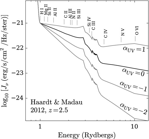
The effect of different αUV on the shape of the integrated QSO and galaxy background radiation. αUV = 0 gives the fiducial HM12 background spectrum at the redshift of the absorber. αUV > 0 makes the slope more shallow (giving a harder spectrum) while αUV < 0 makes it steeper (softer). The ionization potential of the observed transitions is also shown.
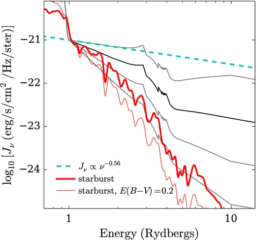
Comparison between QSO-dominated and galaxy-dominated radiation fields, and our parametrization. The dashed line shows a hard QSO spectrum with spectral index −1.5. The thick red line shows a smoothed spectrum of starburst galaxy generated using Starburst99. Then thinner red line below shows the same spectrum with the extinction from Calzetti et al. (2000) applied, assuming E(B − V) = 0.2, typical of z = 2.5 LBGs (Reddy et al. 2008). The range of αUV we consider covers both these extreme cases. The black and grey lines are the same as those shown in Fig. B1.
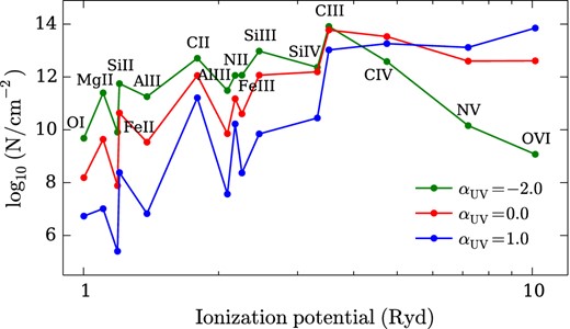
The effect of different αUV on predicted column densities. The predicted column densities are plotted as a function of the species ionization potential for a fixed metallicity, nH and |${\it N}_\mathrm{H\,\small {i}}$|, only varying αUV. As αUV becomes more negative (giving a softer ionizing spectrum), the column density of low ionization potential species (left) increases with respect to higher ionization potential species (right).
This is a simple parametrization of the spectral shape. A model for the UV background with three or more free parameters has also been proposed by Fechner (2011) and Agafonova et al. (2007). However, we prefer a one-parameter model for two reasons: first, the absorbers we model do not show enough metal transitions to effectively constrain more than one parameter and secondly, it is computationally simpler to evaluate. Fig. B2 shows how this parametrization compares to the largest and smallest slopes expected for the ionizing spectrum: αUV = −2 gives a spectral shape close to that expected for a starburst galaxy with dust extinction, whereas αUV = 1 corresponds to the largest power-law slope observed in spectra of QSOs in the 1 to 4 Ryd range (Scott et al. 2004; Shull, Stevans & Danforth 2012). Therefore our one-parameter model captures the range of uncertainty in the shape of the ionizing spectrum relevant to the 1–10 Ryd region.
For observed column density measurements, we assume the likelihood is a Gaussian with two discrete σ width parameters, one each for the upper and lower uncertainties. For upper limits we assume a step-like function with a one-sided Gaussian of fixed σ = 0.05 dex describing the likelihood above the upper limit. We use an analogous function for lower limits. When calculating the likelihood of a set of model parameters we apply a minimum uncertainty in log10 of the observed column densities of 0.1 dex. This allows for the fact that there could be (a) more complicated shapes for the UV background than our single-parameter model can capture, (b) minor abundance variations, (c) non-equilibrium effects, (d) geometric effects or (e) density variations across the cloud, which would all perturb the column densities from the equilibrium, constant density, solar abundance models that cloudy calculates. It also prevents one or two observed values with very small uncertainties from dominating the final solution. Applying a minimum uncertainty of 0.15 or 0.05 does not significantly change our results.
For all the components we analyse here, |${\it N}_\mathrm{H\,\small {i}}$| can be precisely measured. Therefore we apply a Gaussian prior to |${\it N}_\mathrm{H\,\small {i}}$| given by the measurement and uncertainty on |${\it N}_\mathrm{H\,\small {i}}$|. For components 2, 7 and 8, where αUV is poorly constrained, we also apply a Gaussian prior to αUV. Limited ranges in log10(Z/Z⊙) (−3 to 0.5), log10nH (−4.5 to −1), |$\log _{10}{\it N}_\mathrm{H\,\small {i}}$| (13 to 17.5), and αUV (−2.5 to 1) are also imposed, which act as another effective prior.
As a test that our method can reproduce the results of previous cloudy analyses, we applied it to components in Crighton et al. (2013b) and Simcoe et al. (2006), applying a strong prior on αUV equivalent to fixing the incident radiation field shape. We verified that the densities and metallicities we infer are consistent with the values found by those analyses, given the ionizing spectral shapes they assumed (HM12 or starburst-dominated for Crighton et al., and a Haardt–Madau background combined with starburst spectrum for Simcoe et al.).
B1 Normalization of the incident radiation field and He ii constraints
The comparison between observed column densities and cloudy models usually gives tight constraints on the ionization parameter, U. These can be related to the density nH using equation (B2). However, a higher nH value can always be compensated by a higher normalization for the incident radiation field, leaving U unchanged. Therefore there is an additional uncertainty in nH due to the uncertainty in the normalization of the incident radiation field.
For a given value of αUV we normalize the ionizing spectrum such that the photoionization rate, |$\Gamma _{\rm H\,{\small {i}}}$|, matches the value measured by Faucher-Giguère et al. (2008) for the integrated UV background from QSOs and galaxies at z = 2.5. The uncertainty in this depends not only on measurement errors, but also on assumptions about the thermal history of the IGM. For example, Becker & Bolton (2013) find a |$\Gamma _{\rm H\,{\small {i}}}$| ∼0.3 dex higher than Faucher-Giguere et al. by assuming a different thermal history. To take into account this uncertainty, we adopt an additional uncertainty of 0.3 dex for our nH estimates, which we add in quadrature to the uncertainties estimated from our MCMC procedure. It is also possible that the true radiation field could be much stronger than this if there are local ionizing sources from an AGN or starburst. This is unlikely for the absorber in this work, because the nearby galaxy has a modest SFR and shows no evidence for an AGN, but it remains a possibility. It implies that the normalization we assume for the radiation field is a lower limit, as local sources can only add to the background radiation field. Therefore our nH measurements are lower limits, and our inferred cloud sizes and masses are upper limits. Local sources can also change the shape of the ionizing spectrum, as shown in Fig. B2. However, the range of αUV we marginalize over covers the expected slopes from dusty starburst-dominated to QSO-dominated shapes over the 1–10 Ryd range, so while there could be small-scale variations in the shape of the radiation field due to local sources which our slope parametrization does not capture, we do not expect this to strongly bias the derived nH.
Since we normalize the incident radiation for each value of αUV independently, the conversion multiplier between nH and U is not the same for different ionizing spectrum shapes. We use spline interpolation to find the nH to U conversion factors when calculating U from our nH parameter samples.
SUPPORTING INFORMATION
Additional Supporting Information may be found in the online version of this article:
Figure B4. Posterior distributions for component 2.
Figure B5. Posterior distributions for component 3.
Figure B6. Posterior distributions for component 4.
Figure B7. Posterior distributions for component 5.
Figure B8. Posterior distributions for component 6.
Figure B9. Posterior distributions for component 7.
Figure B10. Posterior distributions for component 8.
Figure B11. 10 MCMC samples for component 2.
Figure B12. 10 MCMC samples for component 3.
Figure B13. 10 MCMC samples for component 4.
Figure B14. 10 MCMC samples for component 5.
Figure B15.10 MCMC samples for component 6.
Figure B16.10 MCMC samples for component 7.
Figure B17.10 MCMC samples for component 8 (Supplementary Data).
Please note: Oxford University Press are not responsible for the content or functionality of any supporting materials supplied by the authors. Any queries (other than missing material) should be directed to the corresponding author for the paper.
