


Abstract
We report on a pilot study of a novel observing technique, defocused transmission spectroscopy, and its application to the study of exoplanet atmospheres using ground-based platforms. Similar to defocused photometry, defocused transmission spectroscopy has an added advantage over normal spectroscopy in that it reduces systematic errors due to flat-fielding, point spread function variations, slit-jaw imperfections and other effects associated with ground-based observations. For one of the planetary systems studied, WASP-12b, we report a tentative detection of additional Na absorption of 0.12 ± 0.03[+0.03] per cent during transit using a 2 Å wavelength mask. After consideration of a systematic that occurs mid-transit, it is likely that the true depth is actually closer to 0.15 per cent. This is a similar level of absorption reported in the atmosphere of HD 209458b (0.135 ± 0.017 per cent; Snellen et al. 2008). Finally, we outline methods that will improve the technique during future observations, based on our findings from this pilot study.
1 INTRODUCTION
The study of exoplanetary atmospheres has become one of the fastest developing fields of astronomy in the last 10 years. Planetary atmosphere detection and characterization have been achieved primarily using three methods – multi-waveband transit photometry, secondary eclipse photometry, and transmission spectroscopy. Multi-waveband transit photometry involves primary transit observations in several wavelengths simultaneously. This probes to various depths in the exoplanet atmosphere, meaning the transit light curve in each band can be fit in order to detect the difference in planetary radius due to the transmission signal in the atmosphere (e.g. Haswell et al. 2012; Southworth et al. 2012; Copperwheat et al. 2013). Secondary eclipse photometry provides information on the thermal emission from the surface of the planet itself. Observations of the secondary eclipse of hot-Jupiters in the visible and NIR (e.g. Anderson et al. 2010; Gibson et al. 2010; Burton et al. 2012) allow for the brightness temperature to be calculated, an essential parameter for models of atmospheric simulations and dynamics. Transmission spectroscopy enabled the first detection of a hot-Jupiter exoplanet atmosphere (Charbonneau et al. 2001) where sodium was detected in the atmosphere of the transiting planet HD 209458b. This is a technique where the in- and out-of-transit spectra are compared and, depending on which absorbing species are present in the planetary atmosphere, their presence can be determined by a deepening of the absorption features in the spectrum. Sodium is often studied due to the large relative signal it creates during transit relative to the surrounding continuum. In addition, the Na abundance can be probed to different depths, proving information on the temperature–pressure (TP) profile of the atmosphere (e.g. Vidal-Madjar et al. 2011; Huitson et al. 2012). The technique of transmission spectroscopy has since been carried out on a number of hot-Jupiter exoplanets, both from space-based platforms (Sing et al. 2008; Knutson et al. 2011; Crouzet et al. 2012; Madhusudhan et al. 2014; Nikolov et al. 2014), and from the ground (Snellen et al. 2008; Bean et al. 2011; Crossfield, Barman & Hansen 2011; Mancini et al. 2013; Danielski et al. 2014).
Due to the contested nature of some of the detections of absorption features present in exoplanet atmospheres (Swain, Vasisht & Tinetti 2008 versus Gibson, Pont & Aigrain 2011; Tinetti et al. 2007 versus Ehrenreich et al. 2007), it is imperative that any sources of uncertainty due to systematics are well-understood and characterized. Methods to mitigate such sources of uncertainty will allow for characterization of smaller exoplanets, in addition to planets orbiting fainter host stars. Multiple observations of such systems will allow for any claim of atmospheric detection to be verified by independent studies. The characterization of hot-Jupiters will also allow for any potential classification systems which are based on atmospheric constituents (e.g. pM/pL – Fortney et al. 2008, C/O ratio – Madhusudhan 2012) to be thoroughly tested, and provide much needed observational data points with which to test theories of exoplanet atmospheres (Marley et al. 2013). In regard to this, WASP-12b (Hebb et al. 2009) is an ideal candidate for carrying out such tests. WASP-12b is a 1.4MJ planet orbiting a G0-type star, on an orbital period of 1.09 d. It is one of the hottest known hot-Jupiters, with an equilibrium temperature of ∼2500 K. Previous investigations into WASP-12b have revealed a high C/O ratio (Madhusudhan et al. 2011; Stevenson et al. 2014), in addition to a transmission spectrum lacking in TiO features (Sing et al. 2013). Such results are important aspects in testing classification systems due to the predictions of atmospheric constituents which should be detectable in hot-Jupiter atmospheres. Recently, it has been discovered that WASP-12 is part of a triple system (Crossfield et al. 2012; Bergfors et al. 2013), meaning that analysis must take into consideration blending with the two M-dwarf companions.
We propose a method of spectroscopic observation which aims to furnish the detection of exoplanet atmospheres from ground-based systems, while reducing the impact of systematics and errors arising due to flat-fielding and slit-loss corrections. In this paper, we report a pilot study of a search for additional Na absorption in three exoplanet atmospheres. Section 2 describes the method we adopted for our technique. Section 3 details the observation runs for the pilot study. Section 4 describes the data reduction. Section 5 describes the extensive data analysis we conducted, including our search for systematics and the Na analysis in the atmosphere of WASP-12b. Section 6 discusses the technique in wider context to future work and follow-up studies. Section 7 contains our recommendations for future observations utilizing the technique, and finally, we provide some preliminary conclusions on the results from our pilot study.
2 METHOD
The typical precision required to detect an exoplanet atmosphere is of the order of ∼0.1 per cent. Due to the systematics associated with ground-based observations, the technique of transmission spectroscopy provides a unique challenge. How does one minimize the impact of systematics on observations whilst searching for an extremely small signal? In a technique similar to defocused photometry, we present the technique of ‘defocused transmission spectroscopy’. As with defocused photometry, the aim of defocused spectroscopy is to spread the light over a larger number of pixels on the CCD in order to reduce flat-fielding errors, variations due to seeing, and other systematic sources of noise such as tracking errors. In contrast to high-resolution transmission spectroscopy, this method aims to maximize the signal-to-noise ratio (SNR) achieved from the ground. Since we are attempting to characterize a strong individual spectral line, as opposed to the more subtle individual spectral features, our aim is simply to maximize the SNR whilst using defocusing to minimize systematics. This makes the technique ideal for less-bright targets that high-resolution spectroscopy has been unable to study in the past. In order to detect the hot-Jupiter atmospheric features, particular lines in the spectrum are selected (e.g. Na), which are then compared to the surrounding continuum during transit. Any changes in the line depth due to the atmosphere annulus transiting the host star can then be detected by comparing the in- and out-of-transit line depths directly. This method can be applied to any ground-based set-up for both low- and high-resolution spectroscopy.
2.1 Simulations
In order to investigate the effect of defocusing on systematic errors present in transmission spectroscopy observations, we carried out a simulation. Fig. 1 shows a comparison between two simulated spectra, one with no defocusing and another defocused to 2.48 arcsec with a slit width of 2.48 arcsec, the widest slit possible with an instrument like the Intermediate dispersion Spectrograph and Imaging System (ISIS) on the William Herschel Telescope (WHT), whilst maintaining adequate resolution (as obtained by Charbonneau et al. 2002). We aimed to use the widest slit possible to reduce slit-losses due to differential refraction, as well as reducing the impact of any imperfections of the slit jaws that interfere with the beam.
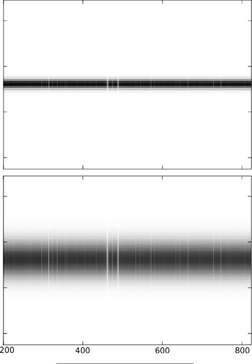
Top: spectra in focus with a slit-width of 2.48 arcsec. Bottom: spectra defocused to 2.48 arcsec. Both simulations include the effects of variable seeing conditions, slit-jaw imperfections, flat-fielding errors and telescope tracking errors. The two bright lines in the centre of each image correspond to the Na doublet. The x-axis displays the pixels on the detector, and we have assumed a dispersion of 0.22 Å per pixel for the simulations.
One major source of systematic noise during observations arises due to the motion of the spectrum over the CCD due to variations in seeing and drifts in position caused by tracking errors and flexure (e.g. due to temperature variations). This not only causes the spectrum to broaden and narrow in the spatial direction over consecutive exposures, but also moves the spectrum over different pixels. This can result in different spectra being incident on completely different pixels over subsequent observations. The aim of defocusing is to keep the bulk of the spectrum on the same pixels over the course of observations, and any motion that would cause the spectra to move on to pixels with different responses will have a much less significant effect. Furthermore, any change in the seeing will result in a smaller change compared to in-focus observations due to the spectrum spreading on to a smaller fraction of adjacent pixels.
The model spectra in Fig. 1 were generated using an observed solar spectrum convolved with a Gaussian in the spatial direction to simulate the effects of seeing and defocusing. The contribution of the broadened spectrum to each pixel in the simulation was then calculated, and then a pixel sensitivity map was used to mimic flat-fielding errors. Slit-jaw imperfections were modelled by simulating the impact of grains of dust up to 0.5 μm, and the fraction of light blocked off at the specific spatial location was multiplied by the intensity at the corresponding spectral position. The λ−1/5 wavelength dependency of the full width at half-maximum (FWHM) of the seeing profile was also taken into account. Tracking errors here used the typical errors found in WHT observations (up to 0.3 pixels), and flat-fielding errors were at the 0.5 per cent level in order to account for additional sources such as scattered light. Finally, seeing variations were modelled as having an FWHM that was randomly varied assuming a Gaussian distribution of 1.3 ± 0.3 arcsec. In comparison to the focused simulations, defocusing reduced the impact of systematic errors by an order of magnitude, well within the precision required for an Na detection in the atmosphere of a hot-Jupiter exoplanet such as WASP-12b.
2.2 Search for Na
As mentioned earlier, Na is particularly targeted for ground-based studies due to its expected strong signal during transit. In addition, Na is a very narrow feature as opposed to the comparatively broad absorption bands of molecules such as CH4, H2O, TiO and VO. These molecular features are much more difficult to detect compared to the sharp Na doublet absorption lines (located at 5890 Å and 5896 Å), even when using space-based instruments such as the HST/STIS. When testing potential classification systems – such as the pM/pL system proposed by Fortney et al. (2008) – Na is an important distinguishing element between the two atmosphere classes. Similar to M and L class stars, pM and pL class planets were proposed based on their atmospheric constituents. pL class planets have a sufficiently low temperature to cause Ti and V to condense out lower down in the atmosphere. pM class planets, however, have a higher temperature, meaning gaseous TiO and VO can exist higher in the atmosphere. As TiO and VO are very efficient absorbers of incident flux, this leads to pM class planets having anomalously bright day sides (due to a temperature inversion in the stratosphere caused by TiO/VO absorption), as well as the Na absorption feature being suppressed. This means for pM class planets, the level of Na absorption should be reduced, and hence should not be detectable in transmission spectroscopy observations. Na also has a history of being detected in hot-Jupiter atmospheres, both from the ground and space (Charbonneau et al. 2002; Snellen et al. 2008; Sing et al. 2008; Redfield et al. 2008; Sing et al. 2012 Nikolov et al. 2014).
3 OBSERVATIONS
Over all observations, we used the ISIS red arm with QuCAM mounted on the WHT with the R1200R grating. When observing in ‘fast’ mode, QuCAM has the ability to employ an electron multiplying CCD (EMCCD) amplifier. The advantage of using an EMCCD is that one can achieve excellent image quality with a short exposure time through the use of the EM gain register. This amplifies the signal in each pixel before reading out the image, and is used in both photometry and spectroscopy for this very reason. The EM-gain also has the advantage of having a very low effective read noise, something which benefits our specific observations since we are spreading the light over a larger number of pixels. Another advantage of using QuCAM is the extremely short read-time, giving negligible dead-time between subsequent exposures. Not only does this increase the efficiency of the observations, effectively boosting the SNR obtained, but also allows shorter exposures to be used with little loss in on-target time. The ability to use shorter exposures is useful for two reasons; first it enables any relatively rapid variability due to systematics to be monitored and, secondly, it minimizes the potential for cosmic ray hits on the regions of interest that would potentially render individual spectra unreliable at the precisions required.
We decided against performing relative spectroscopy by placing another star on the slit as we wished to prevent introducing potential systematics due to differential refraction. Instead, we chose to keep the slit orientated with the parallactic angle and measure the strength of the Na region compared to a relatively featureless region of nearby continuum, as previously implemented by Snellen et al. (2008), for example. We opted to use the relatively featureless continuum region bluewards of Na (from 5680-5885 Å) as our comparison as Sing et al. (2008) found a source of additional absorption in the redwards continuum of HD 209458b that, if present in our targets and used as the comparison region, would effectively reduce the contrast of any additional Na absorption. The observational setup had a total wavelength coverage of 5680–5920 Å, with the Na doublet being positioned near the red-end of the spectral range for the above reason. During these observations, the dichroic was removed in order to reduce systematics due to ghosting, an issue known to occur when using the dichroic in ISIS. We also opted to use the red arm, again to reduce systematics, as this meant that the light path did not have to be split off at an angle – as would have been the case if we were to have used the blue arm. The slit of 2.48 arcsec projects to 8 QuCam pixels, with the R1200R grating (taking anamorphic magnification into account), and assuming a dispersion of 0.22 Å per pixel, this gives 1.76 Å for the 8 pixel projection.
WASP-12 was observed over three nights from 2010 February 2 to 4. Due to the short orbital period of this exoplanet system, primary transits of WASP-12b were visible on all nights. Unfortunately, the first night was lost due to bad weather. The remaining two nights were clear, and transits of WASP-12b were obtained on both nights, along with 1.3 h of out-of-transit data on February 3 and 1.2 h on February 4. On February 4, we ended observations during transit due to the position of the object on the sky. Upon further investigation, it was discovered that the February 4 data were subject to additional instrumental effects due to changing the CCD control head. Due to this, in addition to having to end observations mid-transit, we opt to concentrate solely on the February 3 data in our search for Na absorption. During this night's observations, we were forced to abandon a large series of data during ingress due to an issue with the telescope control system. The ‘fast’ observing mode deletes any data taken during a run which you are forced to abort, a significant factor in our decision to switch to ‘slow’ during the subsequent observations. We note here that every time we moved off target (e.g. to observe a telluric standard) we took an arc exposure. This allows for the wavelength drift over the chip to be tracked throughout the night, and provides a wavelength calibration for all spectra. For these observations, we defocused the spectra to an FWHM of 12 pixels, corresponding to 2.4 arcsec.
HD 189733 and HD 209458 were observed on the nights beginning 2010 September 5 and 6. Here, the observing run was marred by bad weather and variable observing conditions throughout. The most poorly affected time was during the transit of both objects. After looking at the available data, it became clear that the in-transit spectra were too badly affected to get a detection from. Nonetheless, the out-of-transit data were still used in order to test for systematic effects and is presented. Throughout all observations, we aligned the slit with the parallactic angle in order to reduce differential refraction, and, as during the previous observing run, we defocused to an FWHM of 12 pixels at the start of observations. A summary of all observations is provided in Table A1.
4 DATA REDUCTION
The data were reduced using the pamela spectra reduction suite.1 Prior to input into pamela, all science images were de-biased and flat-fielded. Flat-fields for the spectra were created using a tungsten lamp directly in the path of the beam in order to generate the uniform source of light for each frame. A masterflat was created by median-stacking the individual frames and subsequently removing the spectral response of the lamp using a polynomial fit. An optimal extraction was used in order to produce individual sky background fits for each exposure. This recipe was followed for each exposure for every object. We note here that for some HD 209458 observations, a nearby star appears present on the slit. In these cases, the offending object was masked out during reduction. The extracted data were then wavelength calibrated using an interpolation between the two nearest arcs in time surrounding the spectra. Residual wavelength shifts were still visible in the data after applying the arc calibration. In order to correct for this, we cross-correlated the data (using an out-of-transit high SNR spectra as a template), and then removed the residual shifts given by the cross-correlation function. This is important given the method of measuring absorption we have chosen to adopt (see Section 5.2 for details), whereby we define a window around the Na doublet and integrate the flux under the spectrum. If, however, our wavelength calibration is incorrect, there is a potential to shift the Na line out of the window, or shift part of the continuum into the window. This could potentially have the effect of causing the Na depth to vary over subsequent spectra due to this motion.
5 DATA ANALYSIS
The analysis of the spectra of our targets was carried out following the general approach undertaken by other transmission spectroscopy studies (e.g. Sing et al. 2008; Snellen et al. 2008). In these studies, the strength of the absorption was measured relative to a continuum window, and the in- and out-of-transit depths compared. For these purposes we integrated the flux under the spectra, covering pre-defined wavelength windows. Any change in the flux ratio during transit may be indicative of additional Na absorption due to the exoplanet atmosphere. The data were analysed using the molly spectrum analysis software.1
5.1 HD 189733 and HD 209458
As mentioned in Section 3, the in-transit data for HD 189733b and HD 209458b were badly affected by variable cloud cover, poor seeing and adverse weather conditions. Therefore, we opted instead to analyse the systematics associated with our observing technique for the out-of-transit data obtained during these two nights instead.
One of the main issues when carrying out transmission spectroscopy is the linearity of the detector. If the instrumental response causes the deep Na features to appear shallower due to the non-linearity of the detector, an absorption signal can easily be mimicked. Snellen et al. (2008) investigated non-linearity effects for their High Dispersion Spectrograph (HDS) data of HD 209458 by comparing the normalized continuum count level with the measured mean depth of 59 identified absorption lines. This indicates a strong inverse correlation (i.e. for deeper absorption lines, the higher the flux level in the continuum). In order to perform this analysis, a significant number of absorption features are required, something which we are lacking due to the relatively narrow wavelength coverage we have for our observations. An excellent way in which to characterize the linearity is to obtain flat-fields of different exposure lengths. This gives a uniform response to a range of count levels, and can be used to construct a correction factor if needed. Unfortunately, we neglected to obtain flat-fields of varying exposure time for our data. We are able, however, to use the variable count levels obtained during periods of poor weather to mimic this effect. We did this by first grouping spectra into differing flux levels, and performing an analysis for two different continuum windows with wavelength ranges 5720–5790 Å and 5790–5860 Å (hereafter referred to as C1 and C2, respectively). For a completely linear detector, the slope of the continuum should remain constant over all levels of flux. Fig. 2 shows the continuum window C1 against the ratio of C1 to C2. Note that Fig. 2 shows flux values for both HD 189733 and HD 209458 after renormalizing them to the same scale. We note here that for both observing runs, we kept the count levels in the linear regime of QuCAM2 for both ‘fast’ and ‘slow’ observing modes (see Table A1). When using QuCAM in the fast-observing mode, we ensured to keep the counts well below 25K ADU, where the non-linearity issues are much worse.
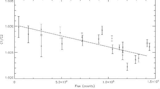
C1/C2 for the spectra of HD 189733 and HD 209458 for 10 different flux levels. The trend here is linear, indicating that the spectra become more tilted towards the red end of the spectrum for lower flux values. We note that WASP-12 is not included as the flux level remained relatively stable throughout the observing run, with only a handful of spectra varying due to short-term transparency variations. This was due to better weather conditions and more steady transparency.
From Fig. 2, it can be seen that at lower flux levels, the ratio is higher, meaning the spectra are essentially more sloped at lower overall flux values. The question now becomes what is the cause of this difference in the ratios of the continuum flux levels. Is it solely due to a non-linearity of the detector, or could there be some other underlying cause? Upon further investigation, we determined a possible cause could be atmospheric extinction – the effect of losses at a specific wavelength due to absorption/scattering by the Earth's atmosphere. This effect would manifest as a correlation of the ratio of C1 to C2 with airmass. Fig. 3 shows a linear correlation between the ratio and airmass, along with the trend modelled as a least-squares fit. This trend appears for all three objects, indicating that this is a systematic inherent to the observations as a whole.
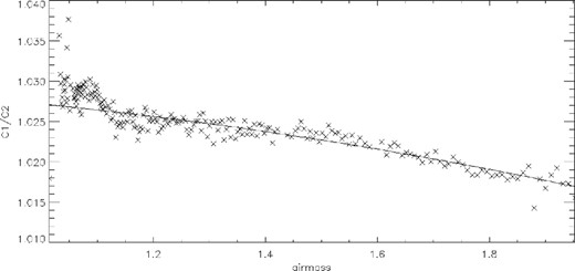
The ratio of C1 to C2 as a function of airmass for HD 189733. The trend here indicates that as the airmass increases, the continuum ratio decreases.
After this term was removed, we searched the corrected continuum for any correlations with parameters such as spatial position of the spectra on the CCD, FWHM, sky background, temperature of the chip and peak continuum count level. No correlations could be found for the out-of-transit data not affected by poor weather conditions. However, in order to fully characterize these systematics for this observing method, a data set observed under near-photometric conditions would be desirable in order to check for any additional correlations that may be present at a low level not identified in our current limited out-of-transit data set. We used identification and analysis of these systematics in these data sets to provide similar corrections to WASP-12 described in the next section.
5.2 WASP-12
In order to search for additional Na absorption in the WASP-12 data, we performed an analysis with molly to integrate the flux within predefined wavelength windows for two different regions – the Na doublet (5885–5900 Å) and the blueward comparison region of the continuum (5720–5860 Å) – after we had performed the correlation analysis on these data in the same manner as described in Section 5.1 (see Fig. A1). This matches the continuum windows used in the systematic analysis for HD 189733 and HD 209458. In order to attempt to detect a deepening of the Na lines relative to the surrounding continuum, we adopted a similar approach to Snellen et al. (2008). First, we normalized the spectra, and then performed the flux analysis using masks to integrate under different parts of the spectra. The final step, once all necessary correlations had been removed (as detailed in Sections 5.1), was to measure the ratio of the integrated flux in the two windows. This flux ratio should be constant (within error bars) throughout the night if we assume no Na absorption is taking place. However, if the lines do deepen due to the influence of the atmosphere of WASP-12b during transit, the integrated flux ratio will be different when comparing the in- and out-of-transit flux ratios. During our observations, we were able to achieve a SNR of 200 per spectrum.
Snellen et al. (2008) report that the detection of Na in the atmosphere of HD 208458b was significantly stronger when a narrow window was used. They used three different window sizes termed ‘narrow’, ‘medium’ and ‘wide’, that were positioned over each line in the Na doublet, with widths 0.75, 1.5 and 3.0 Å, respectively. The relative photometric dimming of the Na feature to the surrounding continuum were deeper by 0.056 ± 0.007 per cent (wide), 0.070 ± 0.011 per cent (medium) and 0.135 ± 0.017 per cent (narrow). In order to determine if Na could be detected in our WASP-12 data, we opted to use a single window which would maximize the contrast of the Na region relative to the continuum. A number of different window sizes were trialled during this analysis, and a 2.0 Å window over each component of the doublet was determined to be wide enough so as to avoid any issues such as clipping the Na line, but sufficiently narrow as to allow the contrast to be maximized. While this is wider than the ‘narrow’ and ‘medium’ windows used by Snellen et al. (2008), this was necessary due to the lower resolution of the ISIS data. Fig. 4 shows the masks used to analyse the Na doublet in the WASP-12 spectra, at 5889–5891 and 5894–5896 Å.
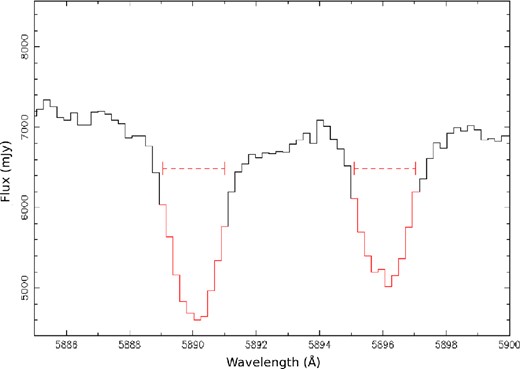
The mask used in the search for Na absorption. The regions used in the search are highlighted in red, and are 2 Å across.
A number of approaches were taken for comparing the Na and continuum windows. The analysis was carried out on spectra before normalization – in order to search for systematics – and post-normalization, after the correction for systematics had been made. The difference between the spectra post-normalization in both cases (i.e. with and without correction for airmass) is negligible, indicating that the normalization does indeed remove any trends which would adversely affect the search for additional Na absorption. Despite this, we opted to use the spectra which had the airmass term removed so that any subtle effects will have been removed prior to normalization. The final step before searching the Na region was to ensure that the normalization of the spectra were carried out successfully. Since the WASP-12 data were unaffected by variable cloud coverage, a simple two-term polynomial could be used in order to normalize the spectra. In order to ensure that the normalization process did not introduce any systematics, a thorough investigation into the normalized continuum region was carried out. This was done by examining the residuals present in the continuum after dividing the normalized spectra by the average out of transit spectrum. These residuals were explored to look for regions which showed evidence of systematic variation – something which may have been introduced by the normalization process. After performing this analysis, no such systematics were found, indicating that the normalized spectra could now be used to search for an Na absorption signature. Fig. 5 shows the continuum region residuals, in addition to the average out-of-transit spectra used to obtain these residuals. Note that the trail of the residuals appears featureless, indicating that the normalization process has not introduced any additional systematics.
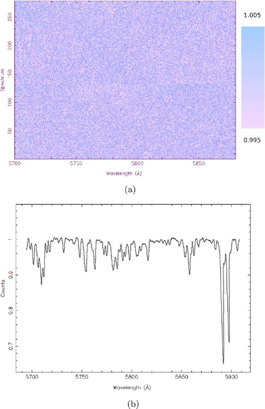
(a) Trail of the residuals after dividing the normalized spectra by the average out-of-transit WASP-12 spectrum. Very little variation appears in the residuals, as indicated by the colour bar. (b) The average WASP-12 out-of-transit spectra. Note that no systematics appear in the trailed spectra, indicating that the normalization has been performed correctly, and does not introduce additional sources of error.
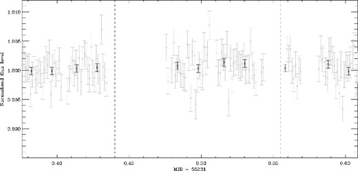
The data were then analysed using the Na mask, and the continuum region mask (5720–5860 Å) in order to generate two sets of normalized fluxes – the Na doublet and the blueward comparison continuum region. A number of different continuum masks were trialled, including masks of the same width and separation of the Na doublet region, in addition to masks spanning both sides of the Na feature. The mask we chose to use from this point on in the analysis gave a large enough coverage so as to ensure a sufficient comparison, but was also positioned sufficiently far from the Na region so as to avoid potential interference. Fig. 6 shows the ratio of the light under the Na mask to the continuum region. During transit, this ratio decreases, indicating that the Na lines are deepening. As the planet moves out-of-transit, the flux ratio increases back to its pre-ingress value. The second binned point in transit which appears at a similar level to the out-of-transit points occurs at the same time as a drop in the flux at mid-transit (see Fig. A1), thought to be due to transparency variations. The correlations of Na/continuum flux ratio with position, continuum flux, seeing and sky background were thoroughly investigated, and no trends could be found, either before or after normalization (see Fig. A2). Again, since this is based on only one night's data, low-level correlations may become apparent as more observations are made.
The Na region divided by the continuum for the normalized spectra over the first night of observation. The black points are the data after binning, and the grey points are the data prior to binning. The dashed lines indicate the times when the planet is in transit.
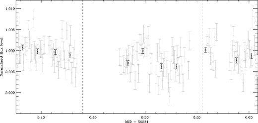
In addition, we also performed a check using the same Na mask on a number of featureless regions in the continuum. Since there should be no variation in the depth of the normalized continuum features, this analysis gives an excellent check to determine whether this deepening is unique to the Na region. Despite using the same mask widths, and using a large range of the continuum to perform this analysis, the decrease in flux ratio we see in the Na region does not occur anywhere else in the continuum. Fig. 7 is a similar plot to Fig. 6, but rather than centring on the Na doublet, the Na mask has been set to a featureless region of the continuum (5800–5810 Å). We also tested the window using regions away from the comparison region, on both sides of the Na doublet to ensure there was no variation in the ratio. Upon testing these regions, the ratio showed no such change as in Fig. 6.
A featureless region of the continuum from 5800–5810 Å has been analysed as opposed to the Na region. Again, the black points are the binned data and the grey points are the unbinned. Note that in this case, the points are almost constant, without the deepening seen in Fig. 6. This analysis was performed over a number of different regions in the spectra, and similarly, no deepening could be found (see Fig. 8).
The result of these tests is almost identical no matter where in the continuum the Na mask is placed. In Fig. 8, we show the difference between the in- and out-of-transit flux ratios for the windows that were chosen along the continuum, as well as when the window covers the Na region.
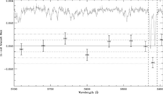
The difference in flux ratio (in-out of transit flux) for a series of windows in the comparison region for the Na feature (highlighted by the vertical dashed lines). The horizontal error bars represent the wavelength coverage of the mask in the spectrum analysis. The dot–dashed, dot–dot–dashed and dotted horizontal lines are the 1σ, 2σ and 3σ levels, respectively. The points have been overlaid on an example WASP-12 spectra for an indication of where the windows were placed. Note how the Na region is the only one which shows a significant difference between the in- and out-of-transit depths, lying in the 3σ region. The comparison windows have been taken at 30 Å intervals along the continuum.
We can therefore state that the increased absorption during transit is unique to the Na doublet for this data set. Whether this is an effect of the atmosphere of WASP-12b, or a still-unknown systematic only affecting the Na region (such as an issue caused by linearity) is still unknown, and will require further observations to fully confirm or deny any claim to the detection of the atmosphere. For example, changes in the stellar spectrum due to star spots could cause interference in the Na line depth. This could have the effect of either mimicking an Na detection from the exoplanet atmosphere, or interfering with the level of Na absorption during transit. The umbral region of a starspot on a G-type star covering a stellar surface area of 20 × 10−6A1/2⊙ has been shown to dilute the Na II line depth relative to the continuum region by 0.033 ± 0.05 per cent (Fay, Remo & Czaja 1972). This indicates that a particularly high level of stellar activity during observations could mimic the level of Na absorption found during previous transmission spectroscopy studies (e.g. this should be compared to the Na transit signature found for HD 209458b, 0.135 ± 0.017 per cent; Snellen et al. 2008). During previous observations however, WASP-12 has displayed low-levels of stellar activity (Haswell et al. 2012; Sing et al. 2013), indicating that any Na II deepening at the levels comparable to those found by Snellen et al. (2008) are unlikely to be solely due to sunspots. In addition, Na II deepening caused by stellar variability would not only affect the spectra during transit, and hence monitoring large portions of out-of-transit data would also provide a method to characterize short-period changes in the Na lines due to this effect.
One could also argue that the deepening around the Na doublet could be caused by tellurics, since our search is in the wavelength region where these lines start to become an issue (≳5885 Å). However, when we move our masks to continuum regions which should also be affected by tellurics – 5880–5887 Å and above 5900 Å – no additional deepening was detected when performing our flux ratio analysis. Placing masks in this region also has the additional advantage of checking for instrumental effects in the part of the spectrum near the edge of the CCD. We considered carrying out a similar telluric analysis to that performed by Snellen et al. (2008), where a synthetic telluric spectrum was constructed, matched to the resolution of the data, and monitored by comparison with a telluric standard. However, the slit width we used for our arc line acquisition made lines ‘top-hat’ shaped, meaning we are unable to accurately model the instrumental broadening profile of our spectra.
Another effect one must consider is that of limb-darkening. If the planet transits an optically thick part of the star, the continuum will deepen as compared to the Na line. Previous investigations have revealed that the effect of limb-darkening is minimal (Charbonneau et al. 2002; Snellen et al. 2008) when investigating the continuum surrounding the Na region. Our observations were also set-up to specifically avoid an unknown source of absorption redward of the Na doublet (as reported by Sing et al. 2008), which would have been significantly worse than the limb-darkening signal. Redfield et al. (2008) find the impact minimal, with excess limb darkening absorption contributing +1.46 × 10⁻⁵ to their Na signal of (−67.2 ± 20.7) × 10−5. The limb darkening for our measurements should fall well within the error on any detection of the Na absorption at the level of ∼0.005 per cent. Finally, the contribution of the companion objects to WASP-12 to the Na region must be considered. As mentioned in Section 1, WASP-12 is part of a triple system, meaning the companions to the WASP-12b host star may impact the Na measurements. Bechter et al. (2014) find the two objects to be M3V dwarfs, with a separation of 84.3 ± 0.6 mas. In order to investigate the specific effect of the M-dwarf pair on both the continuum region and the Na lines, we estimated the dilution factor in the wavelength range 5700–5920 Å. Assuming all three objects are at the same distance away (as found by Bechter et al. 2014), we obtained synthetic spectra for a G0 star and an M3V dwarf using the PHOENIX NextGen2 model atmosphere grid (Hauschildt et al. 1999). We matched the temperature, metallicity and log g values to the nearest observed values taking a cooler temperature for WASP-12 (since NextGen2 increases in 200k increments) so as not to underestimate the contribution. By comparing the synthetic spectra in this region, we estimate that the fractional contribution in the Na region by the M-dwarfs is negligible and in the nearby continuum region is 1.7 per cent for each M-dwarf in the system. Obtaining more observations of this system would allow for an opportunity to monitor the continuum region to see if the contribution is stable or changes over time. Any future defocused transmission spectroscopy observations which aim to detect planetary atmospheres around multiple-star systems should be mindful of this effect and attempt to estimate the fractional contribution of any companions.
If we are to assume that the deepening of the Na lines for the first night is due to the atmosphere of WASP-12b, we can obtain the corresponding sodium absorption. We obtain a value of 0.12 ± 0.03 per cent, a value which is very similar to the narrow absorption band of Snellen et al. 2008 for HD 209458b (0.135 ± 0.017 per cent). In order to check that this result is physically consistent with a real atmosphere detection, the data were analysed using wider masks. Increasing the size of the wavelength region being analysed has the effect of decreasing the effective Na cross-section, resulting in smaller absorption signals. This has been the case with most Na exoplanetary atmosphere detections (Charbonneau et al. 2002; Redfield et al. 2008; Snellen et al. 2008; Sing et al. 2008). Increasing the size of the wavelength mask surrounding the Na region also has the effect of analysing more of the redward and blueward regions, providing a further investigation into the surrounding Na features. The results of this are shown in Table 1.
Results of the analysis using masks of increasing size. Note that the error here has been adjusted to include uncertainty arising from the systematic spike present mid-transit.
| Mask width Å | Absorption signal per cent | Error per cent |
|---|---|---|
| 2 | 0.12 | 0.03 [+0.03] |
| 4 | 0.04 | 0.022 [+0.03] |
| 10 | 0.01 | 0.012 [+0.03] |
| Mask width Å | Absorption signal per cent | Error per cent |
|---|---|---|
| 2 | 0.12 | 0.03 [+0.03] |
| 4 | 0.04 | 0.022 [+0.03] |
| 10 | 0.01 | 0.012 [+0.03] |
The values we return for the 4 & 10 Å masks do indeed follow with what we expect, with the absorption signal decreasing for the wider masks. The 4 Å mask shows a lower absorption depth (0.04 ± 0.022) and the 10 Å mask shows no additional absorption (0.01 ± 0.012). However, whilst these results do show what one would expect, it is important to note that since this is still based on a single night's data, these absorption depths may be liable to systematics we are unable to account for, and therefore need further observations to check whether this is a real physical effect due to the atmosphere. We note that our figure also includes the rise in the ratio during the transit, thought to be due to the brightening sky background. This means our figure of 0.12 per cent is diluted by this systematic effect. We also note that 0.03 per cent is our formal error using the error from the data points, and will increase due to the systematic feature mid-transit. In order to characterize the effect of this systematic, the model light curve used to calculate our absorption depth was subtracted from the data. These residuals were binned (in the manner prescribed by Pont, Zucker & Queloz 2006), and the mid-transit systematic feature determined from this. Fig. 9 shows the result of this analysis using a binning factor of 6. As can be seen from this figure, the residuals at the mid-transit point are the only ones to show significant positive deviation from 0, indicating the region most affected by this unknown source of noise. Isolating this series of data and removing it from the absorption analysis give a new absorption depth of 0.15 ± 0.05 per cent, a difference of 0.03 per cent from the unaltered case. We have indicated the effect of this systematic on our Na absorption depth by indicating the additional systematic error alongside the statistical error, i.e. 0.12 ± 0.03[+0.03] per cent. This is a significant effect, and indicates the influence that systematics can have on a single data set. Whilst this is still a physically reasonable absorption signal, removing points has increased the error. This type of analysis should be employed during future observations to check if the data are similarly affected by such systematics at any point during the transit.
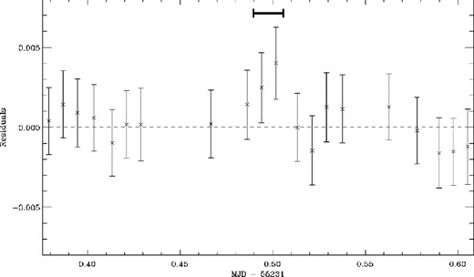
The residuals returned from the light-curve analysis using a binning factor of 6. This bin factor was determined using the method outlined in Pont et al. (2006). Note the points which rise mid-transit, causing the absorption depth to lower. We concentrated on analysis on these series of points (highlighted above with the bar range) to determine the potential error they introduced.
Since we expect the Na absorption of WASP-12b to be slightly higher than that of HD 209458b (due to the large scale height we are probing in addition to the extreme distortion and mass loss of the atmosphere), this seems a reasonable figure, given the systematic occurring mid-transit. In order to place further statistical significance on the Na detection, we opted to take a Monte Carlo approach. We selected a number of random out-of-transit spectra from our Na region, and used this in place of our in-transit selection. Carrying this out over 25 000 iterations gave excellent estimations of the false alarm statistics present in the data. This gave the 68 per cent, 95 per cent and 99.7 per cent bounds for our data, which are shown by the dotted and dot–dashed lines in Fig. 8. As can be seen, the Na point does lie within the 99.7 per cent population, indicating that the deepening of the lines is unlikely to be due to random error.
6 DEFOCUSED TRANSMISSION SPECTROSCOPY AS AN OBSERVING TECHNIQUE
An important aspect of the research carried out during these observations was investigating the technique of defocused transmission spectroscopy. Whilst the observations themselves were marred with poor weather conditions and technical issues, a number of issues were discovered which will enable future runs to be carried out much more efficiently. In addition to this, the initial exploration of the data has led to a potential detection of Na in the atmosphere of WASP-12b, indicating that the technique is feasible on telescopes the size of the WHT. Features such as the rise in flux ratio mid-transit also provide areas which could be investigated during future observations. Is this a real feature, or simply an unknown systematic? Our statistical analysis does indicate that it has a significant effect on the absorption depth. In regard to the technique of Defocused Transmission Spectroscopy, we have demonstrated that there does exist extensive justification for the refinement, development and continued use of the technique based on our data. Further observations will be able to improve upon both the technique and data analysis to make this a powerful method of observation for characterizing exoplanetary atmospheres.
7 FUTURE OBSERVATIONS
Our pilot study of defocused transmission spectroscopy revealed a number of improvements to the technique which could be easily applied to future observations. This section details some additional steps one should take during data acquisition and analysis to further improve the technique.
In order to fully characterize any potential contamination due to tellurics, it is desirable to follow the method prescribed by Snellen et al. (2008). In order to model the tellurics using a synthetic telluric spectrum, the line-list needs to be convolved with the instrumental broadening profile. While this could be obtained from the arc lines, the arc frames during our observations were taken with a wide slit, meaning the arc lines appear as ‘top-hats’ and hence the profile could not be accurately obtained. Fig. 10 shows how tellurics would be modelled if it were possible to convolve the line-list with the instrumental broadening profile for the data. The top (blue) spectrum is a synthetic telluric spectrum from Lundstrom et al. (1991), along with a WASP-12 spectrum centred on the Na doublet.
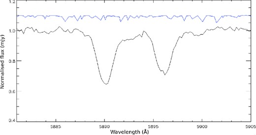
The region where we expect telluric contamination to potentially deepen the lines. The top blue line is a synthetic telluric spectrum created from the line lists of Lundstrom et al. (1991). The bottom plot is a WASP-12 spectrum showing the Na doublet. Note how the telluric features will affect both the Na lines themselves and the continuum surrounding these lines. We note here that due to the resolution of the synthetic spectra, the lines are only representative of their position, not necessarily their depth.
It would also be desirable to obtain a data set of a bright target (e.g. HD 189733) under photometric conditions, with ample out-of-transit data. This would allow for the systematics of the technique to be further investigated and characterized. Such a data set could allow for additional systematics (such as instrumental effects) to be modelled by injecting a fake transit into the spectra, and attempting to recover the signal. Such techniques would provide a useful investigation into additional methods of attempting to detect absorption due to an exoplanet atmosphere.
When observing the transit, future observations should aim to get as much out of transit data as possible in order for any potential sodium detection to have a large number of continuum regions to compare to. For our initial observing run, we were limited to two half nights, due to the position of the object on the sky. Observations of the full transit and ample out-of-transit spectra would allow for any trends in the Na/continuum flux ratio to be monitored both prior to ingress and post-egress. It would also be useful to obtain a data set of in-focus transmission spectroscopy observations using the same instrumental set-up. This would provide a direct comparison between the techniques, and would give an indication as to the improvement defocusing has on observations. In addition, better characterization of the linearity of the CCD would allow for an explicit separation of airmass correction and linearity correction during data analysis.
The C1/C2 correction was applied by removing the trend in the comparison region of the spectrum, extrapolating this to the whole spectrum prior to normalization. Doing this does ensure a better comparison region; however, extrapolating towards the Na region is not ideal, as there may be some residual curvature in the spectrum which this method does not take into account. In order to provide a thorough check of all parts of the spectrum, future observations should aim to obtain coverage redwards of the Na doublet which can be compared with the blueward spectrum to fully investigate any curvature in the spectrum prior to correction. Whilst this region may be prone to an unknown source of absorption, it does not have to be used in the Na/continuum analysis, and provides an additional investigation of the systematics.
8 CONCLUSIONS
The technique of defocused transmission spectroscopy has the capacity to allow for the characterization of exoplanet atmospheres of fainter targets, providing observational constraints to atmospheric models. Any tentative detection of Na in the atmosphere of WASP-12b is a significant result, providing a potential insight into this highly irradiated, highly inflated hot-Jupiter. This detection would also provide a direct observational test of the pM/pL classification system. Not only should Na not be detectable, due to TiO/VO swamping Na at these wavelengths, but the level we detect it at indicates that WASP-12b should fall into the pL category. This runs directly contrary to the predictions made by Fortney et al. (2008) for such an irradiated system, and provides evidence that the classification scheme may need reappraisal. Recent observations by Sing et al. (2013) also indicate the need for reappraisal due to the lack of TiO in the atmosphere of WASP-12b. In addition, constraints on the PT profile of the atmospheres of hot-Jupiters can be obtained from measurements of Na, giving further evidence for or against the predictions of atmospheric models. Recent HST Wide Field Camera 3 (WFC3) WASP-19b transmission spectroscopy observations find a lack of TiO absorption features, and a signature of H2O in the atmosphere (Huitson et al. 2013). WASP-19b, like WASP-12b, is predicted to lie in the pM region of the classification scheme of Fortney et al. (2008) and should, therefore, be dominated by TiO absorption. The claim of Huitson et al. (2013) that TiO is reduced in the atmosphere of WASP-19b runs contrary to the predictions of the pM/pL classification scheme, much like the WASP-12b Na detection presented in this paper. Both of these results provide an indication that the classification system should be reconsidered. Further transmission spectroscopy measurements will allow for more observational points to revise this, or indeed any, classification scheme.
From the extensive analysis of systematics and correlations for the data, a number of preliminary areas for investigation as to how to characterize and monitor systematic variations during future observations have been identified. The effects of both short- and long-term variations during observing have been noted, in addition to investigating correlations between the flux and available parameters. However, due to poor weather conditions and the low resolution of the data, further observations must be made in order to obtain a better understanding of how systematics such as telluric contamination and linearity of the detector affect the fully reduced spectra. We have eliminated a number of potential causes which could mimic the Na absorption effect during transit, and investigated other potential causes, such as deepening due to telluric contamination and linearity. While there does not appear to be any evidence of these systematics, more data at a higher resolution are desirable in order to fully eliminate these.
Overall, the detection of Na at the level presented in this analysis is potentially a very significant result. Based on a single night's data, there does appear to be a possible detection of additional Na absorption due to the atmosphere of WASP-12b. However, more observations are required before such a detection is confirmed. Nonetheless, the technique of defocused transmission spectroscopy does appear to be a viable method for the detection and characterization of exoplanet atmospheres. Further use of the technique will allow for it to be refined to make direct detections from ground-based platforms.
The authors gratefully acknowledge the use of Tom Marsh's software packages molly and pamela. JB was funded by the Northern Ireland Department of Employment and learning. CAW acknowledges support from STFC grant ST/L000709/1. PRG is supported by a Ramón y Cajal fellowship (RYC–2010–05762), and also acknowledges support provided by the Spanish MINECO under grant AYA2012–38700. The WHT is operated on the island of La Palma by the Isaac Newton Group in the Spanish Observatorio del Roque de los Muchachos of the Instituto de Astrofsica de Canarias. We would especially like to thank the referee for numerous helpful comments after initial submission of this work.
REFERENCES
APPENDIX
Observations of the three candidates in our pilot study. Note that switching the observing mode from ‘fast’ to ‘slow’ was due to an issue with the CCD controller.
| Target | Transit | Slit width (arcsec) | Flat-fields | Exposures | MJD start | Exp time (s) | Read mode | Observing Conditions |
|---|---|---|---|---|---|---|---|---|
| WASP-12 | In-transit | 2.48 | 1055 | 53 | 55231.476 | 101 | Fast | Some light cloud |
| Out-transit | 79 | 55231.376 | 101 | Fast | Some light cloud, mostly clear | |||
| In-transit | 2.48 | 1004 | 48 | 55232.526 | 101 | Fast | Some light cloud, mostly clear | |
| Out-transit | 98 | 55232.396 | 101 | Fast | Mostly clear | |||
| HD 209458 | In-transit | 2.48 | 2226 | 96 | 55445.452 | 51 | Slow | Light cloud |
| Out-transit | 202 | 55445.373 | 51 | Slow | Cloudy | |||
| HD 189733 | In-transit | 2.48 | 1205 | 239 | 55446.367 | 51 | Slow | Variable cloud |
| Out-transit | 52 | 55446.359 | 51 | Slow | Light cloud |
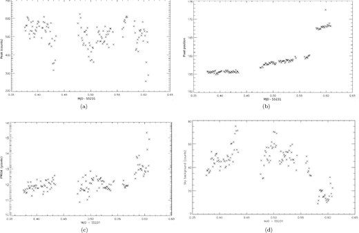
WASP-12 analysis – MJD versus (a) continuum flux. (b) Position of spectra on the CCD. (c) FWHM. (d) Sky.
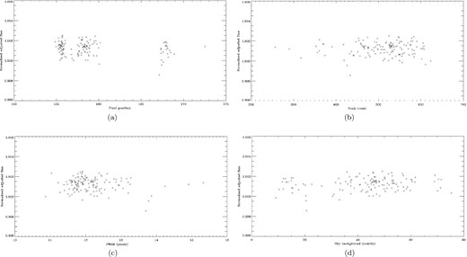
Night 1 correlations, normalized, corrected flux versus (a) position. (b) Continuum flux. (c) FWHM. (d) Sky background. Note how there appear to be no correlations post normalization, given the variability of the parameters in Fig. A1.
