


Abstract
Strong downstream magnetic fields of the order of ∼1 G, with large correlation lengths, are believed to cause the large synchrotron emission at the afterglow phase of gamma-ray bursts (GRBs). Despite the recent theoretical efforts, models have failed to fully explain the amplification of the magnetic field, particularly in a matter-dominated scenario. We revisit the problem by considering the synchrotron emission to occur at the expanding shock front of a weakly magnetized relativistic jet over a magnetized surrounding medium. Analytical estimates and a number of high-resolution 2D relativistic magnetohydrodynamical (RMHD) simulations are provided. Jet opening angles of θ = 0°–20°, and ambient to jet density ratios of 10−4–102 were considered. We found that most of the amplification is due to compression of the ambient magnetic field at the contact discontinuity between the reverse and forward shocks at the jet head, with substantial pile-up of the magnetic field lines as the jet propagates sweeping the ambient field lines. The pile-up is maximum for θ → 0, decreasing with θ, but larger than in the spherical blast problem. Values obtained for certain models are able to explain the observed intensities. The maximum correlation lengths found for such strong fields is of lcorr ≤ 1014 cm, 2–6 orders of magnitude larger than the found in previous works.
1 INTRODUCTION
Gamma-ray bursts (GRBs) liberate a significant fraction of the rest-mass energy of their source (>1051 erg) over intervals ranging from a fraction of a second to minutes. The standard fireball picture (Paczyński 1986; Shemi & Piran 1990; Rees & Meszaros 1992; Sari, Narayan & Piran 1996) explains the otherwise puzzling ability of such sources to vary on short time-scales by arguing that the bursts are produced via a relativistic outflow with a bulk Lorentz factor Γ > 100. At first, the relativistic flow is dissipated internally [via internal shocks (IS) or via another form of internal dissipation, like magnetic instabilities] that produce the prompt γ-rays. Later the interaction of the flow with the circum-burst matter produces an external shock and this blast wave produces the subsequent afterglow at lower frequencies. Observational clues concerning GRB progenitors indicate that supernova explosions of massive stars could be the predominant sources of long GRBs (i.e. those whose gamma emission lasts more than 2 s and the standard model for these objects is the Collapsar model; Woosley 1993; Paczyński 1998; MacFadyen & Woosley 1999). The main possible sources of short GRBs are mergers of neutron stars (NSs) with other NSs, or with black holes (Eichler & Cheng 1989), although other driving sources such as phase transition of a NS to a quark star have also been proposed (Lugones et al. 2002).
The field of GRBs has rapidly advanced in recent years, especially following the launches of NASA missions Swift and Fermi, both in the past decade. Due to their elusive nature, observing GRBs in all wavelengths at all epochs (including during and after the GRB) is still challenging with the current GRB detectors and follow up telescopes. As a result, for every new temporal or spectral window unveiled a rich trove of new phenomenology is uncovered (Zhang 2011). The new observations have raised new questions.
The composition of the relativistic jets that arise in GRBs is uncertain due to the lack of direct observations. The most important unknown parameter is the ratio (σ) between the Poynting flux and the matter flux (here both baryons and leptons are considered). In the standard fireball IS scenario, magnetic fields are assumed not to play dynamically any major role, i.e. σ ≪ 1. An alternative view is that the GRB outflow is powered by magnetic extraction from the rotational energy of a massive star or an accreting black hole and therefore, carries a dynamically important magnetic field component, i.e. σ ≫ 1. The GRB radiation in this case would be powered by dissipation of the magnetic field energy in the ejecta (e.g. Usov 1992; Thompson 1994; Meszaros & Rees 1997; Piran 1999, 2005; Lyutikov, Pariev & Blandford 2003; Zhang & Yan 2011). Even in a matter-dominated outflow where the magnetic field does not influence the dynamics, magnetic fields play a crucial role at the radiation emission region. Magnetic fields dominate the process of particle acceleration in the collisionless shocks and also play an important role on the afterglow synchrotron emission.
Another important aspect related to magnetically dominated (large σ) jets is that observations require that they become matter dominated at some point beyond the central engine, with the conversion of the energy transported outward in the form of Poynting flux into kinetic energy flux. The mechanism by which this occurs is not known yet. It could be related to gradual acceleration of the flow (Heyvaerts & Norman 1989; Chiueh, Li & Begelman 1991; Bogovalov 1996; Lyubarsky 2009), or to impulsive acceleration (Granot, Komissarov & Spitkovsky 2011; Granot 2012), or even to non-ideal MHD effects such as magnetic reconnection (Lyutikov et al. 2003; Giannios & Spruit 2006; Lyubarsky 2010; Zhang & Yan 2011; McKinney & Uzdensky 2012; Levinson & Begelman 2013), or magnetic kink instabilities (Giannios & Spruit 2006; Levinson & Begelman 2013). This has been known as the σ problem and more recent analytical and numerical studies suggest that this conversion may occur even before the jet breaks out from the stellar envelope (Levinson & Begelman 2013; Bromberg et al. 2014; Beniamini & Piran 2014).
The ejecta can be parametrized by ϵB and ϵe which give the ratios of magnetic and kinetic energies with respect to the total energy density of the ejecta, respectively. Typical values derived from the synchrotron emission assuming approximately energy equipartition between the relativistic electrons and the magnetic field range from ϵB = 10−5 to 10−2 (Waxman 1997; Galama et al. 1999; Yost et al. 2003; Li & Zhao 2011; Santana, Barniol Duran & Kumar 2014). In general, both parameters are assumed to remain constant in the afterglow region.
In the extreme case mentioned above that the magnetically dominated flow dissipates most of its magnetic energy before the breakout of the stellar envelope (Beniamini & Piran 2014; Bromberg et al. 2014), no significant magnetic field from the source will be carried out by the external shock that produces the afterglow emission. This implies that only the ambient magnetic fields swept and compressed by the ejecta will be available to accelerate the relativistic particles responsible for the synchrotron radiation.
On the other hand, even assuming that the ejecta drags most of the magnetic field from the source, Medvedev & Loeb (1999) considered the magnetic field of a strongly magnetized compact object with B ∼ 1016 G and found that it cannot account for the magnetic fields observed in the afterglow. The average field intensity over the emitting region scales as |$\bar{B} \propto r^{-2}$|. Therefore, one expects B ∼ 10−4 G and ϵB ∼ 10−7 at the afterglow emission, about 1016 cm away from the source.
Other mechanisms were proposed in the literature in order to explain the origin of the magnetic field in the afterglows of GRBs in a matter-dominated scenario. Most of them based on the growth of non-linear instabilities, such as the Weibel instability (Medvedev & Loeb 1999; Hededal et al. 2004; Nishikawa et al. 2005). This instability has its origin in the shock of two different populations of collisionless plasma particles. The diffusion of part of the populations into each other generates an anisotropy in the momentum distribution. The magnetic field amplification arises in order to isotropize the momentum distribution (Medvedev & Loeb 1999). Small fluctuations of the magnetic field deflect the particles by the Lorentz force leading to the generation of currents and the magnetic field increases. The deflections become stronger as the magnetic field increases generating a runaway process. In such instability, however, the amplified magnetic field is randomly oriented at very short correlation lengths (>δ), where δ is the plasma skin depth δ = c/ωp (ωp is the plasma frequency), in spite of the observed correlation lengths lcorr ∼ 1010 δ (Waxman 2006). Particle-in-cell (PIC) simulations have been performed in order to study this problem. For instance, Kazimura et al. (1998) found that about 5 per cent of the flow kinetic energy is converted into magnetic energy. Also, as pointed above, Nishikawa et al. (2003, 2005) showed that the Weibel instability amplifies non-uniform small-scale magnetic fields only. This could give origin to a jitter spectra instead of a Synchrotron radiation. Frederiksen et al. (2004) and Hededal et al. (2004) showed that the magnetic field amplitudes necessary to accelerate particles could be provided by this instability even in the case of a very weak upstream magnetic field, but these fields would still be small-scale ones. It is quite clear that such small-scale process is unable to provide the large-scale and strong magnetic fields as needed to explain the afterglow emission.
As stressed before, in a matter-dominated scenario, we are left with the ambient magnetic fields. The magnetic energy density increases due to the shock compression of the interstellar medium (ISM), which can be derived analytically from the one-dimensional relativistic Rankine–Hugoniot (RH). For an adiabatic shock, the RH relations predict amplification factors of ∼Γ, Γ being the Lorentz factor (Kennel & Coroniti 1984; Appl & Camenzind 1988; Summerlin & Baring 2012). Typical magnetic fields in the ISM of a few μG imply ϵB ∼ 10−11 (Medvedev & Loeb 1999). However, when considering the confinement of the magnetized expanding flow between the forward bow shock and the reverse shock the amplification of the magnetic fields is more efficient, as also qualitatively evidenced in former numerical studies of non-relativistic and relativistic jets (e.g. Leismann et al. 2005). A systematic study of the magnetic field evolution and amplification in such systems, sweeping a vast parametric space, is still missing though.
In this work, we revisit the problem of the magnetic field amplification behind the shocks of GRBs. The paradigm considered here for the afterglow emission is that described e.g. in Granot & Konigl (2001):
In the case of GRB afterglows, the most common interpretation is in terms of shocks that form at the interface between the relativistically outflowing material and the surrounding medium (with the bulk of the observed emission arising in the ‘forward’ shock that propagates into the ambient medium...). The radiation is inferred to be non-thermal, with the dominant emission mechanisms most commonly invoked being synchrotron and inverse Compton.
In this context, we study numerically the time evolution of the magnetization in the shocks generated by a relativistic jet. We adopt the matter-dominated outflow scenario and explore the amplification of ambient magnetic fields at the shocks by means of two-dimensional (2D) relativistic magnetohydrodynamics (RMHD) numerical simulations. Our goal is to study whether the resulting compressed fields behind the shocks are sufficient to explain the observed afterglow emission without requiring a magnetically dominated flow scenario.
We study different possible scenarios. Specifically, we consider the expansion of conical jets with different opening angles, from θ = 0 (cylindrical case) up to 20°, before and after they break out from the stellar envelope expanding over the interstellar gas with either smaller or larger densities than the later.
The paper is organized as follows. In Section 2 we review the basic jump conditions in RMHD shocks. In Section 3 we describe the numerical setup and the RMHD equations to be solved numerically in two-dimensions (2D). In Section 4 we describe the numerical results from the simulations and show the magnetic field amplification due to shock compression and pile-up behind the shocks at the jet head. In Section 5 we study the coherence length of the magnetic field using structure functions (SFs) and compare them with other proposed mechanisms of magnetic field amplification. Finally, in Section 6, we discuss our results and the implications for GRB jets and draw our conclusions.
2 RELATIVISTIC SHOCKS
According to the conservation equations above, the amplification of the magnetic field occurs due to the strong shock compression. The basic assumption of a fluid frozen into the magnetic fields results in an equal jump condition for both ρ and B. Therefore, for strong shocks, part of the kinetic energy is converted to magnetic energy.
This scenario is more complex if the shocked region is bounded by two shocks. Actually, this is the case of the high-speed jet propagating over the ambient medium. At the reference frame of a supersonic shock there are two incoming flows, the relativistic jet from one side and the ambient gas from the other with a contact discontinuity between them, where the kinetic linear momenta are equal. If compression leads to significant lateral expansion an outflow is expected to emerge in the direction perpendicular to the inflows (see Fig. 1), and this problem cannot be solved in one dimension.

Idealized and simplified picture of the shock fronts generated by a relativistic jet expanding over the ambient medium at rest. Differently to what happens in an isotropically expanding blast wave, the downstream ambient material is able to flow along the contact discontinuity. This results in a lower downstream pressure and in a thinner shock front, compared to the isotropic case.
Following Fig. 1, the upstream jet gas is decelerated at the shock discontinuity on the left (shock 1) and its downstream shocked material is pushed outwards in the lateral direction. The ambient material is shocked at the discontinuity on the right (shock 2), enters the shock region, and leaves outward, as well. The equilibrium of momentum between both downstream flows occurs at the contact discontinuity, and turbulent mixing of the fluids at this surface may occur.
Earlier three-dimensional (3D) numerical studies of hydrodynamical non-relativistic jets (Chernin et al. 1994) have demonstrated that this mixing depends mainly on the jet Mach number and the density ratio between the jet and the ambient gas. For small values of both parameters (Mach numbers <6 and density ratios <3) turbulent mixing and entrainment become important – a condition typically fulfilled, e.g. by certain classes of AGN jets (see e.g. de Gouveia Dal Pino & Benz 1993; Raga & Cabrit 1993; Stone & Norman 1993; de Gouveia dal Pino 2005, and references therein) and for further hydrodynamical studies (Folini & Walder 2000, 2006) (check also Cerqueira, de Gouveia Dal Pino & Herant 1997; Falceta-Gonçalves & Abraham 2012, for similar studies in non-relativistic MHD flows).
These authors also showed that the momentum transfer and width of the shocked region are strongly affected by the thermal radiative cooling of the shocked material. Strong cooling decreases the turbulent mixing (as part of the internal energy of the shocked material is radiated away) and also shrinks the shock region, as the downstream internal energy is small compared to the upstream kinetic one. A consequence of non-uniform cooling and thin shock regions is the growth of the non-linear thin layer instability (Vishniac 1994) and the Rayleigh–Taylor instability which can break the bow shock region into a healthy clumpy structure (Blondin, Fryxell & Konigl 1990; de Gouveia Dal Pino & Benz 1993, 1994; Stone & Norman 1993).
In the case of magnetized shock-bounded slabs, the upstream gas drags field lines into the shocked region. Depending on the orientation of the upstream fields, the downstream magnetic field lines are not carried away with the outflow. 2D MHD numerical simulations of non-relativistic converging flows reveal that part of the magnetic field component perpendicular to the shock velocity B⊥ is not advected, instead, it piles up and remains parallel to the contact discontinuity surface (Falceta-Gonçalves & Abraham 2012; Falceta-Gonçalves & Monteiro 2014). Then, the downstream shocked plasma flows along the amplified field lines outwards to fill the cocoon surrounding the jet beam. Since the jet is continuously pushing the ambient gas forward there is a constant inflow of ambient magnetic field lines into the bow shock region, causing the piling-up effect.
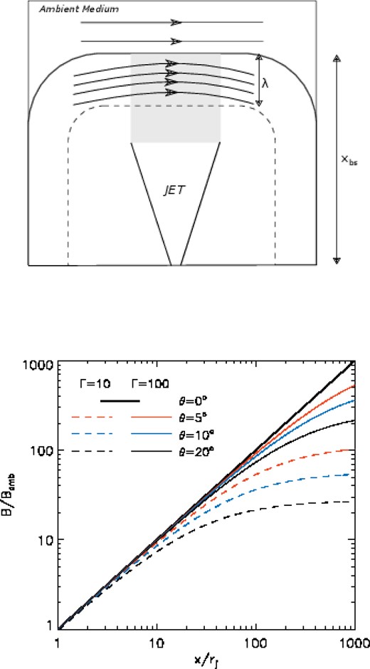
Up: schematic representation of the pile-up effect of the magnetic field lines as the jet propagates in an ambient medium with uniform magnetic field. Bottom: pile-up effect on the magnetic field intensity at the shock region for collimated and wide jets as a function of the distance, as given by equations (7) and (11), respectively, for different jet opening angles, and for Γ = 10 (dashed) and Γ = 100 (solid).
An analytical estimate of λ is not trivial though, mostly because of the asymmetric morphology of the shock region. The shock thickness for spherical relativistic blast waves has been derived as λ ∼ R/Γ (Blandford & McKee 1976), R being the shock wave radius. Since R = R(t), the thickness λ is also a function of time. This expansion of λ with time may be understood from the conservation of matter and energy. The shock dynamics is that of a one-dimensional radial Riemann problem, but with a uniformly expanding shocked volume as the shell expands. The accumulation, as the blast wave moves, results in local increase of enthalpy that leads to an expansion of the shock thickness.
As discussed later on in the paper, there are observational evidences – as well as results from numerical simulations – indicating that core-collapse GRB jets may be, in reality, not well collimated after the breakout of the stellar envelope. Observationally, power-law break decay during the afterglow emission has been well modelled by means of conical jets, with opening angles as large as 20°, being θj < 10° in a vast majority of objects (see Sari, Piran & Halpern 1999; Bloom, Frail & Kulkarni 2003; Frail et al 2001; Zeh, Klose & Kann 2006; Tchekhovskoy, McKinney & Narayan 2009; Bromberg et al. 2011; Mizuta & Ioka 2013).
Therefore, the pile-up must occur at shorter distances in the case of conical jets, with a departure from the linear growth of B and eventual saturation of the magnetic field amplification, consistent with causality constraints.
Using equations (7) and (11), we computed the pile-up effect which is shown in Fig. 2 (bottom) as a function of the distance to the central source, for different jet parameters. We clearly see in the figure that for large values of Γ, the difference between collimated (θ → 0) and wide jets decreases substantially.
As stated before, despite the extensive numerical multidimensional study that can be found in the literature of magnetized relativistic jet flows, a systematic study of the amplification of ambient magnetic fields by relativistic jets, particularly in the context of GRBs, is still missing. In the following sections we will explore this issue and test the scenarios above considering RMHD numerical simulations of both collimated and wide jets propagating over a weakly magnetized ambient.
3 GOVERNING EQUATIONS AND NUMERICAL SETUP
The above set of equations was solved using the godunov code (check http://amuncode.org for the public available source code) which implements the Godunov-framework of the hyperbolic equation numerical solution (Godunov 1959) extended by methods suitable to solve the SRMHD equations. The code has been extensively tested and applied to several astrophysical problems (e.g. Kowal & Lazarian 2010; Falceta-Gonçalves et al. 2010a,b; Falceta-Gonçalves, Lazarian & Houde 2010c; Santos-Lima et al. 2010; Kowal, de Gouveia Dal Pino & Lazarian 2011a, 2012; Kowal, Falceta-Gonçalves & Lazarian 2011b; Santos-Lima, de Gouveia Dal Pino & Lazarian 2012, 2013; Poidevin et al. 2013; Ruiz et al. 2013). In the work presented here we used the fifth-order monotonicity-preserving (MP) reconstruction (Suresh & Huynh 1997; He et al. 2011) of the Riemann states, the approximate HLLC Riemann solver (Mignone & Bodo 2006) in order to calculate the numerical approximation of the fluxes |${\bf F}$|. The solution advances in time using the third-order four-stage explicit optimal Strong Stability Preserving Runge–Kutta SSPRK (4,3) method (Ruuth 2006). In order to keep the divergence of magnetic field minimum, we use the hyperbolic divergence cleaning approach by Dedner et al. (2002).
A non-straightforward element of the solution of the RMHD equations is the determination of the primitive variables |${\bf Q} = (\rho , {\bf v}, {\bf B}, p)$| from their conservative representation |${\bf U}$| (see equation 13). While in the non-relativistic case the conversion requires only simple algebraic manipulations, here we are forced to use iterative methods. A number of such methods have been compared in Noble et al. (2006) with the conclusion that their 1Dw scheme is the most accurate and robust one and therefore, it is also employed in our calculations.
3.1 Initial setup
Significant progress has been achieved in the past years regarding relativistic jet simulations both in the framework of extragalactic jets (Marti et al. 1997; Aloy et al. 1999; Hughes, Miller & Duncan 2002) and of GRB jets (Komissarov 1999; MacFadyen, Woosley & Heger 2001; Zhang, Woosley & MacFadyen 2003; Leismann et al. 2005; Morsony, Lazzati & Begelman 2007; Tchekhovskoy, McKinney & Narayan 2008; Lazzati, Morsony & Begelman 2009; Mizuta & Aloy 2009; Tchekhovskoy, Narayan & McKinney 2010; De Colle et al. 2012; Mizuta & Ioka 2013; Bromberg et al. 2014), most of which were performed in the low σ regime and, due to computational limitations, in two-dimensions,2 but none focused on the investigation of the interaction of the shocks of the ejecta with the ambient magnetic field after the breakout of the collapsing stellar envelope.
There is some debate in the literature regarding the GRB jet opening angle at the breakout (see e.g. Lazzati & Begelman 2005; Morsony et al. 2007; Tchekhovskoy et al. 2008; Mizuta & Ioka 2013; Bromberg et al. 2014, and references therein). When inside the stellar envelope, collimation of a Poynting flux-driven jet may occur due to net currents driven locally, as well as by the surrounding pressure. The energy dissipation at the jet shock head increases the total pressure of a hot cocoon that develops around the jet which helps collimating the jet. Once the jet breaks out of the stellar envelope, it may become wider due to reduced pressure (Bromberg et al. 2011; Mizuta & Ioka 2013). There is in fact evidence in favour of conical jets. Tchekhovskoy et al. (2009), for instance, find from his simulations Lorentz factors Γ ∼ 100–5000 and opening angles θj ∼ 0.1–10°, reproducing inferred properties of GRB jets. On the other hand, the confinement inside the envelope of a Poynting flux-dominated jet due to both magnetic and cocoon pressure can be so large that the jet can emerge from the stellar envelope with a radius of the order of the source light cylinder radius (RL) and likely remain confined well after the breakout providing a consistent jet scenario for both the prompt gamma emission and the formation of a photosphere (Levinson & Begelman 2013).
Observationally, the opening angle is inferred by fitting the break in the power-law decay of the afterglow emission with the fluxes expected from an emitting plasma subject to relativistic beaming (Rhoads 1999). The fit model depends on several simplifications, such as the density distribution of the surrounding medium (e.g. for winds or ISM), and radial dependencies within the jet. Under these conditions, the vast majority of GRBs data results in θj < 10°, with fiducial estimates at θj ∼ 4° (Sari et al. 1999; Frail et al 2001; Bloom et al. 2003; Zeh et al. 2006).
While this question of the jet opening angle is still debatable (e.g. Lazzati & Begelman 2005; Morsony et al. 2007; Tchekhovskoy et al. 2009; Bromberg et al. 2014), in this work we explore different possible values for this parameter. At the inlet of the computational domain we start with a jet that has just emerged from the collapsing stellar envelope into the ambient medium. For the sake of simplicity the jet in our simulations is not launched from first principles, but injected as boundary condition. The opening angle is therefore a free parameter and in our simulations three conditions have been tested for it, namely θj = 0°,10° and 20°. Also, θj is set as constant as the jet emerges from the collapsing stellar envelope into the ambient medium.
The initial setup of the jet beam is built with a region of continuous injection of material into the computational domain of radius Rj, which defines the jet radius, set at the left vertical boundary of the box domain. The bottom horizontal and the left vertical boundaries of the box are assumed to be reflective, while the other are open boundaries allowing the material to leave the domain.
The ambient gas density ρ and pressure p are assumed initially uniform in the whole domain. Since we are interested in the study of the amplification of the magnetic field in the shock region of a matter-dominated flow, we set a weak uniform ambient magnetic field initially perpendicular to the propagation of the jet, corresponding to Pmag/Pth = 10−5.
Another important parameter for the dynamical evolution of jets, though not critical for the purpose of this work as we discuss further below in the paper, is the ratio between the surrounding ambient and the jet densities (η = ρamb/ρjet). Traditionally, relativistic jet propagation models for microquasars, AGNs and GRBs assume an underdense relativistic flow, i.e. with a density smaller than that of the ambient medium. One of the justifications for this assumption is the general absence of thermal emission in the shocks of these jets. In the collapsar scenario, if the GRB jet is magnetically driven, the launch occurs probably with η > 1 (see e.g. simulations by López-Cámara et al. 2013), as predicted by the semianalytical models and numerical simulations referenced in the previous sections. After breaking out of the envelope, far from the stellar material, the jet may change its mass regime and the jet density may become larger than that of the ambient, i.e. η ≪ 1. This is discussed, for instance, by Lazzati & Begelman (2005) and Morsony et al. (2007). Simulations of the jet–envelope interaction indicate a transition between the regimes of η ≃ 104–105 (at the central region of the stellar envelope) and η < 10−6 after the jet breaks the outer boundary of the star.
Since the dynamical evolution of the jet over a uniform ambient medium may differ considerably depending on the parameter η chosen, for the sake of completeness, we studied the dynamical evolution of jets in both regimes, i.e. η < 1.0 and η > 1.0, sweeping a parametric range 10−4 ≤ η ≤ 102. In this sense, we can study the different morphologies and magnetic field amplification for the phases of the jet interacting with the surrounding media right after the breakout of the stellar envelope and further out.
The space of parameters investigated in this work is presented in Table 1. In all cases the jet is initially relativistic (with Lorentz factors Γ = 2, 10, or 100) and supersonic, i.e. the initial Mach number, defined as M ≡ vjet/cs is set as 10 for all models, where the sound speed is given by |$c_{\rm s}=\sqrt{ \gamma \left(\gamma -1\right) P / \left[\left(\gamma -1\right)\rho + \gamma P \right] }$|.
Parameters used in each simulation run. We explore the dependence with the density ratio, polytropic index, Lorentz factor and opening angle. The angle equal to 0° refers to the case where the jet is injected with a cylindrical geometry.
| γ | Mach | Γ | ρamb/ρjet | θj | Model |
|---|---|---|---|---|---|
| 1.1 | 10 | 2 | 102 | 0° | NA1cyl |
| 1.1 | 10 | 10 | 102 | 0° | NA2cyl |
| 1.1 | 10 | 100 | 102 | 0° | NA3cyl |
| 1.33 | 10 | 2 | 102 | 0° | AD1cyl |
| 1.33 | 10 | 10 | 102 | 0° | AD2cyl |
| 1.33 | 10 | 100 | 102 | 0° | AD3cyl |
| 1.33 | 10 | 10 | 10 | 0° | AD4cyl |
| 1.33 | 10 | 10 | 1 | 0° | AD5cyl |
| 1.33 | 10 | 10 | 10−4 | 0° | AD6cyl |
| 1.33 | 10 | 10 | 10−2 | 0° | AD7cyl |
| 1.33 | 10 | 10 | 10−3 | 0° | AD8cyl |
| 1.33 | 10 | 100 | 10−4 | 0° | AD9cyl |
| 1.1 | 10 | 10 | 102 | 10° | NA1con |
| 1.1 | 10 | 100 | 102 | 10° | NA2con |
| 1.33 | 10 | 10 | 102 | 10° | AD1con |
| 1.33 | 10 | 100 | 102 | 10° | AD2con |
| 1.33 | 10 | 10 | 10−4 | 10° | AD3con |
| 1.33 | 10 | 100 | 10−4 | 10° | AD4con |
| 1.33 | 10 | 10 | 10−4 | 20° | AD5con |
| 1.33 | 10 | 100 | 10−4 | 20° | AD6con |
The dimensions of the simulated computational box is (Lx, Ly) = (48, 12) in code units. The adopted code unit for the distance is 5Rj. The code unit for time is defined as 5Rj/c, where c is equal to 1 in our simulations. The simulations were performed with a resolution of 4096 × 1024 cells.
The thermal radiative cooling of the hot shocked ambient plasma may result in thin and unstable shock regions. However, radiative losses of GRB jets are dominantly non-thermal, mainly synchrotron and inverse-Compton processes. The actual role of these processes in the cooling of the shocked plasma at the afterglow phase is not clear yet (Granot & Konigl 2001; Nava et al. 2013). For this reason, we run most of our models under an adiabatic regime (γ = 4/3) and, in order to mimic the action of the thermal radiative cooling at the bow shock region upon the magnetic field amplification, we run the same models with a reduced effective polytropic index of γ = 1.1 (these models are referred to as NA in Table 1).
Notice that we have used a uniform value of γ for the whole computational domain. Recent works have focused on the stability and thermodynamical aspects that can influence the jet dynamics (Bodo et al. 2013). Mignone & McKinney (2007) explored the effects of varying smoothly the gas enthalpy in the propagation of a relativistic jet (with a polytropic index γ = 4/3) into a non-relativistic medium (with γ = 5/3).3 Their two-dimensional simulations revealed a slower evolution of the jet and changes in the shape of the cocoon, but the main conclusion was that the overall structure of the relativistic jet with the modified enthalpy equation is similar to the case with uniform γ = 4/3.
The simulations were run until the propagating jet reached the right vertical boundary of the computational domain, except for the model with Lorentz factor Γ = 2, for which the jet power was too little to drill the ambient gas through to the right boundary. The outcomes of the simulations are described in the following section.
4 NUMERICAL RESULTS
In this section we present the results from the simulations and comparisons between the different models.
4.1 Jet/ambient morphologies
4.1.1 η > 1.0 (light jets)
Let us first discuss the morphologies of the shocked material surrounding light jets. These models can be especially suitable for right after the breakout of the jet into the environment of the core-collapse GRB.
In Fig. 3 we present snapshots of the density distribution for the adiabatic (γ = 4/3) (left column) and non-adiabatic (γeff = 1.1) (right column) models of Table 1 with different Lorentz factors and jet opening angles.
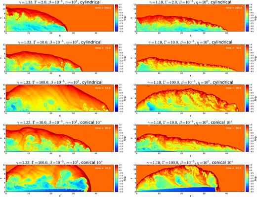
Distribution of logarithm of density for different light jet models with η = 102. Left column maps represent adiabatic (γ = 4/3) simulations and the non-adiabatic (γeff = 1.1) models are shown in the right column. Models were run with Γ = 2, Γ = 10 and Γ = 100 and the geometry was tested both for collimated (θ → 0) and wide jets. Numbers represent the time of the given snapshot in the simulation in code units.
All models evidence the formation of a bow shock structure as the jet head sweeps the ambient gas. The ambient shocked material is deposited into a cocoon that surrounds the beam. Although not obvious in the snapshots shown in Fig. 3, a double shock structure soon develops. Besides the forward bow shock, a reverse IS decelerates the jet beam and shocked jet material is also deposited into the internal part of the cocoon. The low-density portion of the cocoon is of jet shocked material, while the denser one is composed of shocked ambient gas.
The interaction of the hot shocked gas of the cocoon with the beam material drives Kelvin–Helmholtz (KH) instabilities (e.g. Birkinshaw 1996) which in turn induce both the formation of ISs pinching the beam and strong turbulent mixing and entrainment, as detected in former numerical studies of non-relativistic jets (de Gouveia Dal Pino & Benz 1993; Chernin et al. 1994).
Also, as expected from earlier studies of thermal radiative cooling jets (e.g. Blondin et al. 1990; de Gouveia Dal Pino & Benz 1993), the above effects are much stronger in the adiabatic jets (in the left panels of Fig. 3) since in these cases the internal energy of the shocked material in the cocoon is much larger than in their non-adiabatic counterparts (in the right side of Fig. 3). In the latter cases, the enthalpy of the gas in the cocoon is much smaller due to the adoption of a γ = 1.1 index to mimic thermal radiative cooling in the shocked dense ambient gas.
We should remark that in a more realistic calculation the effective value for γ would be dependent on the local properties of the plasma, and the cooling function. The adoption of a single value of γ = 1.1 for the whole system in the case of the right side models of Fig. 2 is, therefore, a simplification and the comparison with the adiabatic models should be taken with caution. These non-adiabatic models actually represent extreme examples.
Models with higher Lorentz factor obviously reach the boundary of the spatial domain earlier and therefore look less evolved. The higher propagation velocity results in a smaller loading of shocked jet material and larger spreading of the shocked ambient gas into the cocoon, which makes the driving of shear KH instabilities and turbulent entrainment less prominent than in lower Lorentz factor jets.
The models with smaller Lorentz factor (Γ = 2), specially the adiabatic one (γ = 4/3), present a cocoon with a larger portion of low-density shocked jet gas and smaller portion of high shocked ambient gas. This is because the jet beam has not enough power to drill through the dense ambient gas and also retains much more shocked jet material.
In the non-adiabatic models, the bow shock layer is thinner. The high velocity of the upstream jet flow interacting with a thin layer gives rise to the Vishniac instability (Vishniac 1994) which breaks the layer and enhances the growth of turbulence, particularly in the outer parts of the cocoon. The impact of the turbulence on the diffusion and mixing of the gas in the shocked plasma is also clear in these models.
The morphology and general properties of the density distributions, as described above, do not differ much for conical jets. This is expected since the cocoon pressure readily becomes important in the case of these low-density jets, i.e. with η < 1, resulting in similar dynamics once the jet is collimated by the cocoon.
The maximum density at the shock region is also dependent on the parameters γ and Γ. Fig. 3 indicates that larger Lorentz factors result in larger shocked densities which is consistent with the relativistic RH jump conditions (see equations 1 to 4). Also, the effective thermal radiative cooling introduced in the non-adiabatic jets by decreasing γ to 1.1 is expected, according to the jump conditions, to increase the density of the compressed shocked material at the same time that it decreases its internal pressure. The pressure reduction of the downstream gas also decreases the velocity at which it is pushed outwards. All these effects are detected in Fig. 3 and are compatible with earlier studies of non-relativistic radiative cooling jets (Blondin et al. 1990; de Gouveia Dal Pino & Benz 1993; Stone & Norman 1993). We show in Fig. 5 the Lorentz factor, density and magnetic field amplification factor at the jet axis, along y = 0, for models with η = 10−2.
4.1.2 η < 1.0 (heavy jets)
After the jet breaks the stellar envelope, it may expand over an underdense ISM. In this case, the jet density may eventually become orders of magnitude larger than that of the ambient gas. Numerical issues constrain the density contrast of the simulations, which has been fixed here to a minimum possible value η = 10−4. The larger density of the jet makes it easier to expand over the ambient medium, thus reducing and delaying certain shock effects, such as the development of a large pressure cocoon.
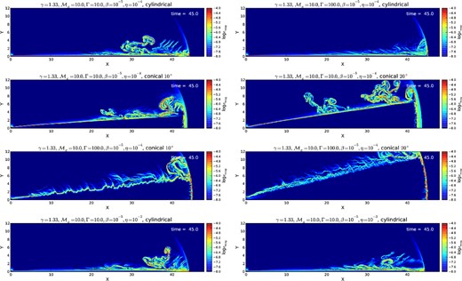
We can see in Fig. 4 that the morphology of the jet changes substantially with the increase in the jet density. For very dense jets the ambient pressure is negligible and have little impact on the propagation of the jet. The shock region shows less turbulence compared to the low-density jets.
Distribution of logarithm of density for different adiabatic, heavy jet models (with η < 1). Models were run with Γ = 10 and Γ = 100 and the geometry was tested both for collimated (θ → 0) and wide jets, with the opening angle varying between 0°, 10° and 20°. Numbers in white represent the time of the given snapshot in the simulation in code units.
Fig. 6 depicts the Lorentz factor, density and magnetic field amplification factor at the jet axis, along y = 0 for models with η = 104.
The comparison of Figs 5 and 6 (see also Figs 3 and 4) indicates that the density amplification in the interface between the cocoon and the external medium is larger with increasing density ratio η. An important fact is that for η ≫ 100 the jet is too light and has little momentum to push the ambient gas. In this case the jet decelerates quickly and does not evolve to larger radii, as already pointed out in Marti et al. (1997).
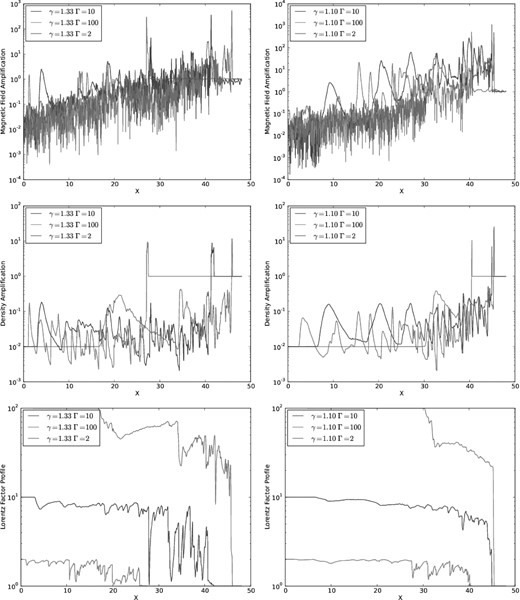
Profiles of the magnetic field amplification factor, the density amplification factor and the evolution of the Lorentz factor, obtained at y = 0, for the γ = 4/3 and 1.1 jet models, with η = 102.
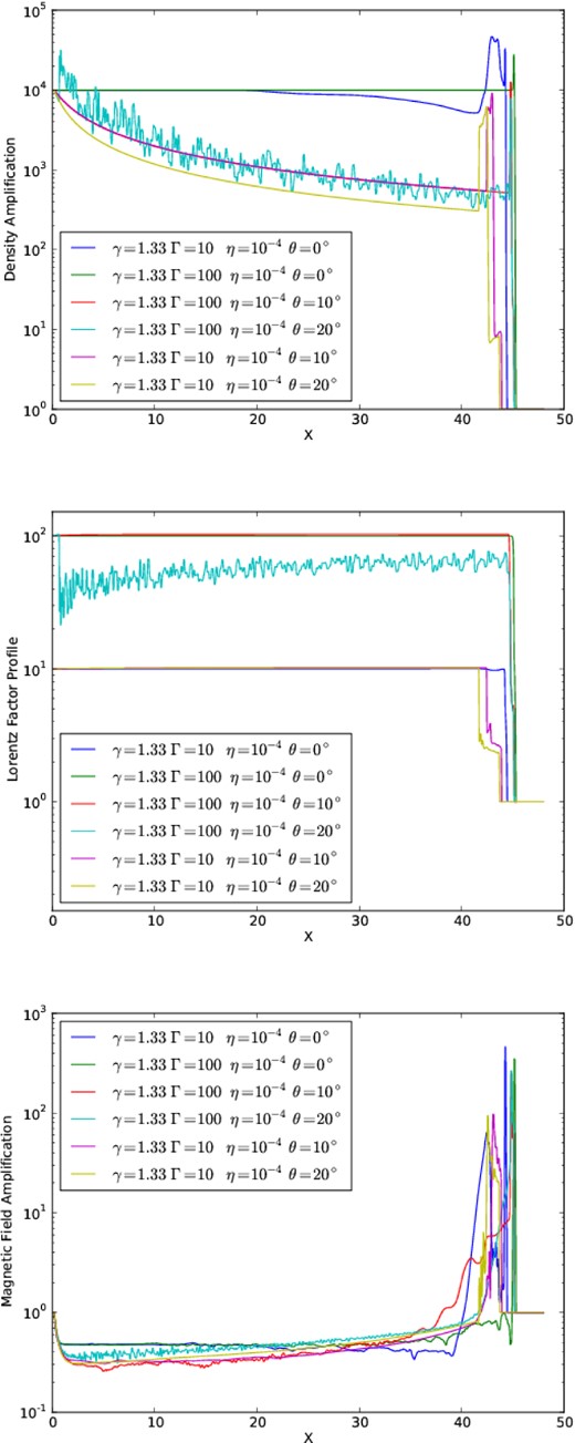
Profiles of the magnetic field amplification factor, the density amplification factor and the evolution of the Lorentz factor, obtained at y = 0, for the adiabatic (γ = 4/3) heavy jet models with η = 10−4.
In the next subsection we will see in detail how these parameters affect the spatial distribution of the magnetic field.
4.2 Magnetic energy
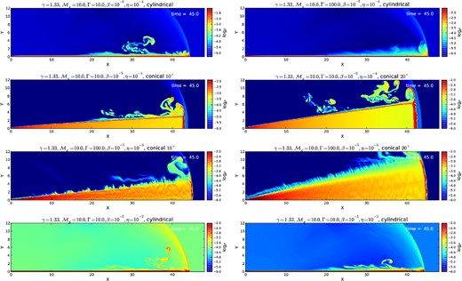
The simulated jets are initially non-magnetized, while the ambient medium is weakly magnetized, therefore the magnetization of the downstream shocked gas is mostly due to the ambient field dragged into the shock at the head and the cocoon. The spatial distribution of magnetic pressure for different models with η = 102 is shown in Fig. 7.

Same description as Fig. 3 but for the logarithm of magnetic energy density, for the jet models with η = 102.
Similarly to what is observed in the density distributions, there are striking differences in the magnetic pressure distributions of the models. For the adiabatic models (left side panels) the high-intensity magnetic fields are located at the interface (or contact discontinuity) that separates the shocked jet and ambient downstream flows (i.e. the low- and high-density portions of the cocoon). These high magnetic intensity regions basically contour the low-density region as seen in Fig. 3. The main reason for this is that the ambient magnetic field lines enter into the cocoon dragged by the shocked downstream flow. These are not able, though, to enter into the shocked jet downstream material. At the ambient downstream, the gas is deflected and flows along the contact discontinuity, as clearly seen in the adiabatic cases. The magnetic field lines, on the other hand, simply accumulate at the contact discontinuity (piling-up there). The maximum intensity of B occurs at the head of the shock for all models.
Fig. 8 shows the density distribution for the well-collimated (cylindrical) jet model AD2cyl, with γ = 4/3 and Γ = 10 at t = 90, overplotted with five selected high-intensity magnetic field lines. The streamlines depicted follow the magnetic field lines starting at the vertical coordinate y = 12.0 (top boundary) and horizontal coordinates x = [11.5, 18.0, 24.5, 31.0 and 37.5]. The ambient region presents the initial vertical field lines. At the shock regions, the lines are deflected and stretched, as expected for a super-Alfvénic flow (i.e. with velocity higher than the local Alfvén speed). As seen in Fig. 8 the field lines do not diffuse to the low-density region of the cocoon. On the contrary, they accumulate at the contact discontinuity region between the ambient shocked material and the jet shocked material, where therefore the magnetic field intensity is larger.
![Logarithmic density distribution for model AD2 of Table 1, with γ = 4/3, Γ = 10, and η = 102 at t = 90. The five lines drawn over the density plot represent magnetic field lines, each line starts at the vertical coordinate y = 12.0 (top boundary) and horizontal coordinates x = [11.5, 18.0, 24.5, 31.0 and 37.5].](https://oup.silverchair-cdn.com/oup/backfile/Content_public/Journal/mnras/446/1/10.1093/mnras/stu2104/2/m_stu2104fig8.jpeg?Expires=1750251241&Signature=pmIPJZaswoPxjsUKHuozZYfk2A0KawBpRLkiV~gzpdD~nBYwXGNd~U47lO6IFqOryRoN~ZtH4TwrEqQ2zuKoLEP8w2XNmMTnqmyAmVyL-gdttSzwFmYKuFnsew4oyRyLRW9~PE9OijDieZP86-gPfiY90V-0GAXQViFBOasSflubcFhY-UHD9Ny9oeIioJMtL2W4qdy2DvCAEbL5YUOzGTAPJnGP1M-SkBaVeDIliopbVPQvYuXSfe7MEpKMzHfYEWAI3VHeyyg8FoelQYf0~9Upye2IN1xRDTVgBqiG6042s0yExe64GlRKXw3yAQkzjGwYMXWRYPHRQRnmT-04MQ__&Key-Pair-Id=APKAIE5G5CRDK6RD3PGA)
Logarithmic density distribution for model AD2 of Table 1, with γ = 4/3, Γ = 10, and η = 102 at t = 90. The five lines drawn over the density plot represent magnetic field lines, each line starts at the vertical coordinate y = 12.0 (top boundary) and horizontal coordinates x = [11.5, 18.0, 24.5, 31.0 and 37.5].
The comparison of the adiabatic models in the left side of Fig. 7 with the non-adiabatic ones in the right hand side indicates that the maximum values of the magnetic fields are slightly larger in the non-adiabatic cases. This is compatible with the RH jump conditions for radiative cooling flows which predict a larger density of the shocked material and therefore a larger amplification of the magnetic field behind the shocks, than in the adiabatic counterparts.
Heavy jets (η < 1) on the other hand (Fig. 9) have all similar magnetic field distributions, as already noted in the case of their density distributions. The absence of a prominent cocoon reduces the internal turbulence and its role in diffusing magnetic field lines. Nevertheless, let us perform a more careful analysis of the overall results.
Same description as Fig. 3 but for the logarithm of magnetic energy density, for the jet models with η = 10−4 to η = 10−2, Γ = 10 and Γ = 100 and the opening angle varying between 0° and 20°.
The maximum magnetic energy density (|$E_{\rm max}^{\rm mag}$|) is generally located at the head of the bow shock region, as the jet expands. |$E_{\rm max}^{\rm mag}$| as a function of the location of the bow shock head in the x-direction is shown in Fig. 10. Each snapshot created from the simulations is shown as a point in the plot. The top and middle diagrams show the results for all collimated jets (with light jets being depicted in the top panel and heavy jets in the middle panel). The solid line represents the correlation |$E_{\rm mag}^{\rm max} \propto x^2$|, for comparison. Notice that the line is not a statistical fit, but is in good agreement with all models with θ = 0. Most strikingly, all models, independent on the Lorenz factor, the polytropic index, or the density ratio η, present similar |$E_{\rm mag}^{\rm max}$| at the same position of the shock head. This result is consistent with the magnetic field pile-up effect discussed in Section 2 and with equation (7) which predicts Bampl ∝ xα, with a maximum α ≃ 1 for a compressed magnetic field parallel to the discontinuity.
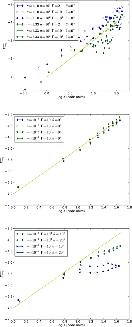
Maximum magnetic energy density (in erg cm−3) as a function of the jet head position; top: cylindrical (θ = 0) light jets, middle: cylindrical (θ = 0) heavy jets, and bottom: wide jets, with different Lorentz factors, and opening angles. The correlation |$E_{\rm max}^{\rm mag} \propto B_{\rm max}^2 \propto x^2$| is very similar for all collimated jet models. The solid line with a slope of ζ = 2 was drawn for reference.
In the bottom diagram of Fig. 10, we show the evolution of the maximum magnetic field intensity for the conical jets. The dependence of |$E_{\rm max}^{\rm mag}$| with the opening angle θ and Γ in consistence with the analytical prediction of equation (11) is clear.
The results above clearly show that the pile-up effect is maximized in the case of θ → 0, as one should expect. In fact, the piling-up is maximized in the forward shock region where the jet velocity is nearly normal to the magnetic field lines. Thus, although a conical geometry may offer a larger area for the forward shock to sweep the ambient magnetic lines, most of the shock front is oblique which will weaken the piling-up. Also, the net flux of plasma out of the shock region is limited (causality is not broken here), and once the Mach disc becomes large enough local enthalpy cannot be considered as constant any longer. After this transition phase the shock width scales linearly with x and the pile-up effect ceases. This is well accounted in equation (11).
We stress here that the results obtained in Fig. 10 are nearly insensitive to the jet-ambient density ratio η. This result is actually not surprising. The accumulation of the compressed ambient magnetic field lines depends on η through the propagation velocity of the forward bow shock into the ambient medium (see equations 7 to 9), i.e., βbs = βj(1 + L−1/2), where L measures the ratio between the jet energy density and the ambient rest mass energy density, |$L= \mu _{\rm j} \Gamma _{\rm j}^2/ \eta$|, and μj ∼ 1 is the specific enthalpy of the jet (Bromberg et al. 2011). For the typical large values of Γj ∼ 10–100 of GRB jets, it turns out that in general L ≪ 1, even for η varying in a broad range like the one investigated here η = 10−4 to 102, so that βbs and the pile-up effect are nearly insensitive to this parameter.
4.3 Structure function of |${\boldsymbol B}$| and its correlation length
The amplification of B as seen in these models is particularly important because, regardless of the magnetization of the jet itself, as the beam sweeps the ambient gas, the ambient magnetic field lines are dragged, amplified by compression, and piled-up into the shock region. Also, as important as the total magnetic field intensity is its correlation length.
In any model of magnetic field amplification, theoretical predictions must also provide arguments for obtaining sustainable large-scale magnetic fields.
We performed the SF calculations for the magnetic field lines anchored into the shock head only – this because we focus on determining the correlation length of the maximum amplified magnetic fields. In Fig. 11 we present the SFs (S) obtained for the selected adiabatic models. The non-adiabatic models were not plotted to avoid superposition with the depicted curves, as they present very similar profiles to those of the adiabatic counterparts.
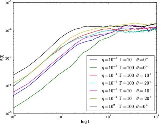
SFs of magnetic field lines for models varying the parameters η, Γ, and the opening angle. The horizontal axis is shown in number of pixels. Notice that the SFs are calculated along the magnetic field lines and the total pathways are therefore larger than the size of the box.
For light jets with η = 102, the saturation of the SFs occurs, in all models, at length scales which represent lsat ≃ 0.35–0.46 in code units. These values correspond to approximately three to five times the shock thickness λ for the adiabatic and non-adiabatic models, respectively. Heavy jets with η = 10−4 present larger coherence lengths. For these models the saturation of the SFs occurs at length scales in the range of lsat ≃ 60–200 pixels, depending on the opening angle of the jet, which represents lsat ≃ 2.3 in code units. Larger coherence lengths occur for smaller opening angles.
5 DISCUSSION AND CONCLUSIONS
In this work, we have explored the possible magnetic field amplification and correlation lengths behind the shock head region of non-magnetized, light and heavy relativistic jets propagating into weakly magnetized environments aiming at comparisons with GRB jet afterglows scenarios in a matter-dominated regime. For this we have carried out 2D RMHD simulations considering different values of the jet bulk Lorentz factor (Γ = 2, 10, and 100) and the density ratio between the jet and the environment (η = ρamb/ρj = 10−4–102). We have focused on relativistic adiabatic jets (with an adiabatic index γ = 4/3), but for comparison have also considered systems with γ = 1.1 in order to mimic the effects of a potential strong thermal radiative cooling in the shocked ambient material at the jet head. All the jets were expanded for approximately the same extension, so that the jet with the highest Lorentz factor was the less evolved one. We have also tested the effects of the jet geometry, considering different opening angles from θ = 0° (cylindrical jet) to θ = 20°. Our findings are summarized below.
The magnetic field is amplified by shock compression and accumulates at the contact discontinuity (pile-up effect), with a maximum value that increases with the distance as the jet propagates. The predicted relationship between the magnetic field intensity and the distance as described in equations (7), (8) and (11), was confirmed by the simulations. In particular, we have found that the increase in the magnetic field amplification, though initially similar for both collimated and wide jets, saturates earlier for increasing jet opening angles. This effect is smaller as the jet Lorentz factor increases. These results have been found to be nearly insensitive to the density ratio η, but heavier jets present larger magnetic field coherence lengths than lighter ones. Also smaller coherence lengths have been found for larger jet opening angles. In summary, heavy, collimated jets tend to maximize the piling-up and the coherence length of the magnetic field lines.
The above results have been also found to be nearly independent of the adiabatic index (γ), although the maximum intensities of the compressed magnetic fields are a little larger in the non-adiabatic cases, as one should expect from the jump conditions and the larger density amplification behind the shocks in these cases. This general behaviour can be explained by the fact that, after a maximum compression behind the double shock structure at the jet head, the magnetized shocked material is forced to expand sideways, along the cocoon that surrounds the jet. Apparently, all the cases reach similar saturation ratios for the density and magnetic field at the contact discontinuity, regardless of the differences in the jet upstream conditions. Nevertheless, these differences obviously affect the final state of the shocked material that deposits into the cocoon which is clearly distinct in each of the simulated systems as discussed in Section 4.1 (see Figs 3 and 7).
We notice here that in more realistic calculations, with a more consistent treatment of the radiative cooling, the effective value of γ would not be homogeneous over the whole computational domain. The ‘non-adiabatic’ models above actually represent extreme examples. In more realistic models, with an adiabatic jet beam (with γ = 4/3) interacting with a radiative cooling cocoon, we would expect the beam structure to be less affected by the shocked cooled gas of the cocoon than in Fig. 3 and the propagation velocity of the jet head slightly smaller.
Since we have considered a very broad parametric space, the above results can be in principle applicable to all classes of relativistic jets, including microquasars, AGNs and GRBs, but below we will discuss the implications for the afterglow emission of GRB jets.
5.1 Implications for GRB afterglows
5.1.1 Magnetic field amplification
Observations of the afterglow phase of GRBs are explained by synchrotron emission of electrons interacting with nearly equipartition magnetic field intensities of Bequip ∼ 1 G, at distances of ∼1015 cm away from the central source (see review of Piran 2005). As explained in Section 2 the equipartition radius for the magnetic field amplification depends on the shock width λ, which can be roughly estimated from equation (10) (see also equation 11). In this equation, as stressed in Section 2, we need the jet radius at the breakout from the stellar progenitor envelope. This can be estimated from previous analytical and numerical studies of GRB jets (e.g. Zhang et al. 2003; Mizuta & Aloy 2009; Levinson & Begelman 2013; Mizuta & Ioka 2013; Bromberg et al. 2014). For a Poynting flux-dominated jet propagating inside the envelope of a Wolf–Rayet progenitor, analytical predictions suggest that rj ∼ rL ∼ 107 cm, where rL is the radius of the light cylinder near the source (Levinson & Begelman 2013; Bromberg et al. 2014), while for matter-dominated jets rj can be larger. Numerical simulations indicate rj ∼ 109 cm (Zhang et al. 2003; Mizuta & Aloy 2009; Mizuta & Ioka 2013). Thus, if we assume rj at the breakout to be rj ∼ 107–109 cm, and η = 10−4–102, then we obtain λ ∼ 103–1011 cm. Despite the simplified geometry, and absence of magnetic field, assumed on the estimation of equation (10), these values are in rough agreement with the λ/rj ratio observed in the simulations. In this case, equipartition should occur at xbs ∼ 109–1017 cm. These values are compatible with the observed afterglow distances (∼1015 cm).
For jets with opening angles, i.e. θj > 0°, the maximum amplification is reduced. Our results indicate that wide jets present similar behaviour as their cylindrical collimated counterparts at small distances, for which the conclusions made above would be sustained. This is not true though at larger distances. While the well-collimated jets result in a quasi-indefinitely increase of magnetic pressure (until equipartition is reached), jets with large opening angles saturate at earlier stages. Here the main cause for the saturation is not equipartition but the widening of the shock region width. In conical jets the ratio between the fluxes out and inwards the shocked region becomes smaller with time, resulting in the width growth. Models with θ = 20° saturate with Bmax approximately 1 order of magnitude smaller than those with θ = 10°. As the width of the shock region increases, the amplification of the magnetic field is smaller for a lower saturation value in agreement with equation (7). For instance, for a tan θ ∼ 0.1 and Γ ∼ 102 jet, the saturation radius is expected to be at ≃103rj ∼ 1012 cm and, as shown above, this length scale would be large enough to amplify the magnetic fields to the observed intensities.
However, despite the apparent sufficient amplification factors obtained from the pile-up process, the large magnetization of the observed afterglow emission cannot be fully explained yet. In the current GRB paradigm, adopted in this work, the afterglow emission is assumed to be radiated from the freshly injected plasma at vicinity of the shock. It should be further noticed that the freshly injected plasma, just downstream of the shock, is weakly magnetized.4 The main effect of pile-up only occurs as the matter flows further downstream whereas the frozen field slowly grows. Though the field strength could be large it peaks at the contact discontinuity region, which is at a distance ∼λ of the freshly injected shocked plasma, where particles are supposed to accelerate. Therefore, the pile-up effect, even if it is strong enough, may not directly affect the afterglow emission in such a scenario, and would not provide ‘the’ solution to the magnetization problem in GRBs.
5.1.2 Correlation lengths
Also, by means of second-order SFs, we obtained the correlation lengths of the amplified magnetic fields at the jet head. We find lcorr ∼ 3–5λ ∼ 108–1012 cm for light jets, and ∼109–1014 cm for the heavy jet models. There is no obvious trend between the correlation length and the jet opening angle. For the Weibel instability the correlation lengths obtained are of the order of the plasma skin depth, i.e. δ = (c/ωp) ∼ 106 cm, while observations point towards much larger correlation lengths, of 1016 cm (e.g. Waxman 2006).
Still the values obtained in this work are 2 orders of magnitude smaller than those obtained from observations. Since our models revealed that the correlation length depends on the jet-to-ambient gas density ratio, heavier jets, compared to those simulated here, would result in larger lcorr, closer to observations. Another possible solution to this problem is that, due to the strong downstream turbulence as seen in part of our models, magnetic reconnection could be induced resulting in more uniform fields. Considering that the equipartition occurs at short time-scales (specially for jets), any magnetic energy loss due to reconnection would be shortly replenished by further piled-up field lines. It is possible then that the field lines would have larger observed correlation lengths once the systems reach the afterglow phase.
Our results show that the correlation lengths in the shock fronts are still around 2 orders of magnitude smaller than those inferred from GRB observations. Therefore other possibilities, such as the magnetization of the jet must be explored in future works. The recent polarization observations by Wiersema et al. (2014) indicate that this may be the correct way to solve this question.
5.2 Final remarks
Two further important remarks are in order. First, we have assumed a 2D jet geometry. A more realistic 3D geometry can reduce the pile-up efficiency since this geometry allows another degree of freedom for the magnetic field lines (and gas) to leave the shock region. However, since in this case the degree of freedom of field lines is still smaller than that of the gas, the pile-up must still occur, though not as efficient as in the two-dimensional well-collimated jet case. We stress that the main goal of this work was not to reproduce the actual emission properties of the afterglow, but to verify if the magnetic field could be amplified in the jet-envelope shock context. In order to determine exactly the emission properties, on top of the amplification process, three-dimensional simulations are mandatory.
A third dimension will naturally introduce another degree of freedom for the downstream flow, which implies an extra dimension to which magnetic field lines may be carried away from the shock region thus decreasing the pile-up effect. We may therefore expect that in a 3D jet model the amplification of the magnetic field intensity will slow down, but the final picture of the pile-up in this case is still unknown. Another possible effect that was not taken into account in our study regards the fact that, at the time that the jet breaks out from the stellar surface into the ambient medium, the GRB central engine has probably turned off already. This implies that the continuous injection should stop, giving place to a propagating jet parcel with a forward bow shock at the head slowly detaching from the reverse shock. This effect will also weaken the piling-up of the magnetic field in the bow shock. Both effects will be investigated in depth in a forthcoming work.
However, even in the case of efficient pile-up we must be careful in attributing to this mechanism the solution for the magnetization problem in the afterglow emission. The magnetic energy in our models has been found to be concentrated at the contact discontinuity while the emitting particles are expected to be located at the downstream side of the shock surface. A large distance between these two different regions result in an effective low magnetization where the emitting particles actually are. This issue must be pursued in forthcoming works.
Finally, as stressed before, the afterglow emission is generally believed to be due to relativistic particles accelerated by a first-order Fermi process occurring mostly at the shock region, at the jet head. Examining Fig. 7, we note that other regions in the beam and the cocoon than the shock head itself have also reached a magnetized turbulent structure with high-intensity magnetic fields. These magnetic fields, in part also amplified by the instabilities developed in the cocoon and by turbulent shear, can equally help to accelerate particles to relativistic velocities. In these regions, first-order Fermi acceleration by magnetic reconnection, as first proposed by de Gouveia dal Pino & Lazarian (2005), can be also very efficient, as well as second-order Fermi to pre-accelerate the particles, as indicated by recent numerical MHD studies of particle acceleration in different domains of magnetic reconnection (Kowal et al. 2012) (see also de Gouveia Dal Pino & Kowal 2013, for a review). This issue will be further explored by means of 'in situ' particle acceleration simulations in relativistic jets as in de Gouveia Dal Pino & Kowal (2013) where preliminary tests have been presented (see also applications to GRBs in Giannios 2010 and Cerutti et al. 2013).
GRS thanks CNPQ for financial support. DFG thanks the European Research Council (ADG-2011 ECOGAL) and the Brazilian agencies CNPq (No. 300382/2008-1), CAPES (3400-13-1) and FAPESP (No. 2011/12909-8) for financial support. GK thanks FAPESP (No. 2009/50053-8, 2011/51275-4, 2013/04073-2, 2013/18815-0) for financial support. EMGDP thanks FAPESP (No. 2006/50654-3) and CNPq (306598/2009-4) for financial support. The authors also acknowledge very fruitful discussions with T. Piran, J. Stone and G. Lugones. This work has made use of the computing facilities of the Laboratory of Astroinformatics (IAG/USP, NAT/Unicsul), purchased by FAPESP (grant 2009/54006-4), and of the Hydra cluster at EACH-USP.
Which is obtained from momentum flux conservation assuming that the ambient pressure is negligible, as the gas is cold, and the jet pressure is much smaller than the jet shock ram pressure.
The 2D approach in this work means that the system is considered in a planar symmetry, not axial, since the external magnetic field has to be kept uniform. Such approach is limited, obviously, and underestimates the dynamics of the flows perpendicular to the plane, i.e. orthogonal to the magnetic field. A more detailed discussion about this is presented later in the article, but a more comprehensive picture will be provided in a future work where a full 3D modelling is presented.
Long before Taub (1948) had shown that in order to preserve the consistency with the relativistic kinetic theory, the specific enthalpy μ has to satisfy the inequality: (μ − Θ)(μ − 4Θ) ≥ 1, where Θ = p/ρ and μ is the enthalpy of the relativistic gas and their proposed equation of state satisfies the Taub inequality.
As given by the standard RH conditions.
