


Abstract
Spectroscopic and photometric observations of the nearby Type Ia Supernova (SN Ia) SN 2014J are presented. Spectroscopic observations were taken −8 to +10 d relative to B-band maximum, using FRODOSpec, a multipurpose integral-field unit spectrograph. The observations range from 3900 to 9000 Å. SN 2014J is located in M82 which makes it the closest SN Ia studied in at least the last 28 yr. It is a spectroscopically normal SN Ia with high-velocity features. We model the spectra of SN 2014J with a Monte Carlo radiative transfer code, using the abundance tomography technique. SN 2014J is highly reddened, with a host galaxy extinction of E(B − V) = 1.2 (RV = 1.38). It has a Δm15(B) of 1.08 ± 0.03 when corrected for extinction. As SN 2014J is a normal SN Ia, the density structure of the classical W7 model was selected. The model and photometric luminosities are both consistent with B-band maximum occurring on JD 245 6690.4 ± 0.12. The abundance of the SN 2014J behaves like other normal SN Ia, with significant amounts of silicon (12 per cent by mass) and sulphur (9 per cent by mass) at high velocities (12 300 km s−1) and the low-velocity ejecta (v < 6500 km s−1) consists almost entirely of 56Ni.
1 INTRODUCTION
Supernovae are important and much-studied astrophysical events. For example, they are the main producers of heavy elements in the Universe, and Type Ia supernovae (SNe Ia) produce most of the iron-group materials (Iwamoto 1999). SNe Ia have also been confirmed as the best cosmological ‘standard candles’ and as a result there has been a dramatic increase in the rate at which they are observed. They were integral in the discovery of the acceleration of the universe (Riess 1998; Perlmutter et al. 1999), and are now an important cosmological probe in improving the understanding of the nature of the positive cosmological constant. However, the true intrinsic properties of SN Ia are not yet fully understood, including their progenitor system and diversity in luminosity (e.g. SN 1991bg; Leibundgut et al. 1993). There are currently two favoured progenitor scenarios. The first is a carbon/oxygen White Dwarf (WD) which accretes mass from a non-electron-degenerate companion star (Nomoto, Iwamoto & Kishimoto 1997). In this single degenerate (SD) scenario (Hoyle & Fowler 1960), the WD can explode when it approaches the Chandrasekhar mass. There are several suggested ways in which this can occur, including a subsonic explosion (a deflagration) and a supersonic explosion (a detonation) as well as an explosion with a transition to a detonation. In the fully subsonic explosion there is not enough energy to fully power the SN Ia and in supersonic explosion there is too much 56Ni in the ejecta. Therefore, the transition may be the correct explosion model for SN Ia (Khokhlov 1991). Two further SD explosion models are fast deflagration and sub-Chandrasekhar-mass explosions (Nomoto, Thielemann & Yokoi 1984; Livne & Arnett 1995). The other suggested progenitor model is a double degenerate (DD) scenario, where the SN results from the merger of two WDs (Iben & Tutukov 1984).
Thanks to the dramatic increase in observations of SN Ia, in the last two decades, it is now possible to obtain good spectral time series of them. These time series can span from before B-band maximum to the nebular phase. One approach to fully understand the composition and progenitor system of an individual SN Ia, is to use Monte Carlo (MC) radiative transfer code and the abundance tomography technique (Mazzali 2000; Stehle et al. 2005). This approach models early-time observed spectra, by changing input parameters such as the chemical abundance, bolometric luminosity, photospheric velocity and time since explosion. The abundance tomography approach exploits the fact that with time deeper and deeper layers of the ejecta become visible. By modelling time series, spectral information about the abundances at different depths can be extracted, with this it is possible to reconstruct the abundance stratification from the observational data. This approach directly links the theoretical models and observed spectra to help one get a true understanding of the early-time evolution of a SN Ia. The MC radiative transfer code has been successfully used in modelling many SNe Ia including 2003du (Tanaka et al. 2011), 2004eo (Mazzali et al. 2008) and 2011fe (Mazzali, Sullivan & Hachinger 2014).
We present photometric and spectroscopic data taken with the Liverpool Telescope (LT) and Isaac Newton Telescope (INT) for SN 2014J, and then apply the aforementioned modelling techniques with the aim of inferring the ejecta properties on the SN. SN 2014J is a spectroscopically normal SN Ia, which has high-velocity features. It is of particular interest as it is the closest SN Ia in at least the last 28 yr, and possibly the closest in the last 410 yr (Foley et al. 2014). As technology has dramatically improved in this time, this SN gives us a unique opportunity to intensely observe, analyse and model a SN Ia with modern technology. SN 2014J is located at RA = 9:55:42 Dec. = 69:40:26.0 (J2000), and is in M82 which is at a distance of 3.77 ± 0.66 Mpc. This value was obtained from the mean distance from NED,1 which used two methods PNLF (Planetary Nebula Luminosity Function) and TRGB (Tip of the Red Giant Branch) to derive it. However, it should be noted that Foley et al. (2014) derive a distance of 3.3 Mpc. M82 is known for having a large amount of star formation; hence, it has a large amount of dust (Hutton et al. 2014). Because of this, SN 2014J is highly and unusually reddened. It does not follow the average galactic reddening law of RV = 3.1. Detailed investigations into the host galaxy extinction were produced by Amanullah et al. (2014) and Foley et al. (2014). With our modelling approach, we optimize the published extinction values which produce the best fits of SN 2014J from the spectra.
The paper starts with a report of the observations (Section 2), which includes 12 spectra taken from −8 to +10 d. In the following section (Section 3), we discuss the aperture photometry, including the SDSS g′r′i′ light curves. In Section 4, we present the fully reduced and calibrated spectra. The next section (Section 5) discusses the MC radiative transfer technique. In Section 6, the modelled spectra of 10 early-time epochs are presented and discussed. Afterwards (Section 7), we discuss the abundance stratification we have inferred. Finally, the results are summarized and conclusions are drawn from them (Section 8).
2 OBSERVATIONS
SN 2014J was discovered on 2014/01/21.810 by S. J. Fossey at the UCL observatory (Fossey et al. 2014). The LT carried out detailed spectroscopic and photometric observations, starting from 2014 January 22. The LT is a 2.0 metre fully robotic telescope located at Observatorio del Roque de los Muchachos (ORM) on La Palma. Photometric observations were obtained using IO:O, an optical imaging camera which has a field of view (FOV) of 10 arcmin2. The photometric images were acquired in three pass-bands (SDSS g′r′i′). Spectra were obtained using FRODOSpec, a multipurpose integral-field unit spectrograph, at 10 epochs from −8 to +10 d relative to B-band maximum. FRODOSpec consists of blue and red arms which cover 3900–5700 Å and 5800–9400 Å, respectively.
The IO:O pipeline carries out basic reduction of photometric data; this consists of bias subtraction, trimming of the overscan regions and flat fielding. FRODOSpec has two independent reduction pipelines. The first one, L1, performs bias subtraction, overscan trimming and CCD flat fielding, whereas the second one, L2, is specific to FRODOSpec (Barnsley, Smith & Steele 2012). It produces sky-subtracted row-stacked spectra, which were used in this paper. No host galaxy subtraction has been performed when analysing the spectra, as no images were available. However, the sky subtraction routine in the FRODOSpec pipeline removes most of the flux from the M82, meaning that any flux which has not been subtracted should be negligible.
We also have two spectra obtained using the 2.5 m INT, located at ORM on La Palma. The Intermediate Dispersion Spectrograph (IDS), a long-slit spectrograph on the INT, was used with the R1200Y grating and RED+2 camera. The INT observations were made with the slit at the parallactic angle. Table 1 is a log of spectroscopic observations of SN 2014J.
Log of spectroscopic observations of SN 2014J.
| Epoch | MJDa | Phaseb | Exp. time | Instrument |
|---|---|---|---|---|
| (d) | (s) | |||
| 2014-01-26 | 56684.12 | −8 | 500 | FRODOSpec |
| 2014-01-27 | 56685.12 | −7 | 500 | FRODOSpec |
| 2014-02-03 | 56692.01 | +0 | 600 | FRODOSpec |
| 2014-02-04 | 56692.90 | +1 | 600 | FRODOSpec |
| 2014-02-04 | 56693.13 | +1 | 3 × 120 | INT |
| 2014-02-05 | 56693.89 | +2 | 600 | FRODOSpec |
| 2014-02-06 | 56694.96 | +3 | 600 | FRODOSpec |
| 2014-02-07 | 56695.89 | +4 | 500 | FRODOSpec |
| 2014-02-07 | 56696.13 | +4 | 3 × 120 | INT |
| 2014-02-08 | 56696.92 | +5 | 500 | FROSOSpec |
| 2014-02-09 | 56697.97 | +6 | 500 | FRODOSpec |
| 2014-02-11 | 56699.88 | +8 | 500 | FRODOSpec |
| 2014-02-13 | 56701.877 | +10 | 500 | FRODOSpec |
Notes:aObservation in MJD date.
bRelative to B-band maximum.
3 PHOTOMETRY
Photometric reduction was carried out using the iraf2 package daophot. Instrumental magnitudes of the SN and stars within the field were obtained. In order to produce the calibrated magnitudes of the SN, the colour terms and zero-points were required. For the g′r′ and i′ filters, the colour terms were obtained by using the standard star images, taken on the same night as the observations, and comparing their instrumental magnitudes to the APASS catalogue magnitudes (Henden et al. 2009). IO:O typically requires an exposure time of over 10 s for good photometry, due to the amount of time it takes for the shutter to open and close. We typically have an exposure time of 2 s in our photometric images. Therefore, stars at the edge of the FOV will be exposed for a shorter period of time than ones in the centre of the field. To overcome this, the zero-points were calculated using a single star, RA = 9:55:35 Dec = 69:38:55 (J2000), close to SN 2014J. The main source of error in the photometry was calculating the zero-points; if the calibration star was saturated the magnitude was ignored. As we do not have pre-explosion images of M82 using the LT, we have not subtracted the host galaxy from the photometry. To calculate how much this host galaxy flux affects our photometry, we used SDSS images of M82. We carried out aperture photometry, using the same aperture size as the LT images, on the location of the SN pre-explosion and a standard star in the FOV. From this, we found that the highest value the photometry can deviate by, owing to the missing host galaxy subtraction, is 2.35 per cent mag in the i′ band, 1 per cent mag in the r′ band and 0.5 per cent mag in the g′ band.
SN 2014J was observed at a daily cadence from MJD 56680.20 to 56743.84. g′r′i′ light curves were produced (Fig. 1). There was a gap in observations between 2014 February 13 and February 21, due to poor weather conditions on La Palma. g′-band maximum occurred on February 03, which is consistent with the maximum in the B pass-bands (Tsvetkov et al. 2014). We found that g′-band maximum was 11.42 ± 0.09 mag, r′-band maximum was 10.16 ± 0.03 mag and i′-band maximum was 10.20 ± 0.05 mag. The distance modulus we use for M82 was taken from NED, μ = 27.86 mag. Therefore, at maximum, SN 2014J had an absolute g′-band magnitude of −16.44 mag, an r′-band magnitude of −17.68 mag and an i′-band magnitude of −17.66 mag, before correction for extinction.
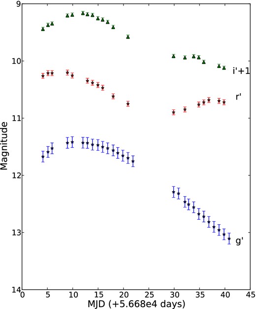
Aperture photometry light curves, produced using LT data. SDSS g′r′i′ light curves are presented. The errors on the photometry appear to be constant; this is due to the catalogue error on the zero-point star dominating.
The foreground Galactic extinction of SN 2014J is E(B − V) = 0.05 mag (RV = 3.1; Amanullah et al. 2014; Foley et al. 2014). A large host galaxy reddening of SN 2014J was inferred by Amanullah et al. (2014) and Foley et al. (2014). The values obtained for the colour excess using the CCM law (Cardelli, Clayton & Mathis 1989) by Foley et al. (2014) were E(B − V) = 1.24 ± 0.1 mag and RV = 1.44 ± 0.06. However, Foley et al. (2014) state that the best solution to the extinction of SN 2014J is using a two-component circumstellar scattering and dust reddening model. Amanullah et al. (2014) use photometric comparisons to SN 2011fe to obtain the best-fit for the reddening values. Using the FTZ reddening law (Fitzpatrick 1999) between −5 and +35 d relative to B-band maximum it was found that E(B − V) = 1.29 ± 0.02 mag and an RV of 1.3 ± 0.1 with a χ2/dof = 3.3. It should be noted that the RV value is much lower than the typical Galactic average of RV = 3.1. We use a host galaxy extinction of E(B − V) = 1.2 with RV = 1.38; details of why we use these values can be found in Section 6. The attenuation of the flux in B and V is similar with the values of Amanullah et al. (2014) and Foley et al. (2014).
Foley et al. (2014) and Marion et al. (2014) have published photometric and spectroscopic observations of SN 2014J. They report Δm15(B) to be 1.01–1.08 mag when corrected for host galaxy extinction, and 1.11 ± 0.02 mag when not corrected for host galaxy extinction, respectively. We analysed the LT SDSS g′- and r′-band photometry with the sifto (Conley et al. 2008) light-curve fitter to obtain the stretch, V-band maximum and tBmax (see Fig. 2). Using the g′ and r′ bands, we obtained a stretch of 1.083 ± 0.06, which corresponds to a Δm15(B) = 0.88 ± 0.08 using the relation from Conley et al. (2008). However, using only the r′-band light curve produces a stretch of 1.035 ± 0.08 and therefore a Δm15(B) of 0.95 ± 0.12. When corrected for host galaxy extinction, E(B − V) = 1.2 (RV = 1.38), using the relation from Phillips et al. (1999), the B-band decline rate is found to be 1.00 ± 0.06 or 1.07 ± 0.08 for g′ and r′ bands and r′ band, respectively. These decline rates are consistent with those of Foley et al. (2014). However, the correction of Phillips et al. (1999) for obtaining ‘reddening-free’ Δm15 values from the observed values was derived assuming an RV = 3.1. To check the sensitivity of this correction to RV, we carried out our own calculation of the effect of dust reddening on Δm15(B) for RV = 3.1 and V1.4 using the published optical spectrophotometry of SN 2011fe (Pereira et al. 2013) and the Hsiao SN Ia spectral template (Hsiao et al. 2007). The spectra were reddened for values of E(B − V) = 0.0–2.0 using the iraf DEREDDEN task, which implements the CCM law. Synthetic magnitudes were calculated using the Bessell (1990) B pass-band, and the B-band decline rate was measured for each value of E(B − V). Fig. 3 shows the results, including a comparison with the approximate relation given by Phillips et al. (1999). As is seen, the effect on Δm15(B) of changing the value of RV from 3.1 to 1.4 is small. For E(B − V) = 1.2 and RV = 1.38 application of these calculations to our sifto-measured decline rates gives Δm15(B) = 0.98 ± 0.08 or 1.05 ± 0.12, for the g′ and r′ bands and r′ band, respectively, using the 2011fe spectra, and Δm15(B) = 0.95 ± 0.08 or 1.02 ± 0.12 using the Hsiao template. The value of the decline rate may increase when the full host galaxy subtraction can be carried out on the photometry. Foley et al. (2014) state that the V-band maximum was 10.61 ± 0.05, whereas our fitting obtains this to be 10.66 ± 0.02. We obtain a tBmax which is consistent with the values found by Foley et al. (2014).
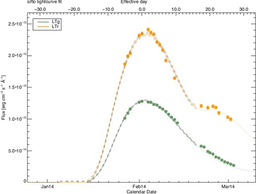
sifto SN 2014J light-curve fits.
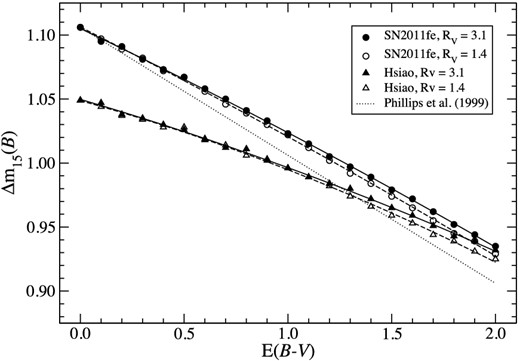
Dependence of Δm15(B) on E(B − V) for different values of RV, using SN 2011fe spectrophotometry and the Hsiao template.
4 SPECTROSCOPY
The LT data spectroscopic reduction was done in two halves, corresponding to the blue and red arms of FRODOSpec. Each spectrum was manually searched through to select fibres which had signal. An appropriate top threshold was applied, to ensure cosmic rays were not affecting the spectrum. The signals from these fibres were combined; the spectra were formed using the onedspeciraf package. The SN spectra were calibrated in flux using spectra of Feige34. The accuracy of the flux calibration process was confirmed by a successful calibration of the star back on to itself. This was done by running the calibration process on the observations of the standard star, and checking this against the iraf data for the star. The INT data were reduced using the starlink software (Disney & Wallace 1982). The spectrophotometric standard used to reduce the INT data was Feige66.
A full plot of a SN 2014J spectrum with the main absorption lines labelled is found in Fig. 4 and the early-time spectral evolution of SN 2014J is plotted in Fig. 5. The spectra have a very strong Si ii 6355 Å absorption line. They also have high-velocity features at early epochs; the main high-velocity feature is exhibited by the Ca ii IR triplet around ∼7900 Å. Furthermore, at even earlier times up to −12 d Goobar et al. (2014) have found a strong high-velocity feature of Si ii 6355 Å. Fig. 5 demonstrates the extent of the reddening, which means that the flux in the blue arm is extremely suppressed. The evolution of the Si ii 6355 Å line can be seen in Table 2. As expected, as the photosphere recedes, the velocity of the ejecta decreases and hence the wavelength of the absorption line increases, although this may not always be apparent over smaller intervals. This is due to the resolution of the spectra and the errors on the velocity. The velocity gradient from the Si ii 6355 Å line between +0 and +9 d relative to B-band maximum is 58.8 km s−1 day−1. This makes SN 2014J a low-velocity gradient SN Ia (Benetti et al. 2005). It can be seen in the LT post-maximum spectra at +6, +8 and +10 d that P-Cygni re-emission redwards of the Si ii 6355 Å absorption has a flat top, which is also visible in the HST data at +11.3 d (Foley et al. 2014). A full plot of a SN 2014J spectrum with the main absorption lines labelled is found in Fig. 4.
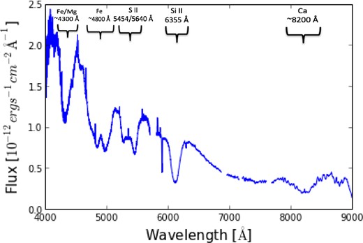
An overview of the features of SN 2014J. This spectrum has been dereddened and was taken at B-band maximum.
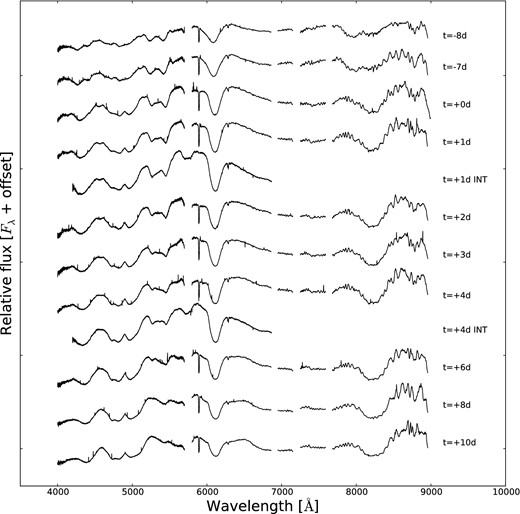
All spectral observations of SN 2014J, LT and INT. The time is given relative to rest-frame B-band maximum. The spectra have not been corrected for reddening. There were no data collected between 5700–5800 Å for the LT observations and the two atmospheric absorption lines have been removed. All of the plots have been offset by an arbitrary amount for the purpose of presentation.
Log of the Si ii 6355 Å absorption line velocities.
| Epoch | MJDa | Phaseb | Velocityc |
|---|---|---|---|
| (d) | (d) | (km s−1) | |
| 2014-01-26 | 56684.12 | −8 | 12 973 |
| 2014-01-27 | 56685.12 | −7 | 12 643 |
| 2014-02-03 | 56692.01 | +0 | 11 758 |
| 2014-02-04 | 56692.9 | +1 | 11 697 |
| 2014-02-05 | 56693.89 | +2 | 11 686 |
| 2014-02-06 | 56694.96 | +3 | 11 552 |
| 2014-02-07 | 56695.89 | +4 | 11 640 |
| 2014-02-08 | 56696.89 | +5 | 11 412 |
| 2014-02-09 | 56697.97 | +6 | 11 529 |
| 2014-02-11 | 56709.87 | +8 | 11 408 |
| 2014-02-13 | 56701.877 | +10 | 11 228 |
Notes:aModified Julian Day number.
bRelative to B-band maximum (days).
cVelocity of the Si ii 6355 Å absorption line.
By using the correlation between the ratio of the depth of the silicon lines, 5972 and 6355 Å, and absolute magnitude and therefore Δm15(B) (Nugent et al. 1995) we have obtained a photometry-independent approximation for the Δm15(B) of SN 2014J. We used the INT spectra from +1 d to do this, as the INT data cover the 5972 Å feature. We derive Δm15(B) = 1.11 ± 0.02, which is consistent with the values found by Marion et al. (2014) and Foley et al. (2014). Furthermore, it is possible to use the Equivalent Width (EW) of the Si ii 5972 Å to estimate the Δm15(B) (Hachinger, Mazzali & Benetti 2006). Using this method Δm15(B) was found to be 1.27 ± 0.15.
5 MODELLING TECHNIQUE
The early-time spectra are of particular interest as they change significantly over very small epochs, allowing us to infer abundance information about the outermost layers of the explosion. Carrying on with the modelling up to post-maximum phases, the abundance stratification is inferred for most of the ejecta except for the core layers, which become visible only in the nebular, late phase. This phase must be modelled separately (which is beyond the scope of this paper), owing to the non-local-thermodynamic-equilibrium state of the plasma at late epochs.
A useful way to model early-time spectra, which still obtains information from observational data, is to use MC radiative transfer codes. Using this approach over a number of high and frequent epochs leads to an accurate abundance distribution of the SN. The MC radiative transfer code here is based on code originally written by Abbott & Lucy (1985) in relation to stellar winds. This was adapted by Mazzali & Lucy (1993) for early-time SN spectra, and further improved by Lucy (1999) and then Mazzali (2000).
We obtain optimally fitting synthetic spectra for the photospheric phase as Stehle et al. (2005) did with their abundance tomography approach. This technique has been used to model a number of SNe, including SN 2002bo (Stehle et al. 2005), SN 2010jn (Hachinger, Mazzali & Sullivan 2013) and SN 2011fe (Mazzali et al. 2014).
The code assumes 1D spherically symmetric ejecta and a grey photosphere from which radiation is emitted, and calculates the interaction of photons within the expanding SN ejecta. The code simulates the propagation of emitted photons by considering them as photon packets, which can undergo Thomson scattering and line absorption. At the photosphere, below which the ejecta are assumed to be optically thick, the outward flowing radiation is assumed to be from a blackbody. This assumption can cause excess flux in the IR and red side of the spectra at later epochs. However, it has the advantage that the abundances can be derived without the knowledge of radioactive heating below the photosphere. Furthermore, since all of the important absorption lines for the abundances are in the UV/optical this excess flux in the IR has little effect on the results. The exact 56Ni distribution below the photosphere is therefore irrelevant to the calculation, it is only important that the bulk of the 56Ni of the SN is below the photosphere. Therefore, the code can only be used up to ∼14 d past B-band maximum, after this the assumptions of the code are weak.
The code has a selection of input parameters: the bolometric luminosity, ejecta velocity and chemical abundance stratification. The typical process of stratification tomography consists of modelling the earliest spectrum then moving inwards until the last photospheric spectrum is reached. The initial abundances are set by an educated approximation from a typical explosion model. The luminosity is then iterated until it matches the flux of the observed spectra. This is followed by the iteration of the velocity to fit the observed blueshifts of the P-Cygni features, which in turn fits the position of the lines. Finally, the abundances are changed to ensure that the absorption line strengths are all modelled. The abundance for a new inner layer is calculated. The abundance tomography technique ensures that this spectrum shows absorption from the outer layers but also additional layers which are above the new photosphere and below the old one. This modelling process is repeated for each spectrum and previous abundances in outer layers may need to be changed in order to fit the later spectra, in which case the entire fitting process is repeated.
Choosing a reasonable density profile is important in producing a physically meaningful and well-fitting model. The density distribution chosen for SN 2014J is the W7 model (Nomoto et al. 1984). This is a fast deflagration explosion of a Chandrasekhar mass C+O WD. The deflagration wave synthesizes 0.5–0.6 M⊙56Ni in the inner layer of the star, which is enough to power the light curve of the SN (Nomoto et al. 1984). The W7 model was selected as SN 2004eo, SN 2003du and SN 2002bo can all be reasonably modelled with this density profile. Therefore, we can see if there is continuity in results. A higher density can lead to enhanced absorption lines, therefore it is important to select the appropriate one for the explosion. The most marked effects of the density on photospheric spectra occur at the earliest epochs, when the density of the outermost layers strongly modulates, e.g. the UV flux (e.g. Mazzali et al. 2014). Therefore, moderate deviations in the outer density profile will not affect the results obtained from the regions explored in this paper, as we begin with the modelling at an epoch of −8 d relative to B-band maximum. Still, in follow-up papers we will test density profiles of DD and sub-Chandrasekhar-mass models.
6 MODELS
10 epochs of LT data have been modelled using the abundance tomography technique. All of the spectra have been dereddened using the CCM law. In this paper, we use a host galaxy extinction of E(B − V) = 1.2 mag (RV = 1.38). These values are where our model produce the best fits, and are also consistent with the values of Amanullah et al. (2014) and Foley et al. (2014). The MC radiative transfer code is successful at modelling a variety of SN; therefore, the models of SN 2014J are a good indication that the derived reddening values are correct. One-shell models were produced with different values of E(B-V), and it was found that if this value was increased the input luminosity of the model had to be increased. This meant there was too much flux in the model and it peaked in the UV rather than the optical.
The time since explosion is one of the input parameters needed for the modelling process; therefore, the rise time of SN 2014J is needed. There are pre-discovery images of SN 2014J, in which it first appears at Jan. 14.75 ut (Zheng et al. 2014) which gives it a bolometric rise time of ∼20 d. The main input parameters can be found in Table 3.
Input parameters and calculated converged temperature.
| Epocha | Epochb | Velocity | Bol. lum. | Temp. |
|---|---|---|---|---|
| tB | texp | vph | TBB | |
| (d) | (d) | (km s−1) | log(L⊙) | (K) |
| −8 | 12 | 12 300 | 9.295 | 10 200 |
| −7 | 13 | 11 990 | 9.408 | 10 100 |
| +0 | 20 | 9480 | 9.455 | 9200 |
| +1 | 21 | 8970 | 9.46 | 9000 |
| +2 | 22 | 8440 | 9.43 | 8900 |
| +3 | 23 | 7930 | 9.39 | 8800 |
| +4 | 24 | 7480 | 9.355 | 8600 |
| +6 | 26 | 6500 | 9.32 | 8400 |
| +8 | 28 | 5450 | 9.250 | 8100 |
| +10 | 30 | 4400 | 9.22 | 7800 |
Notes:aRelative to B-band maximum.
bDays after the explosion.
The main limitations of the analysis concern the high-velocity outer layers of the ejecta, because we do not have early-time spectra, the extinction values, the distance to SN 2014J and the lack of UV data. Although we may expect uncertainty to be of the order of ∼10 per cent, the biggest uncertainty is due to the lack of early UV data. The UV data will be modelled in a follow-up paper using the HST data.
This section will analyse each epoch of the models and observations. In the models we parametrize the iron-group content in terms of two quantities, Fe and 56Ni at the time t = 0. This gives us the abundance of Fe, 56Co and 56Ni at any point of time, assuming that the abundances of directly synthesized Co and Ni are negligible. Therefore, it should be noted that any Fe discussed in this section is stable iron.
6.1 Day −8
The first spectrum was observed 8 d before B-band maximum, texp = 12 d (see Fig. 6). As this spectrum is before B-band maximum it has a high photospheric velocity, vph = 12 300 km s−1, the effective temperature is 10 200 K and the bolometric luminosity is 109.295 L⊙. The strongest photospheric absorption lines, which we have indicated in Fig. 4 (Section 4), are dominant from the beginning of the time series to at least a week after maximum.
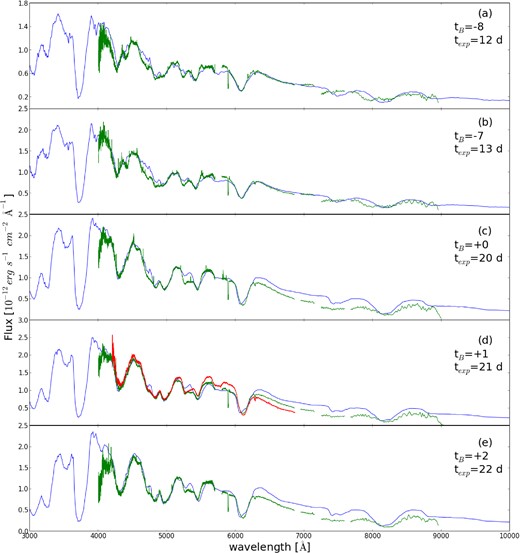
Modelled (blue) and observed spectra (green) of SN 2014J. Plot (a) is from −4 d, (b) is from −3 d, (c) is +0 d maximum, (d) is +1 d and (e) is +2 d. All of the dates are relative to B-band maximum. All spectra have been dereddened. The red spectrum at +1 d is from the INT.
There are strong Si ii 6355 Å, S ii 5454 Å and 5640 Å features. Due to this, the model requires a photospheric abundance of 12 per cent Si and 9 per cent S by mass, with 13 per cent Mg to produce the Mg ii 4481 Å line. The Mg ii 4481 Å line is the dominant line in the 4300 Å feature. The O abundance is 60 per cent and the Ca is 1 per cent. There are strong Ca ii features in this modelled spectrum, including a large absorption line in the H&K feature in the near UV (3934, 3968 Å). This absorption line is produced by our models in a strength consistent with the HST data (Foley et al. 2014). Although we do not cover this UV Ca line in our observations, we do have the Ca ii IR triplet from which we can infer the Ca abundances. The photospheric Ca ii IR triplet is modelled successfully, but there is no attempt to model the high-velocity feature. An iron abundance of 4 per cent is required to produce the Fe iii 5150 Å absorption line. The 56Ni abundance is at 0 per cent, because the ejecta at this epoch are still in the high-velocity outer layers of the photosphere. Ti+Cr are at a photospheric abundance of 0.3 per cent by mass. There is a low abundance of C at this high velocity as there are no C spectral features in the optical data, suggesting that all the carbon may be in earlier time spectra, although Marion et al. (2014) do find C i at 1.0693 μm. However, if we add C into the models we find this produces deeper and wider C absorption lines. Therefore, the C found in the NIR could be due to a very small abundance. There is a small absorption line in the optical observed at ∼6200 Å, where one would expect C, however this line is too narrow and not a C feature. The model at this epoch produces a particularly good match for the Fe ii/Mg ii 4200 Å, S ii 5640 Å and Si ii 6355 Å features.
6.2 Day −7
The second spectrum was taken −7 d from B-band maximum, texp = 13 d. The luminosity at this epoch is 109.408 L⊙ and vph = 11990 km s−1. There is very little variation between the first two epochs as they are only taken 1 d apart. The main chemical changes from the previous epoch are that Si has increased to a photospheric mass abundance of 15 per cent and S to 10 per cent. The 56Ni has also increased to 3 per cent. The ∼4200 Å feature is predominately Mg ii 4481 Å with smaller contributions from Fe iii 4419 Å. The Mg abundance is 10 per cent and the O abundance has decreased to 56 per cent. The Si iii 4550 Å line is successfully modelled, and this is the last FRODOSpec spectrum with a prominent Si iii feature.
6.3 Day +0
The third spectrum was taken on the night of B-band maximum, texp = 20 d (refer to Fig. 6). The luminosity is 109.455 L⊙ and photospheric velocity vph = 9480 km s−1. The Si and S abundances have increased relative to the previous epoch to photospheric mass abundances of 17 and 12 per cent, respectively, and the 56Ni has stayed constant at 3 per cent. 56Fe has also increased by 2–6 per cent. Conversely, the Mg and O abundances have decreased to 5 and 55 per cent, respectively. There is now a notable excess in flux in the red side of the spectrum due to the blackbody approximation. The B-band modelled absolute unreddened magnitude is −18.79. At this epoch, the modelled Si iii 4550 Å absorption line is not as strong as the previous epochs. Furthermore, in the previous spectrum the 4800 Å feature which have dominant Si ii 5056 Å and Fe ii 5169 Å absorption lines are merged into one, whereas at this epoch they have two distinct minima. Ca absorption is now more prominent in both the model and the observations, and is seen in the Ca ii IR triplet at ∼8200 Å.
6.4 Day +1
The next spectrum in the series was observed on +1 d relative to B-band maximum, texp = 21 d. It has a luminosity of 109.460 L⊙ and a photospheric velocity of vph = 8970 km s−1. This spectrum is at maximum bolometric luminosity, which is consistent with it being between B-band and V-band maximum. Although the INT and LT spectra differ slightly, predominantly in the red side of the spectrum, the main absorption lines in the blue side of the optical are similar between the spectra. Due to this, the abundances obtained in our analysis would not change if we were to model just the INT or LT spectra. The abundances we derive from this spectrum are very similar to the previous epoch; the Si decreases to 15 per cent, the S to 10 per cent the O to 57 per cent. 56Ni has increased to 11 per cent and 56Fe is constant at 6 per cent. The effective temperature at this epoch is 9000 K, which is 200 K lower than the previous spectrum. The Mg abundance has decreased to 0 per cent. The S ii 5454 Å feature is not as strong in the model as the observed spectrum; however, increasing S abundance would enhance the S ii 5640 Å line. There is excess strength of O i and Mg ii at 7773 and 7896 Å which could be an indication that there is excess mass at this velocity. This feature occurs in most of the epochs in the model, and is more dominant in late-time spectra.
6.5 Day +2
The fifth spectrum was observed on texp = 22 d (see Fig. 6). Its luminosity is 109.430 L⊙ and photospheric velocity is vph = 8440 km s−1. The effective temperature is 8900 K. The abundances at this epoch are very similar to the previous one, except for 56Ni which begins to increase dramatically to 36 per cent, S which decreases to 4 per cent; Si and O also decrease to 10 and 43 per cent, respectively. At this epoch, Ca stays constant at 2 per cent. The B-band unreddened modelled absolute magnitude of this spectra is −18.85. At this epoch the ∼4200 Å feature is still dominated by the Fe iii 4419 Å and Mg ii 4481 Å lines.
6.6 Day +3
The next spectrum was observed on texp = 23 d (refer to Fig. 7). The luminosity at this epoch is 109.390 L⊙, the photospheric velocity is vph = 7930 km s−1, the effective temperature is 7900 K and the B-band modelled absolute magnitude is −18.622. The modelled S ii 5640 Å feature is stronger than the observed one; this is a problem which consistently occurs in the model. To make the S ii the same strength as the observed one it would require the abundance of S to be reduced in the early-epoch models. However, we have chosen to fit the early-time spectra rather than the late-time ones, as these can lead us to more information about the high-velocity abundances. At this epoch, the O has a photospheric abundance of 0 per cent. The Si and S have also decreased to an abundance of 4 and 2 per cent by mass, respectively. The Fe ii 4420 Å and Si ii 6355 Å lines are modelled successfully. The wide deep absorption line at 8200 Å is the Ca ii IR triplet absorption line, the calcium has been reduced to a 1 per cent by mass to decrease the strength of this line. At this epoch 56Ni begins to dominate and is at 88 per cent. Given the sudden jump in the 56Ni abundance, we can give the constraint that the 56Ni distribution will extend to ∼8000 km s−1. We thus predict that the characteristic line width of the iron emission in the nebula spectra will be of the order of ∼8000 km s−1 (Mazzali et al. 1998).
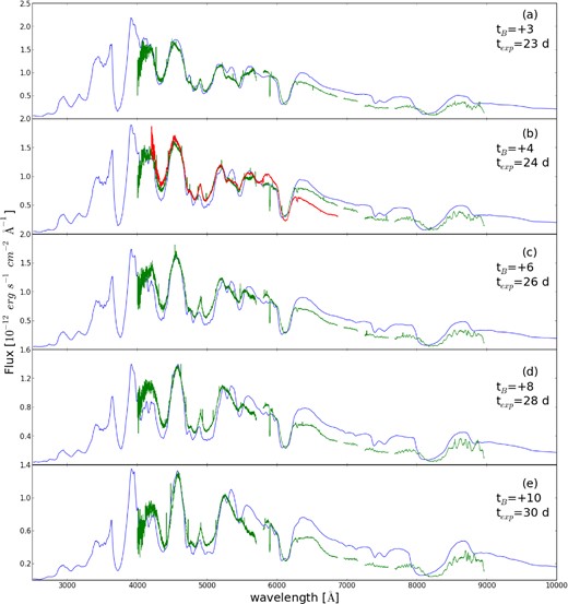
Modelled (blue) and observed spectra (green) of SN 2014J. Plot (a) is from +3 d, (b) is from +4 d, (c) is +5 d, (d) is +6 d and (e) is +8 d. All of the dates are relative to B-band maximum. All spectra have been dereddened. The red spectrum of +4 d is from the INT.
6.7 Day +4
The spectrum from +4 d has a luminosity of 109.345 L⊙ and photospheric velocity of vph = 7480 km s−1. There is a similar discrepancy between the INT and LT data as in the +1 d plot; however, once again this does not affect the abundances we obtain from our fits. From this epoch, the absorption lines are beginning to be stronger than the observed ones. For example, the modelled Fe/Mg 4300 Å and Fe 4800 Å features, which are produced by dominant Fe iii 4419 Å and Fe ii 5018 Å absorption lines. However, to refine this fit requires the abundances of these lines at high-velocity epochs to be reduced, affecting the early-time spectra. Therefore, we suggest that the excess absorption could be due to too much mass at vph = 7480 km s−1. Part of the excess in strength of the 56Fe lines could also be due to the decay of 56Ni. Due to this excess strength in Fe, its photospheric abundance is now at 0.1 per cent. The Si and S abundances have decreased to 0 per cent, and the 56Ni is at 99 per cent. The effective temperature at this epoch is 8600 K.
6.8 Day +6
The eighth spectrum was taken 26 d after explosion. It has a luminosity of 109.32 L⊙, a photospheric velocity of vph = 6500 km s−1 and an effective temperature of 8400 K. The 56Ni photospheric abundance is at 99 per cent. The Fe ii 4340 Å, S ii 5606 Å and Fe iii 4419 Å absorption lines are much deeper in the model than the observations. The unreddened modelled B and V magnitudes are 9.5 and 9.1 mag, respectively.
6.9 Day +8
The next spectrum has a luminosity of 109.250 L⊙ and photospheric velocity is vph = 5950 km s−1. The 56Ni abundance has stayed constant. The difference between the model and observation begins to differ even more, as shown by the Fe ii 4549 Å line in the 4800 Å feature. At this epoch, there is a significant amount of 56Ni above the photosphere. Therefore, it is not unexpected that the difference between the models and observed spectra begins to increase.
6.10 Day +10
The final epoch that was modelled is from +10 d from B-band maximum. It has a luminosity of 109.22 L⊙, a photospheric velocity of vph = 5450 km s−1 and an effective temperature of 7800 K. At this epoch there is no Si or S abundance, and the 56Ni abundance is the most dominant, at almost 100 per cent. The Ca abundance has now decreased to 0 per cent.
7 ABUNDANCE STRATIFICATION
We produce an abundance tomography distribution plot for the photospheric layers of the ejecta, see Fig. 8. This plot demonstrates how the abundances in the early times, from −8 to +10 d, of SN 2014J develops. We cannot definitively confirm the abundances of the outermost layers of the ejecta as we do not have spectra before −8 d. The abundances in the outer shell are slightly unusual, in that there is no carbon abundance. The other notable abundance is Fe which begins at 0.1 per cent and rises to 6 per cent. We have attempted to increase this, but doing so dramatically strengthens the Fe 4800 Å feature at all epochs. Therefore, the initial abundances of the outer shell, which has a velocity of 14 800 km s−1, are Si 10 per cent, O 78 per cent, S 4 per cent, 56Ni 0 per cent, Mg 7 per cent, C 0.0 per cent and 56Fe 0.1 per cent, with heavier elements making up the remaining abundance.

The abundance distribution of SN 2014J. The Ni/Co/Fe abundances are given in terms of mass fractions of 56Ni (56Ni0) and stable Fe (Fe0) at t = 0. In the spectral models no stable Ni or Co and no radioactive Fe is assumed to be present.
At high velocities, between 8440–14800 km s−1, there is a large oxygen abundance which starts at 78 per cent. The Si distribution starts at 10 per cent due to the strong Si ii 6355 Å feature, and it increases to 17 per cent at 9480 km s−1 before it decreases to 0 per cent at 7480 km s−1. Sulphur also follows a similar distribution with respect to velocity, although it always has a smaller abundance than Si. The sulphur distribution starts at 3.5 per cent before peaking at 12 per cent. The basic abundance evolution of the ejecta involves O dominating followed by the Intermediate Mass Elements (IME) and then by the heavy elements. In the abundance distribution plot, Fig. 8, the Fe starts at 0.1 per cent and rises to 6 per cent. In Fig. 8, the IME elements are significant at high velocities. From this, it can be inferred that the lighter elements may be at even higher velocities. Therefore, earlier spectra are needed to gain information about these lighter elements. As expected from a normal SN Ia explosion 56Ni dominates the abundance. This happens between 8440–7930 km s−1, where the 56Ni goes from a photospheric mass fraction of 36 to 83 per cent. The Ti+Cr abundances stay at a constant level throughout the whole explosion at 0.3 per cent. Calcium starts at 2 per cent at 12 300 km s−1 and it decreases to 1 per cent at 5450 km s−1.
The integrated abundances of the most important elements in the photospheric ejecta, which is at a velocity above 4400 km s−1, are M(Mg) = 0.07 M⊙, M(Fe) = 0.03 M⊙, M(O) = 0.40 M⊙, M(S) = 0.058 M⊙, M(Si) = 0.09 M⊙ and M(56Ni) = 0.47 M⊙. When the nebular phase spectra is available, the 56Ni could increase to a total integrated abundance of 0.72 M⊙. The final total integrated abundances can be confirmed when late-time spectra of SN 2014J are observed. Due to ground-based telescopes not being able to observe the UV part of the spectra, the iron-group element abundances of SN 2014J we have given here may show some 20 per cent uncertainty (of the values given), which nebular modelling will allow us to approve upon.
SN 2011fe and SN 2014J are photometrically similar. SN 2011fe has been used to determine the extinction of SN 2014J (Amanullah et al. 2014), and it has also been modelled using the same MC radiative transfer code (Mazzali et al. 2014). The total 56Ni abundance of SN 2011fe (Mazzali et al. 2014) and SN 2014J are very similar (0.4–0.7 M⊙ and 0.47–0.72 M⊙, respectively; the large range is due to not knowing abundance distribution in the nebula phase). Furthermore, the abundances in the photospheric region of the SN 2011fe ejecta are remarkably similar to those of SN 2014J. Changing the density profile in the models is not likely to qualitatively affect the abundance pattern in the regions of the ejecta explored by the spectra.
8 SUMMARY
We have presented photometric and spectroscopic observation of the closest SN Ia in at least the last 28 yr, SN 2014J. The observations were obtained with the LT and INT. We have presented SDSS g′r′i′ light curves and a spectral time series evolution over 12 epochs from −8 to +10 d, relative to B-band maximum. All of the spectra were calibrated in flux and atmospheric absorption lines were removed. The spectra show a very deep Si ii 6355 Å line and a Ca high-velocity feature at ∼7900 Å. We obtain a Δm15(B) = 0.88 ± 0.08 or 0.95 ± 0.12 using the g′ and r′ band or r′ band, respectively, and by fitting them through sifto. When correcting for reddening, this produced values of Δm15(B) = 0.98 ± 0.08 or 1.05 ± 0.12, respectively, using the SN 2011fe spectra, and Δm15(B) = 0.95 ± 0.08 or 1.02 ± 0.12 for the Hsiao template. This result is consistent with those of Foley et al. (2014). We obtain a Vmax of 10.66 ± 0.02.
SN 2014J is a highly reddened SN Ia which does not follow the conventional Galactic reddening law (RV = 3.1). We adopt the CCM law with a foreground galactic value of E(B − V) = 0.05 (RV = 3.1) and host galaxy extinction of E(B − V) = 1.2 (RV = 1.38). SN 2011fe and SN 2014J were found to have comparable Ni masses, 0.4–0.7 and 0.47–0.72 M⊙, respectively, when modelled using the same MC radiative transfer code. However, due to their difference in uncorrected decline rate we could expect these values to change. This could be revealed with the use of the UV data and the nebular spectra.
The spectra were modelled with the abundance tomography technique of Stehle et al. (2005), simulating spectrum formation with an MC radiative transfer code. The density profile used for this was W7. In follow-up papers, we will change the density structure in an attempt to refine the model.
The spectra were modelled at 10 epochs, before and after B-band maximum, inferring a best-fitting abundance stratification. As one would expect, at higher velocities (12 400 km s−1) there is a large abundance of oxygen. As the photosphere recedes (8440 km s−1) the IME elements dominate, Si and S. Then at low velocities the radioactive Ni dominates below 8000 km s−1. This leads to the prediction that the characteristic line width of the iron emission line in the nebular spectra will be of the order of 8000 km s−1 (Mazzali et al. 1998).
Synthetic spectra reproduce the spectral evolution of SN 2014J, and the final integrated abundances of SN 2014J are M(Mg) = 0.07 M⊙, M(Fe) = 0.03 M⊙, M(O) = 0.40 M⊙, M(S) = 0.05 M⊙, M(Si) = 0.09 M⊙ and M(56Ni) = 0.47–0.72 M⊙. Our results are consistent with the current understanding of SN Ia reddening and early-time abundance distribution. The observation and modelling in this paper is of particular significance because of the close proximity of SN 2014J. Furthermore, SN 2014J is the typical example of a normal SN Ia, making our models a good basis for studying further objects.
SH is funded from a Minerva ARCHES award of the German Ministry of Education and Research (BMBF). We have used data from the NASA / IPAC Extragalactic Database (NED, http://nedwww.ipac.caltech.edu, operated by the Jet Propulsion Laboratory, California Institute of Technology, under contract with the National Aeronautics and Space Administration). For data handling, we have made use of various software packages (as mentioned in the text) including iraf (Image Reduction and Analysis Facility). iraf (http://iraf.noao.edu) is an astronomical data reduction software distributed by the National Optical Astronomy Observatory (NOAO, operated by AURA, Inc., under contract with the National Science Foundation).
NASA/IPAC Extragalactic Database (NED).
iraf is distributed by the National Optical Astronomy Observatories, which are operated by the Association of Universities for Research in Astronomy, Inc., under cooperative agreement with the National Science Foundation.
