


Abstract
We investigate the scale dependence of fluctuations inside a realistic model of an evolving turbulent H ii region and to what extent these may be studied observationally. We find that the multiple scales of energy injection from champagne flows and the photoionization of clumps and filaments leads to a flatter spectrum of fluctuations than would be expected from top-down turbulence driven at the largest scales. The traditional structure function approach to the observational study of velocity fluctuations is shown to be incapable of reliably determining the velocity power spectrum of our simulation. We find that a more promising approach is the Velocity Channel Analysis technique of Lazarian & Pogosyan (2000), which, despite being intrinsically limited by thermal broadening, can successfully recover the logarithmic slope of the velocity power spectrum to a precision of ±0.1 from high-resolution optical emission-line spectroscopy.
1 INTRODUCTION
The line broadening in excess of thermal broadening seen in optical spectroscopic studies of H ii regions has been attributed to turbulence in the photoionized gas. There are many examples in the literature of attempts to identify the presence of and characterize this turbulence, for example Münch (1958), Roy & Joncas (1985), O'Dell & Castañeda (1987), Miville-Deschênes, Joncas & Durand (1995), Medina Tanco et al. (1997), Lagrois & Joncas (2011) and references cited by these papers. In these studies, the variation of the point-to-point radial velocities with scale was investigated using structure functions following von Hoerner (1951).
A general finding of these studies is that the structure function derived from these observations does not follow that predicted by Kolmogorov's law (Kolmogorov 1941). The interpretation of this result is that Kolmogorov's law for incompressible and subsonic turbulent flows cannot be strictly applied to the photoionized gas in H ii regions, which will be compressible and possibly mildly supersonic (Roy & Joncas 1985), or that energy does not cascade from larger to smaller scales but is input at many scales (Castañeda 1988). Moreover, the results differ according to which emission lines are used in the study, since the topology of the emitting gas will be different. For instance, the [O iii] λ5007 line comes from gas in the interior of an H ii region, whereas the [S ii] λ6731 line comes from the vicinity of the ionization front, essentially a two-dimensional surface. The suggested mechanisms responsible for the generation and maintenance of the turbulent velocities in H ii regions include photoevaporated flows from globules (Dyson 1968; O'Dell & Castañeda 1987) and stellar winds (Medina Tanco et al. 1997; Lagrois & Joncas 2011).
In order to construct the structure functions for the velocity fields, observations at many points in an H ii region are needed. This can be achieved either by multiple longslit spectroscopic observations at many positions across a nebula (Castañeda & O'Dell 1987; O'Dell, Townsley & Castañeda 1987; Wen & O'Dell 1993), or by Fabry–Perot interferometry (Roy & Joncas 1985; Miville-Deschênes et al. 1995; Lagrois et al. 2011). Longslit observations with high velocity resolution have enabled several velocity components to be identified for emission lines of metal ions for which the thermal widths are small, e.g. [O iii] λ5007. These observations have been used to determine the radial velocities of the principal components of the emitting gas at hundreds of positions within the nebula. Fabry–Perot observations produce data sets of thousands of radial velocities, but without the velocity resolution to distinguish between different velocity components. Obviously, in order to obtain a structure function over a wide range of scales, very high quality data with an ample spatial coverage are required. In the case of longslit spectra, this is a non-trivial task, not least the calibrating of the positions of the slits (García-Díaz & Henney 2007; García-Díaz et al. 2008).
Chandrasekhar (1949) suggested that turbulence is ubiquitous in astrophysics and that it could be analysed statistically via the spectrum of the velocity field, which expresses the correlations between instantaneous velocity components at all possible pairs of points in the medium. Turbulence develops in a fluid when velocity advection is dominant over dissipation (high Reynolds number), then continuous injection of energy is required in order to maintain the turbulent state. One of the main assumptions of the Kolmogorov theory of turbulence is that energy is only injected at large scales and is dissipated only at small scales. This implies that the energy cascades from large to small scales without dissipation. Another assumption of this theory is that in the range between injection and dissipation scales the energy is transferred at a constant rate, and this range is called the inertial range. Turbulence is often described in terms of the energy spectrum E(v), and the inertial range is represented by a power-law relationship E(v) ∝ kβ, where k is the wavenumber. For incompressible, homogeneous, isotropic, 3D turbulence (Kolmogorov 1941), we have β = −5/3, while in the limit of high Mach number, shock-dominated turbulence in one dimension (Burgers 1974), the power law is β = −2. It has proved more difficult to obtain exact results for the general case of 3D compressible, hydrodynamic turbulence. Scaling laws suggest that the original Kolmogorov energy spectrum scaling should be preserved even for highly compressible turbulence if the density weighted velocity ρ1/3v is taken instead of the pure velocity v (Kritsuk et al. 2007; Federrath et al. 2010). Recent work by Galtier & Banerjee (2011) predicts the relation E(ρ1/3v) ∝ k−19/9 for compressible, isothermal turbulence with compressive driving, with a turnover around the sonic scale to E(ρ1/3v) ∝ k−5/3. This has been confirmed by extremely high-resolution numerical experiments (Federrath 2013).
Another important prediction of the Kolmogorov theory is the scaling of the structure function of any order. The universality of such scaling laws has been tested by detailed numerical experiments (Boldyrev, Nordlund & Padoan 2002; Porter, Pouquet & Woodward 2002; Kritsuk et al. 2007; Federrath 2013). Even in numerical experiments of incompressible, homogeneous and isotropic turbulence with energy injection at a fixed large scale, it is found that the exponents of the higher order structure functions have an anomalous behaviour, which has been interpreted as the result of spatial and/or temporal intermittency. Intermittency is a sparseness in space and time of strong structures associated with the dissipation or injection of energy (She & Leveque 1994). Since astrophysical turbulence driven by real physical phenomena is almost certainly intermittent, it is important to understand the possible effects of intermittency on the derived statistical properties of real H ii regions.
The three-dimensional properties of the density and velocity fields that describe the turbulence in the interstellar medium, in this case an H ii region, must be deduced from the statistical properties of the observed quantities. For photoionized gas, the observations generally consist of spectra at different positions, from which centroid velocities and linewidths can be obtained. For optical line emission, the emissivity depends on density, temperature and ionization state and therefore an analysis of the emission lines will not just be providing information on the turbulent velocity fluctuations in the gas. The observations are a two-dimensional projection of the three-dimensional properties and much effort has been dedicated to the problem of recovering 3D information from 2D data (Lazarian & Pogosyan 2000; Brunt & Heyer 2002; Miville-Deschênes, Levrier & Falgarone 2003; Brunt & Mac Low 2004; Esquivel & Lazarian 2005; Brunt, Federrath & Price 2010). Generally, some simplifying assumptions, such as isothermal gas and statistical isotropy of the turbulence, must be made.
Recent modelling of H ii regions has addressed the origin of the irregular structures, filaments, and globules seen within and around the borders in optical images (García-Segura & Franco 1996; Williams, Ward-Thompson & Whitworth 2001; Mellema et al. 2006b; Mackey & Lim 2010; Arthur et al. 2011). Morphologically, the simulated emission-line images are very reminiscent of observed H ii regions and the global dynamics, as measured by the rms velocity, is also similar to observationally derived values (García-Díaz et al. 2008; Arthur et al. 2011; Lagrois et al. 2011). The internal dynamics of the simulated H ii regions is due mainly to the interaction of photoevaporated flows from the heads of the filaments and clumps, which flow into the interior of the H ii region, superimposed on the general expansion of the H ii region (Mellema et al. 2006b; Lagrois et al. 2011). However, the dynamics of real H ii regions could also be affected at large scales by the action of stellar winds from the ionizing star or stars, and at small scales by outflows from young, low-mass stars.
In this paper, we investigate to what extent our numerical simulations of H ii regions model observed statistical properties of real H ii regions. In Section 2, we briefly describe the numerical methods used in the radiation-hydrodynamics simulations and in the calculation of the simulated emission-line radiation, and how the statistical information is obtained from these calculations. In Section 3, we describe our results for the expansion of an H ii region in a turbulent, clumpy molecular cloud. We discuss these results in Section 4, and comment on the extent to which the statistical properties of the numerical simulations agree with those of observed H ii regions. In Section 5, we summarize and present our conclusions.
2 NUMERICAL MODEL
We perform radiation-hydrodynamic simulations of the expansion of photoionized regions in a non-uniform initially neutral medium. The central ionizing source has an effective temperature of 37 500 K and an ionizing photon rate of 1048.5 s−1, which corresponds approximately to an O7 star.
The simulation takes as an initial condition a clumpy medium with mean density 〈n0〉 = 1000 cm−3, which results from a self-gravitating forced turbulence simulation by Vázquez-Semadeni, Kim & Ballesteros-Paredes (2005). The computational cube represents a spatial volume of 4 pc3 and the initial temperature is 5 K.
The radiation-hydrodynamics code used in this paper does not include self-gravity. However, although the initial conditions would be gravitationally unstable in the absence of photoionization heating, on the relatively short time-scales of the simulations (∼3 × 10⁵ yr) this will not be important since the global free-fall time of the computational cube is ∼6 × 10⁵ yr.
2.1 Radiation-hydrodynamics code
The radiation-hydrodynamics code used in this paper is the same as that used by Mellema et al. (2006b). The hydrodynamics is calculated using the non-relativistic Roe solver PPM scheme described in Eulderink & Mellema (1995) with the addition of a local oscillation filter (Sutherland, Bisset & Bicknell 2003) to suppress numerical odd–even decoupling behind radiatively cooling shock waves. Heating and cooling in the ionized and neutral gas is dealt with in the same manner as described in detail by Henney et al. (2009). The radiation transport and photoionization makes use of the c2-ray (Conservative-Causal ray) code developed by Mellema et al. (2006a). The calculations are all performed on a fixed, uniform Cartesian grid in three dimensions with a resolution of 5123 cells.
2.2 Simulated emission lines
The emissivity cubes for the Hα recombination line and the [O iii] λ5007, [N ii] λ6584 and [S ii] λ6731 collisionally excited lines are calculated as described in Arthur et al. (2011), with the assumption that the heavy element ionization fractions are fixed functions of the hydrogen ionization fractions, calibrated with the cloudy photoionization code (Ferland et al. 2013).
2.3 Turbulence statistics
The emissivity statistics have contributions from velocity, density, temperature and ionization state fluctuations. Obviously, the velocity fluctuations are the most dynamically important statistic and spectral line data, both real and simulated, can be used to extract statistical information for the different contributions. In particular, the second-order structure function of the velocity centroids and the technique of velocity channel analysis (VCA; Lazarian & Pogosyan 2000) have been widely used.
In this paper, we calculate the second-order structure function of the velocity centroids of the simulated emission lines and also apply VCA to the corresponding position–position–velocity (PPV) data cubes. In addition, we calculate the power spectrum of the velocity field, both weighted and unweighted, of the 3D hydrodynamic simulation data cube in an attempt to relate the observed statistics to the underlying hydrodynamics.
2.3.1 Power spectrum
Often the power spectrum can be represented by a power law p3(k) ∝ kn. For instance, the velocity field for incompressible, homogeneous (Kolmogorov 1941) turbulence has n = −11/3, while for shock-dominated turbulence (Burgers 1974), the 3D power-law index is n = −4.
2.3.2 Velocity centroid statistics
The use of positional fluctuations in the velocity centroids of spectral lines as probes of turbulent gas motions was developed in the 1950s by, for example, Münch (1958), and has been applied to observations of molecular emission lines in molecular cloud complexes (Dickman & Kleiner 1985; Kleiner & Dickman 1985) and to optical emission lines in the Orion nebula, Galactic and extragalactic H ii regions (Roy & Joncas 1985; O'Dell & Castañeda 1987; Castañeda 1988; Lagrois et al. 2011).
For homogeneous, incompressible (Kolmogorov) turbulence, the velocity fluctuations scale as l1/3 and hence the second-order structure function scales like l2/3. For isotropic velocity fields, the structure function and the autocorrelation function (see equation 1) have the same scaling and differ only by a constant. The structure function is therefore related to the power spectrum. If the power-law index of the 3D structure function is m, then the power-law index of the 3D power spectrum is n = −3 − m.
2.3.3 Velocity channel analysis
The relationship between the velocity centroids and the statistics of the velocity field is only reliable if the density fluctuations are negligible. VCA was developed to extract the separate contributions of density and velocity from spectral line data cubes.
This is a technique for analysing PPV cubes developed by Lazarian & Pogosyan (2000). With this method, spectroscopic observations are not reduced to velocity centroids as a function of position on the plane of the sky. Instead, the PPV cubes are analysed in terms of velocity channels, or slices, as a function of the velocity resolution used. As the width of the velocity slices increases, the relative contribution of a velocity fluctuation to the total intensity fluctuations decreases, because the contributions from many velocity fluctuations will be averaged out in thicker velocity slices. A slice is described as thick when the dispersion of turbulent velocities is less than the velocity slice thickness on the turbulence scale studied, otherwise the slice is thin (Esquivel et al. 2003). In the thickest velocity channels, we obtain only information about the density fluctuations, since the velocity information is averaged out. Conversely, the velocity fluctuations dominate in thin channels.
VCA consists of obtaining the 2D power spectrum for each velocity channel and then averaging over all velocity channels for each PPV cube. Esquivel et al. (2003) stress that whether a slice in velocity space is considered thin or thick depends not only on the slice width δv = (vmax − vmin)/N, where N is the number of channels, but also on the scale of the turbulence. For power-law statistics, the velocity dispersion scales as σr ∝ rm/2, where m is the velocity structure function index. The criterion for a channel to be considered thin is δv < σr, hence we do not expect a pure power-law result from the averaged 2D power-spectra analysis. This is because the largest scales, of the order of the size of the cube, are almost always in the thin regime. At the smallest scales, numerical dissipation plays a role, and there is an additional deviation from the power law.
2.3.4 Projection smoothing
The effect of projecting a three-dimensional correlation function on to a two-dimensional space has been studied by von Hoerner (1951), Münch (1958), O'Dell & Castañeda (1987) and Brunt & Mac Low (2004), among others. For the velocity field, the two-dimensional case corresponds to the emission-line velocity centroid map.
Previous authors have established that for an isotropic, power-law, three-dimensional power spectrum, the spectral index does not change on going from three dimensions to two (projected) dimensions, i.e. κ2D = κ3D, where κND is the power spectrum spectral index in N dimensions (defined as |$p_N(k) \propto k^{-\kappa _{N{\rm D}}}$|; Stutzki et al. 1998; Miville-Deschênes et al. 2003; Brunt et al. 2003). This is because the line-of-sight contribution to the line-of-sight velocity has no amplitude on the kz = 0 plane, where z is the line-of-sight direction.
The relationship between the power spectrum spectral index and the exponent of the second-order structure function for homogeneous turbulence is κND = mND + N, where mND is the power-law index of the N-dimensional second-order structure function. For projection from 3 to 2 dimensions, we therefore have m2D = m3D + 1, and this is known as projection smoothing.
In the case of incompressible, homogeneous (Kolmogorov) turbulence, we have κ3D = 11/3 and m3D = 2/3, hence the relationship κ2D = κ3D leads to m2D = 5/3. For the compressible turbulence (Burgers 1974) case, we have κ3D = κ2D = 4 and m3D = 1, leading to m2D = 2. When the line-of-sight depth is small compared to the plane-of-the sky size of the emitting region, the distribution of emitters is essentially two-dimensional (sheet-like) and we would expect m2D ≃ m3D (O'Dell & Castañeda 1987; Miville-Deschênes et al. 2003).
In order to compensate for the effects of density inhomogeneities, Brunt & Mac Low (2004) introduced a correction term δκ such that κ2D = κ3D + δκ, where δκ tends to −1 when density fluctuations are important. This idea was applied by Lagrois & Joncas (2011) in an effort to use 2D observational statistics to infer the 3D velocity field of photoionized gas in giant extragalactic H ii regions.
3 RESULTS
3.1 General properties
We begin by considering the morphological appearance of the simulated H ii regions. Fig. 1 shows the evolutionary sequence from 150 000 to 300 000 yr. Each image is a composition of the three optical emission lines [N ii] λ6584 (red), Hα (green) and [O iii] λ5007 (blue), where we have employed the classical Hubble Space Telescope red–green–blue colour scheme. Emission from the dense, neutral zones is negligible and for the production of these images we also include dust extinction in the radiative transfer for the projection to the plane of the sky, with the assumption that the dust-to-gas mass ratio is 1 per cent.
![Simulated projected emission-line images of an evolving H ii region in a turbulent molecular cloud. The panels show the H ii region at 150 000, 200 000, 250 000 and 300 000 yr, from top left to bottom right. The physical size of each image is 4 pc on a side and the resolution of the simulation is 5123 cells. The view is from the negative −z direction of the computational cube. The colours represent the optical emission lines [N ii] λ6584 (red), Hα (green) and [O iii] λ5007 (blue), and for these images the effect of dust absorption has been included in the radiative transfer during the projection on to the plane of the sky.](https://oup.silverchair-cdn.com/oup/backfile/Content_public/Journal/mnras/445/2/10.1093_mnras_stu1862/2/m_stu1862fig1.jpeg?Expires=1750737133&Signature=W3g3z4-tlK5bnxeGiLE7gMhbeSVmiyIJ0L8Pl~yfMybVa8T9xPx9Jzm84pVM-X9GPleb1Mj7D7IR4rNtmZ9GufyOLs1KAcq-kFGKhsvbnnW8dcKaFdeDaHhCUoxZDNv~Jp9wpthbOlx83ryPF9gQB3wRQIdFqc6nd3zMbfBKlpqPUF0cgTuiTtea55bqRD103AH837lqWL7IYrdppffwsKcH5pmaS1g-4-ODkzE9xTot-5PbDm2-mA3l6x2bu2lr~ZmS-SrJrME0syQkGDP6XPOdGp6MQU89PNumDB6YVeNK4NBggWtNyIZLYTKavbNIlj0M2ITt8EOcxl6ixzGpag__&Key-Pair-Id=APKAIE5G5CRDK6RD3PGA)
Simulated projected emission-line images of an evolving H ii region in a turbulent molecular cloud. The panels show the H ii region at 150 000, 200 000, 250 000 and 300 000 yr, from top left to bottom right. The physical size of each image is 4 pc on a side and the resolution of the simulation is 5123 cells. The view is from the negative −z direction of the computational cube. The colours represent the optical emission lines [N ii] λ6584 (red), Hα (green) and [O iii] λ5007 (blue), and for these images the effect of dust absorption has been included in the radiative transfer during the projection on to the plane of the sky.
The images show that the ionized gas distribution is not spherical and around the corrugated edge of the H ii region there are many neutral clumps and fingers of gas. This is a consequence of the H ii region evolving in a clumpy neutral medium. The fingers and clumps at the edge of the H ii region are the remnants of denser regions in the initial turbulent cloud. We can also see that the different ions are important in different regions of the photoionized gas. The [O iii] λ5007 (blue) emission is strongest closer to the photoionizing source, while the [N ii] λ6584 (red) emission is most prominent around the edge of the H ii region and the Hα is distributed throughout the nebula. Although not shown in Fig. 1, we also calculate the [S ii] λ6716 emission, which is important only around the edge of the H ii region in the vicinity of the ionization front. This is consistent with the phenomenon of ionization stratification (Osterbrock & Ferland 2006).
The neutral clumps and fingers around the edge of the H ii region are the source of photoevaporated flows, which flow away from the ionization front into the H ii region (Henney 2003). These flows are mildly supersonic and can reach velocities of up to two or three times the sound speed in the ionized gas. They shock against each other in the interior of the H ii region. Neutral clumps inside the H ii region are accelerated outwards by the rocket effect in the opposite direction to the photoevaporated material flowing off their ionized skins. In Fig. 1 these photoevaporated flows can be discerned as shadowy regions ahead of the convex bright cusps that mark the position of the ionization front. As the photoevaporated gas flows away from the ionization front, the density drops in the diverging flow and this is why the flows appear darker than the surrounding photoionized gas.
These colliding photoevaporated flows are responsible for the velocity dispersion of the ionized gas, which we show in Fig. 2. This figure shows both the mass-weighted velocity dispersion of the ionized gas and the volume-weighted velocity dispersion. At early times (t < 105 yr), the volume-weighted velocity dispersion is higher than that of the mass-weighted velocity dispersion. This is because the H ii region breaks out of the dense clump where it is formed after about 50 000 yr and a low-density, relatively high-velocity champagne flow results. After about 100 000 yr, the main ionization front has just about caught up and thereafter the two different velocity dispersions show the same behaviour, remaining roughly constant with Vrms ∼ 8 km s−1. In Fig. 2, we also show the rms velocity for the analytical expansion (Spitzer 1978) in a uniform medium, where the gas velocity behind the ionization front is one half that of the ionization front and the internal velocities are linear with radius. In this case, the velocity dispersion falls steadily as a function of time, and after 100 000 yr is less than 2 km s−1. The differences between the velocity dispersions in the numerical and analytic cases are mainly due to the interaction of the photoevaporated flows produced in the simulations described above. In the analytic expansion, the velocities are radial away from the central source. In the clumpy medium, the photoevaporated flows lead to large non-radial velocities, which increase the velocity dispersion in the photionized region. Finally, Fig. 2 also shows that the mass-weighted mean radial velocity peaks just before 200 000 yr at about 7 km s−1 and thereafter falls off. This indicates that the global expansion will not be an important influence on the dynamics, compared to the velocity dispersion, after 200 000 yr.

Velocity dispersion as a function of time. The thick, black solid line shows the mass-weighted velocity dispersion of the ionized gas, the dotted line is the volume-weighted velocity dispersion of the ionized gas, while the thick grey line is the rms velocity of the analytical expansion (Spitzer 1978) in a uniform medium of density n0. The thin, black continuous line is the mass-weighted mean radial expansion velocity of the ionized gas.
In Fig. 3, we compare the sound-crossing time of the ionized volume with the evolution time of the simulation. During the breakout of the H ii region from its initial dense clump (between about 80 000 and 100 000 yr), the expansion is supersonic and the sound-crossing time exceeds the evolution time. This coincides with the peak in the velocity dispersion (see Fig. 2). After this time, the expansion is subsonic and the sound-crossing time becomes shorter than the evolution time. A statistically steady state then becomes possible for the turbulence within the ionized volume.
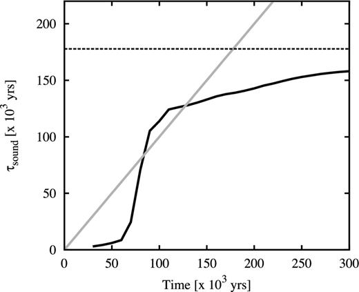
Sound-crossing time as a function of evolution time. The sound-crossing time is 〈R〉/ci, where 〈R〉 is the radius of an equivalent sphere with volume equal to that of the H ii region and ci = 11 km s−1 is the sound speed in the photoionized gas. The diagonal grey line has slope of unity. The horizontal dashed line is the sound-crossing time for a distance of 2 pc, which is the half-side length of the computational box.
3.2 Statistical properties
3.2.1 Power spectra
In Fig. 4, we show the 3D power spectra of the ionized gas velocity, the ionized density and the ionized velocity weighted by the cube root of the density (see e.g. Kritsuk et al. 2007). In the following sections, we use a dimensionless k that is normalized to the size of our computational grid. Thus k = 1 corresponds to a physical scale of 4 pc. The power spectra all exhibit a break in the power law at about wavenumber k ∼ 32, equivalent to a scale of 16 computational cells and consistent with the numerical dissipation scale. We fit power laws between k = 4 (corresponding to a length-scale of 1 pc) and k = 32. For times later than 200 000 yr, the power-law fits for a given quantity are essentially constant (see Fig. 5). Note that here we use n to represent the 3D power spectrum spectral index,1 which corresponds to the slope or gradient in log–log space, where n = −κ3D and κ3D is defined in Section 2.3.4. At earlier times, the power laws are steeper and evolving. The settling down of the power spectra power-law indices correlates with the time at which the global expansion ceases to be important for the internal dynamics (see Fig. 2). This occurs after about 200 000 yr (as evidenced in Fig. 5), which corresponds to the evolution time being equal to approximately 1.5 times the sound-crossing time (see Fig. 3).

Power spectra of the 3D simulation cube. From top to bottom: ionized gas velocity vi, ionized gas density di, ionized gas velocity weighted by the cube root of the density |$v_{\rm i} d_{\rm i}^{1/3}$|. From left to right: 150 000, 200 000, 250 000 and 300 000 yr. The points represent the calculated power spectra for the numerical simulation and the solid line is the least-squares fit to the data points between limits described in the text, represented by the grey rectangle. The index n of each power-law fit is indicated in the corresponding panel.
![Time variation of 3D power spectra power-law indices. Top panel: 3D physical quantities; solid line – ionized gas velocity vi, dashed line – ionized density di, dotted line – square of ionized density $d_{\rm i}^2$, dot–dashed line – temperature T. Bottom panel: emission-line volume emissivities; filled circles – j(Hα), open squares – $j(\mathrm{[O\,\small {III}]})$, filled triangles – $j(\mathrm{[N\,\small {II}]})$, open diamonds – $j(\mathrm{[S\,\small {II}]})$.](https://oup.silverchair-cdn.com/oup/backfile/Content_public/Journal/mnras/445/2/10.1093_mnras_stu1862/2/m_stu1862fig5.jpeg?Expires=1750737134&Signature=sTBfBvpSiXUipFc0bJfnBJJoWpN31zCQQcHbnMBJ6bSSyvkNC-rqMSBHjTHV5t5d~OsGBpDRJ7njg7kSFQTJGwGcpk1Nzrqr3MS3mkkX8T86~isev7Cs~m5I3QLIj-jl-JCxkpYzgQZCc-H009DIH8u4J-wB20ZY97qWx7RT5DA-F8CtcM3fKs8FazRU5OqK5RSQc3KcoZI11nqgQ966BGkuPXugQw42tM~SIKUJ1FdsZkV7XZjt8AACALy6WkVlKV2Qm~Z-OX~ijEHHK6UT6wKBx3tRVk2PGWy7L8wglkChHYb-b8Y7CkXbaewSw-DgnMxneJTFDyKDEUK~u~eXBg__&Key-Pair-Id=APKAIE5G5CRDK6RD3PGA)
Time variation of 3D power spectra power-law indices. Top panel: 3D physical quantities; solid line – ionized gas velocity vi, dashed line – ionized density di, dotted line – square of ionized density |$d_{\rm i}^2$|, dot–dashed line – temperature T. Bottom panel: emission-line volume emissivities; filled circles – j(Hα), open squares – |$j(\mathrm{[O\,\small {III}]})$|, filled triangles – |$j(\mathrm{[N\,\small {II}]})$|, open diamonds – |$j(\mathrm{[S\,\small {II}]})$|.
3.2.2 Second-order structure functions
We use the procedure described in Section 2.3.2 to calculate velocity centroid maps for the Hα, [O iii] λ5007, [N ii] λ6584 and also [S ii] λ6716 emission lines and then calculate the corresponding second-order structure functions according to equation (4). Results for representative evolutionary times are shown in Figs A1 –A3 of Appendix A, where fits to the power-law index (m2D) of the structure function, which corresponds to the slope or gradient in log–log space, are carried out for the inertial range of scales. A description of the procedure for identifying the inertial range is given in Appendix A and illustrated by the accompanying Fig. A4.
In Fig. 6, we show the evolution of m2D with time for the different lines and for the three principal viewing directions of the simulation cube. For the line of sight along the z-axis (first column of Fig. 6), one sees for all lines a consistent steepening of the structure function graph with time (increase in m2D). But for other viewing directions no such trend is apparent: both rising and falling behaviour of m2D is seen, with little consistency between different lines.
![Evolution of second-order structure function power-law index, m2D, as a function of time. From top to bottom: Hα, [O iii] λ5007, [N ii] λ6584, [S ii] λ6716. From left to right: line of sight along the z, y and x axes, respectively.](https://oup.silverchair-cdn.com/oup/backfile/Content_public/Journal/mnras/445/2/10.1093_mnras_stu1862/2/m_stu1862fig6.jpeg?Expires=1750737134&Signature=lBHG3aNJI80KJiOnMsApdnN2Lhpa0j7pheHJXDCJ74XLeJJ-ZixBGzXHU-z31xWubvj22QJss6kax0BXUdzLR8cW1j-Py5hqu~d-kcs8oYDLdFpv-EFPIWzXCnm7EWX3lXkQ0vKTZvSyziyWIzuraGXTKbyNAw5tLJ~miHR9K~jIfw0bF4Er-NaEg4BLfQy86jo~PHpyM4ZCJZu1cdyiPCh00Ncq4LjuR-cQOBH~EVAvF4twg12FZ8c4HQETHOoWVRdq2HxaauPF8tI2lsd7L-ls9GG1p3Ond-uiWd0w8NpHD9d5gmztAejfs3isrrfWdkD4GRRjgA9HPDuEmIjlBg__&Key-Pair-Id=APKAIE5G5CRDK6RD3PGA)
Evolution of second-order structure function power-law index, m2D, as a function of time. From top to bottom: Hα, [O iii] λ5007, [N ii] λ6584, [S ii] λ6716. From left to right: line of sight along the z, y and x axes, respectively.
In order to understand why one particular viewing direction is different, we produced histograms of the emission-line velocity centroid values binned into narrow <2 km s−1 bins for the three different lines of sight at the four different times. The histograms are presented in Fig. 7, from which we see that for the z-axis line of sight, the values of Vc are not distributed symmetrically about the mean value and, in fact, for the Hα and [O iii] λ5007 emission lines, a ‘wing’ develops for negative values of Vc that extends to more negative values as time progresses. This tendency is not seen for the y- and x-axis lines of sight. We attribute this wing to a ‘champagne’ flow towards the observer along the z-axis. This flow would be perpendicular to the line of sight for observations along the other axes.
![Histograms of velocity centroid values for each emission line along different lines of sight. From top to bottom: Hα, [O iii] λ5007, [N ii] λ6584, [S ii] λ6716. From left to right: line of sight along the z, y and x axes, respectively. The different line types refer to different times: thick, grey line – 150 000 yr, dashed line – 200 000 yr, short-dashed line – 250 000 yr, continuous black line – 300 000 yr.](https://oup.silverchair-cdn.com/oup/backfile/Content_public/Journal/mnras/445/2/10.1093_mnras_stu1862/2/m_stu1862fig7.jpeg?Expires=1750737134&Signature=xNlQ-ZKHAZWLxqraNtw1dgs3u4BoM2zB9uI1lAD6w7Npa24uN5gUV4a9nEs~Tru2K5uK9EM9muOCMMCsCTPdHvJfFmhRxgU7OtsdhTTWNMQ45xlcGqPLXOAMmFDpRVVKk~gwHOmb-2hUi81bOfy8NPTLoafJmKmC7ptY1fuAdQf-1d6MG4D4SOzJ34flW2UQGFoVNMYaondlD9WR~QkkvD1wFP7q-1JDTlLEaLvnHzX5-5ij6hjSodlCEEUfL3dwYb5flPuAsYHogV7wQWHHAyS1JC-8vFviUbwfC-aprKuqpYwaZuTVrgVlxz4TXxpPJ74wZhhyL3M5ghpnagD32Q__&Key-Pair-Id=APKAIE5G5CRDK6RD3PGA)
Histograms of velocity centroid values for each emission line along different lines of sight. From top to bottom: Hα, [O iii] λ5007, [N ii] λ6584, [S ii] λ6716. From left to right: line of sight along the z, y and x axes, respectively. The different line types refer to different times: thick, grey line – 150 000 yr, dashed line – 200 000 yr, short-dashed line – 250 000 yr, continuous black line – 300 000 yr.
3.2.3 Velocity channel analysis
The VCA consists of calculating the two-dimensional power spectrum of the brightness distribution in isovelocity channels of varying thickness. We consider two cases: thick slices, which are wide enough (∼100 km s−1) to include all the emission in the line, and thin slices, with width 5 km s−1. Because the velocity spectrum in our simulations is rather shallow (see above), the line-of-sight turbulent velocity dispersion δv exceeds the width of these thin slices over the full range of length-scales that we can usefully study, from 0.1 pc (δv ≈ 8 km s−1) to 1 pc (δv ≈ 10 km s−1). Fig. 8 shows typical examples of the [O iii] brightness in thick and thin slices.
![Surface brightness maps in thick (left) versus thin (right) velocity slices for the [O iii] line from our simulation at an age of 300 000 yr. The thick slice covers the full velocity range of the emission line, while the thin slice has a width of 5 km s−1, which is smaller than the turbulent velocity fluctuations, but slightly larger than the thermal broadening for this line. It is apparent that the thin slice shows considerably greater small-scale structure than the thick slice, which is reflected in its shallower power spectrum. The brightness structure in the thick slice is due entirely to the emissivity fluctuations within the H ii region, whereas the additional structure in the thin slice is caused by velocity fluctuations.](https://oup.silverchair-cdn.com/oup/backfile/Content_public/Journal/mnras/445/2/10.1093_mnras_stu1862/2/m_stu1862fig8.jpeg?Expires=1750737134&Signature=mtEYAAd9qsd8wp06DRaI21hBX8OlfHrpra5QJgi~DOz3ZkZFolJG~HBaDk7qJWlhmmT1-4caFsTWsVYd3M9BlIye2~l3FXnBhRq43avt6TvBayg3JG69Gujzckd4ZaxIetit2zCteV81qqcmfOcyU3DqYFfxaL9DjpOlu3k-e575h6nxUeDQvkhoPjAVNbma2sxZxaxRYGcTmY4v~N9kp5858LKe3~NKjGbmA97OgivpmMb~i0YjGnB62x9yn~jZJX8hMDUaRJK5Vyb1vGPcJ8LucLAYQjl6ifiqFY3L9MnkokQcwXSZLUrIZDJv~z-soXePstB4RIfpBQcPDiqLyQ__&Key-Pair-Id=APKAIE5G5CRDK6RD3PGA)
Surface brightness maps in thick (left) versus thin (right) velocity slices for the [O iii] line from our simulation at an age of 300 000 yr. The thick slice covers the full velocity range of the emission line, while the thin slice has a width of 5 km s−1, which is smaller than the turbulent velocity fluctuations, but slightly larger than the thermal broadening for this line. It is apparent that the thin slice shows considerably greater small-scale structure than the thick slice, which is reflected in its shallower power spectrum. The brightness structure in the thick slice is due entirely to the emissivity fluctuations within the H ii region, whereas the additional structure in the thin slice is caused by velocity fluctuations.
To use thinner slices would not be useful for a variety of reasons. First, 5 km s−1 corresponds to the highest resolution that can be achieved with optical spectrographs that are optimised for studying extended sources, such as Keck HIRES or VLT UVES. Secondly, thinner slices are increasingly subject to ‘shot noise’ due to the finite resolution of the numerical simulations, which produces spurious small-scale power, as discussed by Esquivel et al. (2003) and Miville-Deschênes et al. (2003). Thirdly, thermal broadening would smooth out any structure on scales <5 km s−1 for all but the heaviest ions.
Fig. 9 shows the evolution with time of the VCA power-law indices from thin (γt) and thick (γT) channels (shown by filled circle and cross symbols, respectively) for different ions and for different viewing directions. The individual VCA power spectra from which these power-law indices, which correspond to the slope or gradient in log–log space, were extracted are presented in Appendix B. It can be seen that both γt and γT are remarkably stable with time during the latter part of the evolution (t > 200 000 yr). Although thermal broadening means that there is no clear distinction between γt and γT for the Hα line, the two values are clearly distinguished for the heavier ions, with the thin slices showing a significantly shallower slope, especially for [O iii]. The implications for diagnosing turbulence statistics are discussed in Section 4.1.3.
![Evolution of velocity channel power-law index as a function of time for thick channels (γT; crosses) and thin channels (γt; filled circles). From top to bottom: Hα, [O iii] λ5007, [N ii] λ6584, [S ii] λ6716. From left to right: line of sight along the z, y and x axes, respectively. Thermal broadening was included in all cases.](https://oup.silverchair-cdn.com/oup/backfile/Content_public/Journal/mnras/445/2/10.1093_mnras_stu1862/2/m_stu1862fig9.jpeg?Expires=1750737134&Signature=2XiXAwX3tFZqIkXsH~Lwzv6xwG~9f6v84fmucMY2l-uKvgMEqaraUBGQUxwav8vbNbH8Ms3HTKlzX89hUdN3VNxCJ~kVmniYnCsBxKbtJhFTsAfmRbUxoD9cp-hhakZXD5-a0o5J~cDfj00axWmAjh-nLoElqErAtJsZfPzxIioZ2AnfaZ23O4~HRCqexhv98MjLhlmxAfkyrVar8L~b6ZLdbXUVbYX2csTqY1HMXy8CC-SPBvXeFUvz3i1VdMdmNurOuK~OersxeN~HPuiXrHoLTWwWQVksbtIFgzMakioOzfnalsweVPiK4iNsQN-4iymKJ6iurQgtdpcWMrv7AA__&Key-Pair-Id=APKAIE5G5CRDK6RD3PGA)
Evolution of velocity channel power-law index as a function of time for thick channels (γT; crosses) and thin channels (γt; filled circles). From top to bottom: Hα, [O iii] λ5007, [N ii] λ6584, [S ii] λ6716. From left to right: line of sight along the z, y and x axes, respectively. Thermal broadening was included in all cases.
4 DISCUSSION
4.1 Characterization of the turbulence from optical emission lines
At times later than 150 000 yr, our second-order structure function results for the Hα and [O iii] λ5007 emission-line velocity centroids strongly suggest the presence of turbulence with an inertial range between 1 pc and the numerical dissipation scale of about eight cells (equivalent to 0.0625 pc). The [N ii] λ6584 and [S ii] λ6716 structure function results also suggest turbulence, with a smaller upper limit to the inertial range, which is consistent with these ions being confined to relatively thin layers near the ionization front. However, it is difficult to characterize this turbulence since the slope of the structure function for a given emission line varies with time in an unpredictable manner and also depends on the line of sight. Although the results for the z-axis line of sight suggest an increase in slope with time, an examination of the distributions of the velocity centroids (see Fig. 7) shows that this is due to a champagne-type flow in that direction, and other lines of sight do not show a definite trend with time.
Different emission lines originate in different volumes of ionized gas, and this is reflected in the different slopes for the structure functions from different emitters. The Hα line is produced throughout the volume and is brightest close to the ionization front around the bright edges of the photoionized gas. There is therefore a wide range of densities associated with the Hα-emitting gas. The emissivity of the Hα recombination line depends on the square of the density and only weakly on the temperature in the photoionized gas (see e.g. Osterbrock & Ferland 2006). Indeed, the gradients of the 3D power spectra of the Hα emissivity and the square of the density are essentially the same. On the other hand, the emissivity of the [O iii] λ5007 collisional line depends more strongly on temperature. This line originates in the interior of the H ii region, where the density is more uniform but weak shocks due to the collision of photoevaporated flows cause fluctuations in the temperature. A more uniform density distribution corresponds to a steeper density power spectrum and, indeed, the structure functions, 2D velocity channel power spectra and 3D power spectrum of the [O iii] λ5007 line are all steeper than those for the Hα recombination line.
The stellar parameters for the simulations presented in this work correspond to a relatively hot (37 500 K) O7 star. For these parameters, the [N ii] λ6584 and [S ii] λ6716 collisionally ionized lines come from regions close to the ionization front, where the density variations are strong, and this is reflected in the less steep structure function and 2D velocity channel power spectra gradients. In particular, the [S ii] emission will come from very close to the ionization front where the acceleration of the ionized gas is strongest, and as a result the structure function and 2D velocity channel power-spectra gradients are shallowest for this line. Other stellar parameters, e.g. a cooler B0 star or a much hotter white dwarf, would produce photoionized regions with different ionization stratifications.
4.1.1 Intrinsic power spectra of physical quantities
Fig. 4 shows that the power spectra of physical quantities are very well approximated by power laws over the range from k = 4 to 32 (scales of 1–0.125 pc). In particular, the ionized gas velocity shows a power-law slope of n = −3.2 ± 0.1 once the turbulence is fully developed. This is significantly shallower than the Kolmogorov (n = −3.667) or Burgers (n = −4) value, indicating more velocity structure at small scales than would be seen in a simple turbulent cascade of energy injected at the largest scale. As a consequence, the turbulent velocity dispersion is relatively insensitive to scale, varying as σ ∼ l0.5(−3 − n) ∼ l0.1.
One possible reason for the shallow velocity power spectrum may be that energy is injected over a variety of scales, corresponding to the different sizes of clumps and filaments responsible for the photoevaporated flows in the simulated H ii regions. Moreover, the energy injection will vary with time due to the global expansion of the H ii region, which moves the sources of the photoevaporated flows generally outwards, and the destruction of the clumps and filaments as they are eroded by the ionizing radiation.
The density power spectrum has a very similar slope to that of the velocity: n = −3.2 ± 0.1, but of greater relevance are the slopes of the emissivities of the different emission lines, which are n = −3.4 ± 0.1 for [O iii], n = −2.9 ± 0.1 for Hα, n = −2.7 ± 0.1 for [N ii] and n = −2.6 ± 0.1 for [S ii]. These span the critical value of n = −3 that divides ‘steep’ from ‘shallow’ power spectra. [O iii] has a steep slope, indicating that large-scale fluctuations dominate, while [N ii] and [S ii] have shallow slopes, indicating that small-scale fluctuations dominate. The Hα slope is very close to the critical value, indicating roughly equal contributions from fluctuations on all size-scales.
It is interesting to study the question of whether the known power-law indices of the velocity and emissivity power spectra in our simulations can in practice be recovered from observational diagnostics. If this is not the case for a given diagnostic, then it would call into question its utility for studying real H ii regions. In particular, we will concentrate on two commonly used diagnostics: the second-order structure function of the line velocity centroids, and the power spectra of the surface brightness in isovelocity channel maps (VCA).
4.1.2 Structure function
In fact, all of the measured slopes lie between these two limits, with a systematically increasing value from low to high-ionization lines: |$m_{{\rm 2D}}([{\rm S}\,{\small {II}}]) = 0.33 \pm 0.02$|, |$m_{{\rm 2D}}([{\rm N}\,{\small {II}}]) = 0.49 \pm 0.03$|, m2D(Hα) = 0.59 ± 0.04, |$m_{{\rm 2D}}([{\rm O}\,{\small {III}}]) = 0.74 \pm 0.04$|, where the averages were performed for t > 200 000 yr. This is qualitatively consistent with expectations because the emission from lower ionization lines is confined to thin layers near the ionization front, whereas higher ionization emission is more distributed over the volume and therefore subject to greater projection smoothing.
If the line-of-sight depth were constant over the face of the H ii region, then the structure function would show a break at a scale equal to that depth, but in reality the depth varies from point to point, so there will not be a sharp break. Instead, the structure function is expected to show negative curvature, with the gradient gradually decreasing as one passes from smaller to larger scales. A small such effect is seen in the structure functions derived from our simulations (Figs A1–A3): the fit to a power law is generally not so good as in the case of the power spectra, with negative residuals at both ends of the fitted range, indicative of a negative curvature. That the observed effect is so small is probably due to the fact that the distribution of line-of-sight depths strongly overlaps with the limited dynamic range in separations available from our simulations, bounded at small scales by numerical dissipation, and at large scales by the size of the ionized region.
It is disappointing that none of the measured slopes reach either of the limiting cases discussed above. All that can be deduced from the structure function is that |$1 + m_{{\rm 3D}} > m_{{\rm 2D}}([{\rm O}\,{\small {III}}])$| and |$m_{\mathrm{3D}} < m_{\mathrm{2D}}([{\rm S}\,{\small {II}}])$|, which implies n = −2.74 to −3.33. Although this is a rather wide range of allowed velocity power spectrum slopes, it does serve to clearly rule out the Kolmogorov value of n = −3.667. Furthermore, the ‘true’ value of n = −3.12 ± 0.03 lies close to the middle of the allowed range.
A further proviso to the use of the structure function is that systematic anisotropic flows can affect the measured slopes when the viewing angle is along the direction of the flow. Such an effect is seen at later times for our simulation when viewed along the z-axis (Fig. A1). In this case, the structure function tends to steepen at the large-scale end of our fitting range, producing a positive curvature, which is opposite to the more typical case of negative curvature discussed above. Such cases may also be identified by the presence of a significant skew in the PDF of the line-of-sight velocity (see Fig. 7).
Fig. 10 illustrates these points by graphing the correlation between the structure function slope m2D and the slope n of the underlying 3D velocity fluctuations. The theoretical relation is shown by black diagonal lines, both with (continuous line) and without (dashed line) projection smoothing. It is apparent that a large part of the variation in m2D is not driven by changes in n. Indeed, m2D shows a larger or equal variation in the latter stages of evolution, when n is approximately constant, than it does in the earlier stages, when n is varying.
![Structure function slope versus velocity power-law slope. Each panel shows a different emission line; clockwise from upper left: [O iii], Hα, [S ii], [N ii]. Structure function slopes are shown for the three principal viewing directions, distinguished by different symbol types (see key). Dim grey lines and symbols show evolutionary times <200 000 yr, while dark lines and symbols show times >200 000 yr.](https://oup.silverchair-cdn.com/oup/backfile/Content_public/Journal/mnras/445/2/10.1093_mnras_stu1862/2/m_stu1862fig10.jpeg?Expires=1750737134&Signature=B-U3tVrdjldYlrj6Rs9GC-Wu5HGt-M89FZEuL5tm87G9V~YyhpgmwMhC7nyzVVOQZ0V8IfTFfb47FI1Jy7sA6iYNTNIoKPRfrmboZk2pPFA5Zime0Y1-rXZ1zX3qMY74vum32saUTEYPPXBVC3DBtYIQbE9j61v3XqTo6v8G0t~2SjM328rg4ZPmjlLI2-2WpK0B8s1LeoU659M-a-aVSUkc5KRet8tA9IHDxq0ZPWYHY5zOZg7Lttl41OyCGe3UXeYobQfx1qXtQkUje3Qw94bXc88sDmfVL5lyzYntUt-VNT5ZeKp45t~h-q~zAGcFr-NW1fKyP0ApAuMVDMU1Gw__&Key-Pair-Id=APKAIE5G5CRDK6RD3PGA)
Structure function slope versus velocity power-law slope. Each panel shows a different emission line; clockwise from upper left: [O iii], Hα, [S ii], [N ii]. Structure function slopes are shown for the three principal viewing directions, distinguished by different symbol types (see key). Dim grey lines and symbols show evolutionary times <200 000 yr, while dark lines and symbols show times >200 000 yr.
Note that the additional complication identified by Brunt & Mac Low (2004), whereby correlations between density and velocity fluctuations affect the translation between m2D and n, is likely of minor importance in our case. Esquivel et al. (2007) show that this is most important for high Mach number turbulence, where δρ/〈ρ〉 > 1, whereas the transonic turbulence inside our simulated H ii regions produces more modest density contrasts.
4.1.3 Velocity Channel Analysis
Fig. 11 shows the correlations between the slope of the velocity fluctuation power spectrum and the VCA slopes found in Section 3.2.3 above (see Fig. 9). The theoretical procedure (Lazarian & Pogosyan 2000) for deriving one from the other is slightly different, depending on whether the power spectrum of the emissivity fluctuations is ‘steep’ or ‘shallow’ (see Section 2.3.3 above). In the steep case, which applies to [O iii] in our simulation, the slope of the average power spectrum of the brightness maps in the thin isovelocity channels is given by |$\gamma _{\mathrm{t}}{} = -3 + \frac{1}{2} m_{\mathrm{3D}}$|, where m3D = −3 − n = 0.2 ± 0.1 for our simulation. The derived value from the [O iii] thin channel maps for t > 200 000 is γt = −2.80 ± 0.07, which compares well with the value −2.9 ± 0.05 that is implied by the simulation's value of n.
![As Fig. 10, but showing VCA power spectrum slopes for thin slices, γt or γt − γT, versus slope, n, of the intrinsic velocity power spectrum for each emission line. The [O iii] line (upper-left panel) has a sufficiently steep emissivity power spectrum that it is the absolute value of γt that is predicted to be related to n, as shown by the diagonal solid line. The other emission lines have a shallower emissivity power spectrum, such that it is the relative slope between the thin and thick slices, γt − γT that is predicted to depend on n.](https://oup.silverchair-cdn.com/oup/backfile/Content_public/Journal/mnras/445/2/10.1093_mnras_stu1862/2/m_stu1862fig11.jpeg?Expires=1750737134&Signature=fnYK9FT3IWSsBarCoMsDBFQ55hC~xJvLjDX5AE~nvTwDn4~cU9CiItHSeimjMmiBWxo5uVVrCvW42IyLo8r-o~uLWU9wMWFB-1nJsrUiuU1Nesdu4nGgvC6Qk72w3BtdQtNpc9sULN0qXLsEn-roqECZB~-Dghr-S9Ma8Trjg6sJ4p2vFdGRR5NB~E4Ofyf286mdhZmz0leLCTlaRYNj3TPnWs~SiBxUluGQBpYwJql~-DZ4XmbymjoU3GiBEII55b9t8Cp76~RFZED4ofNOUD5J1j3kHmABunXQKkEWbh4cTX~o3pBL6NxmpYSRtYCyiKlWU3YSIEkKikC~95j82g__&Key-Pair-Id=APKAIE5G5CRDK6RD3PGA)
As Fig. 10, but showing VCA power spectrum slopes for thin slices, γt or γt − γT, versus slope, n, of the intrinsic velocity power spectrum for each emission line. The [O iii] line (upper-left panel) has a sufficiently steep emissivity power spectrum that it is the absolute value of γt that is predicted to be related to n, as shown by the diagonal solid line. The other emission lines have a shallower emissivity power spectrum, such that it is the relative slope between the thin and thick slices, γt − γT that is predicted to depend on n.
In the shallow case, it is the difference in slope between the thin and thick slices that is predicted to depend on the velocity fluctuations: |$\gamma _{\mathrm{t}}{} - \gamma _{\mathrm{T}}{} = \frac{1}{2} m_{\mathrm{3D}}$|. The derived values are γt − γT = 0.07 ± 0.05, 0.19 ± 0.02 and 0.17 ± 0.02 for Hα, [N ii] and [S ii], respectively. These also compare tolerably well with the value of 0.1 ± 0.05 that is implied by the simulation's value of n.
Note, however, that the large Doppler width of the Hα line means that the thin velocity slices are not useful in this case, since the thick and thin slices have identical slopes. The fact that this agrees with the theoretical prediction is merely a coincidence, due to our velocity spectrum having a slope that is close to −3. For the lines from heavier ions, [O iii], [N ii] and [S ii], the difference between the thin and thick velocity slices is not erased by thermal broadening, but in these three cases there is a consistent difference of ≈0.1 between the measured VCA slope and the theoretically expected one. The origin of this difference is unclear, but it is small enough that it is not a significant impediment to the application of the VCA method.
The slopes of the power spectra of the thick slices themselves, which are simply the velocity-integrated surface brightness images2 are predicted (Lazarian & Pogosyan 2000) to be equal to the slopes of the 3D power spectra of their respective emissivities. The comparison between these two quantities is shown in Fig. 12, from which it is clear that only in the case of [O iii] are the two slopes equal. In the case of the other lines, γT is shallower than the emissivity's spectral index n by 0.36, 0.19, 0.61 for Hα, [N ii] and [S ii], respectively. The reason for this discrepancy is the increasingly ‘sheet-like’ morphology of the emission in the lower ionization lines. As shown in Section 4.1 of Miville-Deschênes et al. (2003), one should see a transition from γT = n to the shallower slope γT = n + 1 at transverse scales larger than the line-of-sight depth of the emitting region.

As Fig. 10, but showing VCA power spectrum slopes for thick slices, γT, versus slope, n, of the intrinsic emissivity power spectrum for each emission line. The theoretical expectations are shown by diagonal lines for the cases where the line-of-sight depth of the emitting region is larger (continuous line) or smaller (dashed line) than the transverse scales that are sampled.
4.2 Comparison with observational results
Non-thermal linewidths in H ii regions have been interpreted as evidence for turbulence in the photoionized gas. Galactic H ii regions generally exhibit subsonic turbulent widths (Roy & Joncas 1985; O'Dell 1986), while giant extragalactic H ii regions can have supersonic turbulent motions (Beckman & Relaño 2004; Lagrois et al. 2011). The majority of observational studies consider only the Hα line, but O'Dell & Townsley (1988) and Castañeda (1988) examine the components of the [O iii] λ5007 line in the Orion nebula, M42, while O'Dell & Wen (1992) and Wen & O'Dell (1993) investigate the kinematics of the [Siii] and [Oi] lines of this same object. The giant extragalactic H ii region NGC 595 was studied by Lagrois & Joncas (2011) who analysed the Hα, [O iii] and [S ii] kinematics. The heavier ions have the advantage that their emission lines have low thermal broadening compared to the Hα line.
Observational studies of the spatial scales of velocity fluctuations have mostly focused on the structure function of velocity centroids. The results are rather disparate, partly because the methodology varies considerably between different studies. For instance, some authors attempt to filter out ‘ordered’ large-scale motions before analysing the fluctuations (Miville-Deschênes et al. 1995; Lagrois & Joncas 2011), whereas others analyse the unfiltered observations (O'Dell & Wen 1992; Medina Tanco et al. 1997). Also, in some cases multiple Gaussian velocity components are fitted to the line profiles (Castañeda 1988; Wen & O'Dell 1993), which are then assigned to a small number of velocity ‘systems’ that are each analysed separately, whereas in most studies the mean velocity of the entire line profile is used.
Despite these differences, there are interesting commonalities in the results: a rising structure function with m2D = 0.5–1.0 is nearly always found at the smallest scales, which transitions to a flat structure function with m2D ∼ 0 at larger scales. However, the scale at which the transition occurs varies enormously from object to object, from 0.02–0.2 pc in compact (R = 1–5 pc) Galactic H ii regions (O'Dell et al. 1987; Castañeda 1988; Wen & O'Dell 1993; Miville-Deschênes et al. 1995), up to 50 pc in giant (R ∼ 400 pc) extragalactic regions (Lagrois & Joncas 2011). We comment that the sound-crossing time for a region of size 50 pc is about 5 Myr, roughly the same as the estimated age of the NGC 595 nebula (Drissen, Moffat & Shara 1990). For the full extent of NGC 595, the sound-crossing time is about 40 Myr. It is therefore unlikely that the turbulence in such large regions is in a statistically steady state unless it is highly supersonic. Indeed, O'Dell & Townsley (1988) suggest that in the case of large extragalactic H ii regions, the large linewidths could be due to multiple velocity components, that is, parts of the H ii region with separation greater than the distance a sound wave could travel within the current lifetime of the object are kinematically distinct. Such giant H ii regions show velocity centroid dispersions of σc > 10 km s−1 on the largest scales, which is several times larger than is seen in compact single-star regions or in our simulations. We will therefore not consider them further since they are governed by additional physical processes, such as powerful stellar winds and the cluster gravitational potential, which are beyond the scope of the current paper.
The explanations that have been offered for the break in the structure function slope are also varied. In the case of compact H ii regions, it is often taken to indicate the characteristic line-of-sight depth of the emission zone (von Hoerner 1951; O'Dell & Castañeda 1987), with projection smoothing steepening the slope at the smaller separations (see Section 2.3.4 above). If that were the case, then the correct three-dimensional structure function slope is the flat one: m3D ∼ 0, corresponding to a velocity power spectrum slope of n = −3. This interpretation would be broadly consistent with our simulation results, which show a very similar velocity power spectrum (Fig. 4). However, our simulated structure functions rarely show a clear break in the same way as the observations do, although they do show a slight negative curvature in many cases. This is probably because of the very limited useful dynamic range, roughly a factor of 10, that the simulations allow between the small scales that are affected by numerical diffusion and the large scales, that are affected by systematic flows, anisotropies, and edge-effects.
An alternative explanation for the observed break in the structure function is that it represents the scale of the largest turbulent eddies (Castañeda 1988; Miville-Deschênes et al. 1995) and that the fluctuations at larger scales are simply uncorrelated. In such a picture it would still be necessary to postulate a velocity spectrum considerably shallower than Kolmogorov in order to explain the small-scale slope.
Based on the discussion of our simulation results above (Section 4.1.3), it seems that VCA would be a very useful complement to the structure function, since it is less affected by uncertainties in projection smoothing and gives a more consistent result between different emission lines (at least, for our simulations).
In a forthcoming paper, we will present such an analysis of recent high-resolution echelle spectroscopy of multiple emission lines in the Orion nebula (García-Díaz et al. 2008; O'Dell & Henney 2008).
5 SUMMARY
We have investigated the statistics of fluctuations in physical conditions within a radiation-hydrodynamic simulation of the evolution of an H ii region inside a highly inhomogeneous molecular cloud. We find that steady-state turbulence, corresponding to time-independent profiles of the 3D power spectra, is only established after about 1.5 sound-crossing times of the H ii region. In these simulations, this corresponds to about 200 000 yr (Section 3.2.1).
We find a power-law behaviour for the 3D power spectra in the range from about 1 pc down to 0.125 pc, equivalent to 16 computational cells. The larger scale can be interpreted as the size of the largest photoevaporated flows, while the smaller scale is about twice the numerical dissipation scale. The power-spectrum slopes of the velocity and density fluctuations are very similar and always lie in the range −3.1 ± 0.1. This is significantly shallower than the slope predicted for the inertial range of either incompressible or compressible turbulence (−3.667 to −4.1). This suggests that turbulent driving is occurring over all scales in our simulation, unlike the case of classical turbulence where energy is injected only at the largest scales. The power-spectrum slopes of the emissivities of optical lines are even shallower, increasingly so for lower ionization lines, indicating that the smallest scale fluctuations are dominant (Section 4.1.1).
We investigate in detail the utility of observational diagnostics for inferring the power spectra of emissivity and velocity fluctuations in our simulation. We find that the traditional velocity centroid structure function technique gives ambivalent results because of the effects of projection smoothing, combined with the fact that the effective line-of-sight depth of the emitting gas does not have a single well-defined value. In addition, the presence of anisotropic motions such as champagne flows can yield misleading structure function slopes when the simulation is viewed from certain directions (Section 4.1.2).
The more recently developed technique of velocity channel analysis (VCA) is found to offer a more robust diagnostic of the three-dimensional velocity statistics of our simulation. The slope of the velocity power spectrum can be correctly recovered to a precision of ±0.1 from either high- or low-ionization lines, and with no significant dependence on viewing direction (Section 4.1.3).
We would like to thank the referee for constructive comments, which improved the presentation of this paper. SNXM acknowledges a CONACyT, Mexico student fellowship. SJA would like to thank DGAPA-UNAM for financial support through project IN101713. SJA, WJH and GM thank Nordita for support during the program Photo-Evaporation in Astrophysical Systems. This work has made use of NASA's Astrophysics Data System.
This is to facilitate comparison with the theoretical literature, such as Lazarian & Pogosyan (2000).
Although for simplicity, extinction is not included.
REFERENCES
APPENDIX A: EXAMPLE SECOND-ORDER STRUCTURE FUNCTIONS OF THE LINE-OF-SIGHT VELOCITY CENTROIDS
Figs A1– A3 show the second-order structure functions of the line-of-sight velocity centroid maps (see Sections 4.1.2 and 2.3.2) for the four emission lines at the four evolutionary times depicted in Fig. 1. If turbulence is present, the second-order structure function should exhibit an inertial range over which it is a power law with length-scale. Accordingly, we perform a least-squares fit to the data points. However, it is not immediately clear what the limits for the fit should be.
![Second-order structure functions against length-scale for projection on to the xy-plane. From top to bottom: Hα, [O iii] λ5007, [N ii] λ6584, [S ii] λ6716. From left to right: 150 000, 200 000, 250 000 and 300 000 yr. The points represent the calculated structure function for the numerical simulation. The solid line is the least-squares fit to the data points between limits described in the text, represented by the grey rectangle. The horizontal dotted line at log 2 is included as a reference value. The index m2D of each power-law fit is indicated in the corresponding panel.](https://oup.silverchair-cdn.com/oup/backfile/Content_public/Journal/mnras/445/2/10.1093_mnras_stu1862/2/m_stu1862figa1.jpeg?Expires=1750737134&Signature=qO33IPDJYeWfypbdMpWprgDXS3kbjVzlXqSk34AWy7XZI18ba~KSx-8bd2dt5dCOlnZHbB8b7eUJtyxm7XfwFjBHCLyC2QBU4yOVaGJ5jHR6uTFDJXIQ54itwT-uz952SenKCULD2Q2MiEyTgeGo6ekxmt8xgCqg56kOoEO0hJ2wMnw57~RzUie9X5Kr5rPn4xtnx3VAyL9tOnYKcMgmtfjgEGBcqJWwDSrzazQxMBmLlW-qQdCpUV8Ch-qPnAzGmksp3yUn6zO7Fl9fEEgRFE0v7cv5YD84Z-jJCd6gDTCyMjiZZY-~58NVchwGHEcopCrAP9mzzxhZ7QxqAwQn9w__&Key-Pair-Id=APKAIE5G5CRDK6RD3PGA)
Second-order structure functions against length-scale for projection on to the xy-plane. From top to bottom: Hα, [O iii] λ5007, [N ii] λ6584, [S ii] λ6716. From left to right: 150 000, 200 000, 250 000 and 300 000 yr. The points represent the calculated structure function for the numerical simulation. The solid line is the least-squares fit to the data points between limits described in the text, represented by the grey rectangle. The horizontal dotted line at log 2 is included as a reference value. The index m2D of each power-law fit is indicated in the corresponding panel.

Same as Fig. A1 but for a projection on to the xz plane.

Same as Fig. A1 but for a projection on to the yz-plane.
At small scales, the lower limit for the inertial range should be defined by the scale at which numerical dissipation effects cease to be important (Brunt & Mac Low 2004). For the present simulations, we tested several values and the size-scale equivalent to 10 computational cells proved to be adequate for all emission lines and evolution times studied. For the upper limit, we examined the projected emission maps and calculated the area occupied by the pixels having greater than the mean intensity. This method is independent of the resolution of the image and could equally be applied to images obtained from observations. We then took the radius of the circle having the same area to be the upper limit for the least-squares fit. This procedure appears to work very well, as can be seen in Figs A1–A3. If a different line of sight is chosen, the radius of this circle will be different and needs to be calculated self-consistently for every projection. Note that the inertial range for each combination of line and view tends to become broader with time due to the expansion of the H ii region. At the latest time, 300 000 yr, both the Hα and [O iii] λ5007 structure functions appear to develop a break, which would be better fitted by two power laws, one below a scale of about 0.3 pc and a steeper one for larger scales. However, we have fit just a single power law to both of these cases. We speculate that this apparent break in the power law at late times could be due to energy injection at size-scales associated with the photoevaporated flows emanating from the ubiquitous clumps and filaments seen in the emission-line images (see Fig. 1).
An alternative criterion for the upper limit was used by Lagrois & Joncas (2011) who used the theoretical result for isotropic, homogeneous turbulence that decorrelation of the second-order structure function occurs when the autocorrelation function changes sign from positive to negative. In the theory, this corresponds to the scale for which the second-order structure function is equal to 2. Fig. A4 shows the structure function and autocorrelation function obtained from our simulations at times 150 000 and 250 000 yr for the [O iii] λ5007 emission-line velocity centroids projected on to the yz-plane. The other emission lines and viewing directions give very similar results. From this figure, we see that at early times, when the structure function does indeed rise above 2, this corresponds approximately to the length-scale at which the autocorrelation function changes sign. However, at later times the autocorrelation function changes sign at a length-scale much smaller than the size of the computational box but the structure function remains less than 2. This suggests that the assumptions of the simple theory (isotropic, homogeneous turbulence) do not apply to the emission-line velocity centroids obtained from our simulations. Fig. A4 also indicates the fitting range suggested by the procedure described earlier. At early times, our procedure results in a slightly larger upper length-scale for the power-law fit than using the zero-point of the autocorrelation function. At later times, the two more-or-less coincide and this is true for all the emission lines, viewing angles and times we have examined. Since there is no clear reason to prefer the autocorrelation approach, we will use our computationally simpler procedure to determine the upper length-scale for the power-law fit.

Second-order structure function (thick solid line) and autocorrelation function (thick dashed line) against logarithmic length-scale. The horizontal lines at 2 and 0 are included as reference values.
APPENDIX B: EXAMPLE POWER SPECTRA FROM VELOCITY CHANNEL ANALYSIS
Figs B1 –B3 show the power spectra resulting from the VCA (see Section 2.3.3). Each of the three figures is for a different viewing direction and shows the four emission lines at four different times. For each combination of line and time, there are two panels: an upper panel without including thermal Doppler broadening and a lower panel with the broadening effects included. In each graph, two power spectra are plotted: one representing a very thick velocity slice (i.e. encompassing all the emission) and the other averaged over thin velocity slices of width δv ∼ 5 km s−1. Also shown on each panel are the power-law indices obtained from least-squares power-law fits to the thin (γt) and very thick slice (γT) spectra and the range in wavenumber over which the fit is calculated. This wavenumber range corresponds to the length-scale range used for the structure function fits (see Section 3.2.2). The very thick velocity slice is equivalent to the total intensity along the line of sight and its power spectrum does not vary with the addition of thermal broadening.
![Power spectra of the velocity channels. From top to bottom: Hα, [O iii] λ5007, [N ii] λ6584, [S ii] λ6716. From left to right: 150 000, 200 000, 250 000 and 300 000 yr. The upper panel in each figure is for velocities without thermal broadening, the lower panel is the case with thermal broadening. The points represent the calculated power spectra for the numerical simulation: Crosses–thin slice (n = 32 channels), filled circles–thick slice (n = 1 channel). The dashed line is the least-squares fit to the data points for the thin slice between limits described in the text represented by the grey rectangle. The solid line is the least-squares fit to the data points for the thick slice. The indices γt (thin slice) and γT (thick slice) of each power-law fit are indicated in the corresponding panels.](https://oup.silverchair-cdn.com/oup/backfile/Content_public/Journal/mnras/445/2/10.1093_mnras_stu1862/2/m_stu1862figb1.jpeg?Expires=1750737134&Signature=PwELAMA6twLy6AXRrVDpPaaHHPbsEQFFZ6QuvbDegcEpOwZBQRIImVKExMpjZMM-XB7~POTTLR5dEOh5iPAeyBVH9pAJ1jz0z3arKQLOxRqMStKzxfOwdhUDCxtBPi5ueTEit1mHaZ0fLP7kI3ormpBKO3WOnk9Kp~lP7xlNf94MabKO589Y6RbT~q0LlMjNr7w0alUhg8XKi2kmuTP-dQJOSn72Srfcvw8QC-jt23OAGx2FYnkiS1ONRnL5YhxXWW4Fs4Kd0Sx9B8GXyvh~CyQXfd8FBNl7kdjm6T6KL~q2x0Lx0xoQBEsKV0cHiaWPzIGIuOCHcgy7a-S3UfSdgQ__&Key-Pair-Id=APKAIE5G5CRDK6RD3PGA)
Power spectra of the velocity channels. From top to bottom: Hα, [O iii] λ5007, [N ii] λ6584, [S ii] λ6716. From left to right: 150 000, 200 000, 250 000 and 300 000 yr. The upper panel in each figure is for velocities without thermal broadening, the lower panel is the case with thermal broadening. The points represent the calculated power spectra for the numerical simulation: Crosses–thin slice (n = 32 channels), filled circles–thick slice (n = 1 channel). The dashed line is the least-squares fit to the data points for the thin slice between limits described in the text represented by the grey rectangle. The solid line is the least-squares fit to the data points for the thick slice. The indices γt (thin slice) and γT (thick slice) of each power-law fit are indicated in the corresponding panels.

Same as Fig. B1 but for a projection on to the xz-plane.

Same as Fig. B1 but for a projection on to the yz-plane.
It is clear that the thermal broadening has a large effect on the VCA of the Hα line, effectively erasing the difference in slope between the thin and thick slices. For photoionized gas at Te = 104 K, the full width at half-maximum of the Hα line is ∼22 km s−1, while that of an oxygen line is a quarter of this, ∼5.5 km s−1. Indeed, the heavier ions are less affected by thermal broadening, but a slight steepening of the thin-slice power spectra can still be seen, amounting to a reduction in γt of ∼0.1.
For the thermally broadened case, the variation with time of the slopes of these fits, γT for the thick slices and γt for the thin slices, is shown in Fig. 9 and discussed in Section 3.2.3.
