Two-dimensional generalization of Gaussian rings and dynamics of the central regions of flat galaxies

Kondratyev, B. P.

doi:10.1093/mnras/stu841

Abstract

In this paper, the idea of a single Gaussian elliptical ring on a circular two-dimensional ring or, in the limit, a continuous disc is generalized. Such a ring (hereafter, the R-ring) can consist of identical Keplerian elliptic orbits, of fixed a and e, uniformly portioned on the azimuth angle, or/and filled with orbits that precess around a central star or black hole. The special method of radially averaging the mass of moving bodies is developed. For this wide annulus, we compute the surface density, the two-dimensional and three-dimensional potentials, the mutual gravitational energy and the rotational energy. The surface density has two sharp peaks at the edges of the R-ring and a deep internal minimum. The Newtonian potential of the R-ring is carefully studied and the spatial equipotential surfaces are calculated. The force of attraction at the edges of the R-ring strives for infinity, and in cavity the circular orbits do not exist. The R-rings can be formed naturally in systems of bodies with a large central mass and play a dynamical role. The model is applied to the assessment of some properties of the clockwise disc in the centre of the Galaxy. For the relation of the rotational energy to the module of mutual gravitational energy, we found τ ≈ 0.29. The R-ring model offers an explanation for the existence of sharp local minima on rotation curves, which are observed in many flat galaxies. We discuss the physical sources of apsidal precession, and of the associated time-scales. We have found the relations of time-scales of apsidal precession from the supermassive black hole and the nuclear star cluster for orbits inside and outside the cluster. The apsidal precession rate of stars can largely be determined not to be a relativistic effect from the black hole and the Newtonian gravitational influence of the densest stellar cluster around the supermassive black hole.

gravitation, methods: analytical, celestial mechanics, stars: black holes, Galaxy: centre

1 INTRODUCTION

In this paper, I develop Gauss's idea about the averaging of the mass of a body along an elliptic orbit in the two-body problem. This body moves on the Kepler ellipse

\begin{equation} r = \frac{p}{1 + e\cos \upsilon },\qquad p = a({1 - e^2}), \end{equation}

(1)

where υ is the angle of the true anomaly and a is the semimajor axis of the orbit. The spreading of a mass around the ring with one-dimensional density μ(υ) is based on the following principle: the longer a body is on the arc ds, the greater the density of the ring in this place. Then, the mass of the ring on ds and the density are equal to

\begin{equation} {\rm d}m = \mu {\rm d}s,\quad\,\, \mu (\upsilon ) = \frac{m\sqrt{1 - e^2} }{2\pi a_1 } ({1 + e^2 + 2e\cos \upsilon })^{-({1}/{2})}, \end{equation}

(2)

or, in refined form, where r₁(υ) is the subsidiary radius-vector from the second focus,

\begin{equation} \mu (\upsilon ) = \frac{m}{2\pi a_1 }\sqrt{\frac{r(\upsilon )}{r_1 (\upsilon )}}. \end{equation}

(3)

As a result, the orbit of a rotating body turns into a non-uniform elliptic ring (the wire) with the maximum density in the apocentre and the minimum in the pericentre. The difficult task of calculating the perturbations then reduces to the study of the gravitational influence of this stationary wire to the external bodies. This method avoids the time-consuming calculations on decomposition of the disturbing function in the Lagrange method.

The advantages of this method become especially obvious if the potential of the Gaussian ring is known in analytical form. However, neither Gauss nor his followers could find the potential of the wire through known elementary or transcendental functions. This difficult mathematical task was independently solved by Antonov, Nikiforov & Kholshevnikov (2008) and Kondratyev (2012). Antonov et al. proceeded from the classical approach to this problem, but in my previous work a new approach to the Gaussian ring was developed. It has been proved that the Gaussian elliptical annulus can be treated as a generalized homothetic layer with a homothetic centre placed in the active focus of an ellipse.

With the known potential of the Gaussian ring, new prospects appeared in celestial mechanics and in the dynamics of stellar systems. A perspective generalization of the Gaussian elliptic ring in a two-dimensional (2D) case was made (Kondratyev, Trubitsyna & Mukhametshina 2004). This 2D broad ring is constructed of many individual Kepler orbits and/or filled stellar orbits that precess around a central star or black hole. Here, we call this 2D disc the R-ring. In the R-ring, the orbits of the bodies moving round a large central mass are radially averaged. Such rings can be formed naturally in planetary systems (including extra-solar systems) and in the central areas of flat galaxies. Kondratyev (2007) provides additional studies of the spatial potential of R-rings.

In this paper, we eliminate some gaps in the research of the 2D and three-dimensional (3D) potentials of R-rings and we also find other characteristics of these rings, such as the mutual gravitational energy of the R-ring in the field of the central mass and the rotational energy. We apply this model to study of the actual problem of the motion of stars and gas in the vicinity of massive black hole in the centres of flat galaxies. We discuss the physical sources of apsidal precession, and of the associated time-scales. This model is applied to a study of the gravitational potential of the clockwise stellar disc in the Milky Way (Beloborodov et al. 2006). Besides, there is the intriguing question of the existence of sharp local minima on the rotation curves of many flat galaxies. The first such local features on the rotation curves of galaxies were found by Rubin & Ford (1970) and Sofue & Rubin (2001); see also Zacov & Zotov (1989). We show that the model of the R-disc helps us to understand the difficult picture presented by these phenomena. We find the relations of the time-scales of apsidal precession from the supermassive black hole (SMBH) and the nuclear star cluster (NSC) for the cases of orbits inside and outside the cluster.

2 STATEMENT OF THE PROBLEM

Let us recall the formulation of the problem. We start from the classical energy integral in the two-body problem. If the central mass M is large enough, the energy integral for a small gravitating body moving on the Keplerian ellipse is

\begin{equation} \upsilon ^2 = GM\left( {\frac{2}{r} - \frac{1}{a}} \right), \end{equation}

(4)

where r is the radius-vector of the position of the body and a is the semimajor axis of the orbit. Because the motion is planar, the square of total velocity is the sum of the squares of the radial and azimuthal components:

\begin{equation} \upsilon ^2 = \upsilon _r^2 + \upsilon _\theta ^2. \end{equation}

(5)

The azimuthal component of the velocity can be found using the law of conservation of the angular momentum (where e is the eccentricity of the orbit)

\begin{equation} r\upsilon _\theta = \sqrt{GMa({1 - e^2})}. \end{equation}

(6)

Substituting equation (6) into equation (5), we find

\begin{equation*} \upsilon _r = V_0 \frac{\sqrt{({Q - r})({r- q})} }{r},\qquad V_0^2 = \frac{GM}{a}, \end{equation*}

\begin{equation} Q = a({1 + e}),\qquad q = a({1 - e}). \end{equation}

(7)

In the ring at distance (r, r + dr), the attracting moving body is in the time interval

\begin{equation} {\rm d}t = \frac{r\,{\rm d}r}{V_0 \sqrt{({Q - r}) ({r - q})}}. \end{equation}

(8)

Because the orbital period is equal to T = 2π(a/V₀), the probability of finding this body in the range (r, r + dr) is

\begin{equation} {\rm d}w = \frac{2{\rm d}t}{T} = \frac{r\,{\rm d}r}{\pi a\sqrt{({Q - r})({r - q})}}. \end{equation}

(9)

The result (9) refers to the movement along a single ellipse. Now, we are interested in the statistics of these movements. We imagine that there are many ellipses with identical values Q and q and that their apsidal lines are evenly distributed on an azimuth. Then, the mass fraction dM in the elementary ring (r, r + dr) is

\begin{equation} {\rm d}M = 2\pi r\sigma (r)\,{\rm d}r, \end{equation}

(10)

where the surface density σ(r) in the ring is introduced. Because

\begin{equation} \frac{{\rm d}M}{M_r } = {\rm d}w, \end{equation}

(11)

with equations (9) and (10), we find

\begin{equation} \sigma (r) = \frac{M_r }{\pi ^2(Q + q)}\frac{1}{\sqrt{({Q - r})({r - q})} }. \end{equation}

(12)

equation (12) is easily verified:

\begin{equation} M_r = 2\pi \int \limits _q^Q r \sigma (r)\,{\rm d}r. \end{equation}

(13)

Because of the effects of external disturbances and the effects of the theory of relativity, the orbital ellipses do not remain closed and they will precess (Fig. 1). Then, the lower bound of a ring is determined by the conditions of the survival of stars from tidal perturbations from a black hole, and the upper bound of a ring will depend on the parameters a and e of stellar orbits.

Figure 1.

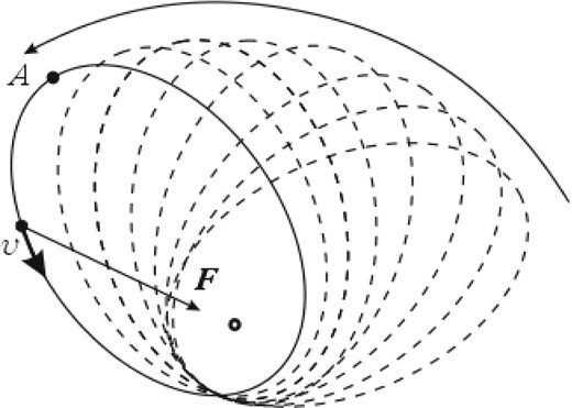
Apsidal precession of the Keplerian orbit.

Open in new tab Download slide

To test this approach, it is sufficient to believe that all stellar orbits in the ring with the boundaries R₂ > R₁ have the same semimajor axes and eccentricities:

\begin{equation} a = \frac{R_1 + R_2 }{2};\qquad e = \frac{R_2 - R_1 }{R_2 + R_1 }. \end{equation}

(14)

Then, equation (12) is

\begin{equation} \sigma (r) = \frac{M_r }{\pi ^2(R_1 + R_2)} \frac{1}{\sqrt{({R_2 - r})({r - R_1 })} }. \end{equation}

(15)

Let us introduce a mean density in the ring

\begin{equation} \bar{\sigma } = \frac{M_r }{\pi ({R_2^2 - R_1^2 })}, \end{equation}

(16)

Instead of equation (15), we have

\begin{equation} \sigma (r) = \frac{R_2 - R_1 }{\pi }\frac{\bar{\sigma }}{\sqrt{({R_2 - r})({r - R_1 })} }. \end{equation}

(17)

Because of the symmetry of the density law (17), the minimum is reached at the median circle r = a = (R₁ + R₂)/2 and is equal to

\begin{equation} \sigma _{\min } = \frac{2}{\pi }\bar{\sigma }. \end{equation}

(18)

Fig. 2 shows a typical density profile in the R-ring.

Figure 2.

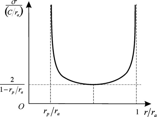
Typical surface density profile in the R-ring. The density has sharp lances at the edges and a deep internal minimum.

Open in new tab Download slide

The disc has a differential rotation. For example, we find the rotational energy of this disc to be

\begin{equation} T_{\rm rot} = \frac{1}{2}\int \!\!\!\int \limits _S {\sigma \upsilon _\theta ^2 {\rm d}S} = 2GM_r M_0 \frac{\sqrt{R_1 R_2 } }{(R_1 + R_2)^2}. \end{equation}

(19)

3 SPATIAL POTENTIAL OF THE R-RING

The spatial potential of the R-ring with the surface density law (17) was prepared in different forms (Kondratyev 1989, 2007). For the calculations, we apply the following formula:

\begin{equation} \varphi _{\rm d} ({r,x_3}) = \frac{2}{\pi ^2}\varphi _0 \int \limits _{ - ({\pi }/{2})}^{{\pi }/{2}} {\frac{z(\gamma )}{\sqrt{R^2 + x_3^2 } }} K(k)\,{\rm d}\gamma . \end{equation}

(20)

Here, φ₀ is the central annulus potential

\begin{equation} \varphi _0 = \varphi (0,0) = \frac{2M_{\rm d} G}{R_1 + R_2 } = \frac{M_{\rm d} G}{a} = 2\pi G\bar{\sigma }({R_2 - R_1}), \end{equation}

(21)

K(k) is the complete elliptic integral of the first kind and the module and auxiliary variables are

\begin{equation*} k = 2\sqrt{\frac{r \,z(\gamma )}{R^2 + x_3^2 }}, \end{equation*}

\begin{equation*} z(\gamma ) = \frac{R_2 - R_1 }{2}\sin \gamma + \frac{R_1 + R_2}{2}, \end{equation*}

\begin{equation} R({\gamma ,r}) = z(\gamma ) + r. \end{equation}

(22)

The potential in equation (20) is convenient because the integrated function disappears on the edges of the interval.

Calculations using equation (20) at x₃ = 0 are complicated because, for example, on the internal border, the module k → 1, and then the K(1) logarithmic disperses. These difficulties have been overcome in the following way. We kept the value (x₃/R₁), but considered it to be very small. In such a way, we calculated the surfaces of the identical potential in the space round the R-ring.

Fig. 3 shows the meridional lines of the equal potential of the R-ring. There is the separatrix, which is similar to a lemniscate. This separatrix separates two various families of equipotentials. The absolute maximum of the potential exists at an entrance to the ring in x₃ = 0, r = R₁. However, it is more convenient to study the potential of the R-ring in its main plane by using equation (26).

Lines of the equal potential for the R-ring. The potential normalized on (2/π2)φ0[1 − (R1/R2)]. The thick line shows the cross-section of the annulus. The relation of internal radius R1 to external radius R2 is 3: 5. We calculate 12 isolines (from external to internal), starting with 6.127125 up to 15.8855 with an interval of 0.887125 (Kondratyev 2007).

Figure 3.

Lines of the equal potential for the R-ring. The potential normalized on (2/π²)φ₀[1 − (R₁/R₂)]. The thick line shows the cross-section of the annulus. The relation of internal radius R₁ to external radius R₂ is 3: 5. We calculate 12 isolines (from external to internal), starting with 6.127125 up to 15.8855 with an interval of 0.887125 (Kondratyev 2007).

Open in new tab Download slide

4 ANNULUS POTENTIAL IN THE MAIN PLANE

We divide the wide ring into two parts: a ring with parameters R₁ ≤ x ≤ r, which is internal to the trial point r (where x is the intermediate radius), and the external ring to this point r with parameters r ≤ x ≤ R₂. The potential of the internal subsystem is denoted as φ₁(r), and the potential of the external subsystem is given by φ₂(r). Then, the potential of the whole ring to the point r is

\begin{equation} \varphi (r) = \varphi _1 (r) + \varphi _2 (r). \end{equation}

(23)

To find the components φ₁(r) and φ₂(r), we first note that the contribution to the potential at the point r from an elementary round hoop with the density μ = σ(r) dr is equal to

\begin{eqnarray} {\rm d}\varphi (r) &=& 4G\sigma (x) K \left( {\frac{r}{x}}\right)\,{\rm d}x,\qquad r \le x, \nonumber \\ {\rm d}\varphi (r) &=& \frac{4G}{r}x\sigma (x)K\left({\frac{x}{r}} \right)\,{\rm d}x,\qquad r \ge x. \end{eqnarray}

(24)

Integrating the contributions (24) on the respective intervals, we obtain the potentials of the first and second subsystems

\begin{eqnarray} \varphi _1 ( r ) &=& \frac{4G}{r}\int \limits _{R_1 }^r {x\sigma (x )K\left( {\frac{x}{r}} \right)\,{\rm d}x}, \nonumber \\ \varphi _2 ( r ) &=& 4G\int \limits _r^{R_2 } {\sigma ( x) K\left( {\frac{r}{x}} \right)\,{\rm d}x}. \end{eqnarray}

(25)

It should be noted that the modules in the complete elliptic integrals of the first kind in equation (25) are inverse to each other. Thus, in the main plane of the ring, we have the potential

\begin{eqnarray} \varphi _{\rm d} (r) &=& 4G\left[ {\frac{1}{r}\int \limits _{R_1 }^r {x\sigma ( x )K\left( {\frac{x}{r}} \right)\,{\rm d}x} + \int \limits _r^{R_2 } {\sigma (x)K \left( {\frac{r}{x}} \right)\,{\rm d}x} } \right]. \nonumber\\ \end{eqnarray}

(26)

In particular, in the centre of the R-ring, we again obtain equation (21).

Let us now introduce the normalized surface density |$\hat{\sigma }(r)$|

\begin{equation} \hat{\sigma }( r ) = \frac{\sigma ( r )}{\bar{\sigma }} = \frac{R_2 - R_1 }{\pi \sqrt{( {R_2 - r} )( {r - R_1 })} }, \end{equation}

(27)

and the normalized potential |$\hat{\varphi }( r )$|

\begin{eqnarray} \hat{\varphi }( r ) &=& \frac{\varphi _{\rm d} ( r )}{\varphi _0 }\nonumber\\ &=& \frac{2}{\pi ^2}\left[ {\frac{1}{r}\int \limits _{R_1 }^r\! {x\sigma ^{\circ }( x )K\left( {\frac{x}{r}} \right)\,{\rm d}x} + \int \limits _r^{R_2 } {\sigma ^{\circ }( x )K\left( {\frac{r}{x}} \right)\,{\rm d}x} } \right],\nonumber\\ \end{eqnarray}

(28)

where

\begin{equation} \sigma ^{\circ }( r ) = \frac{1}{\sqrt{( {R_2 - r})( {r - R_1 } )} }. \end{equation}

(29)

This potential has the absolute maximum at r = R₁,

\begin{equation} \varphi _{\max } = \frac{2\varphi _0 }{\pi ^2}\int \limits _{R_1 }^{R_2 } {\sigma ^{\circ }( x )K\left( {\frac{R_1 }{x}} \right)\,{\rm d}x}, \end{equation}

(30)

and the internal minimum, inside the ring on the outside border, at r = R₂,

\begin{equation} \varphi _{\min } = \frac{2\varphi _0 }{\pi ^2}\frac{1}{R_2 }\int \limits _{R_1 }^{R_2 } {x\sigma ^{\circ }( x )K\left( {\frac{x}{R_2 }} \right)\,{\rm d}x}. \end{equation}

(31)

It is also important to calculate the attraction force from the R-ring. For this purpose, it is necessary to find the derivative of the potential (28). After many transformations (see Appendix A), we obtain

\begin{eqnarray} r\frac{{\rm d}\varphi _{\rm d} }{{\rm d}r} &=& - \frac{2\varphi _0 }{\pi ^2} \Bigg \lbrace r\int \limits _{R_1 }^r {x\sigma ^{\circ }(x)\frac{E({{x}/{r}})}{r^2 - x^2}{\rm d}x}\nonumber \\ &&- \int \limits _r^{R_2 } {\sigma ^{\circ }(x) \left[ {\frac{x^2E({{r}/{x}})}{x^2 - r^2} - K\left( {\frac{r}{x}} \right)} \right]\,{\rm d}x} \Bigg \rbrace . \end{eqnarray}

(32)

Equation (32) works only at points outside the ring. At the borders and in the ring, the integrands in equation (32) have strong features that do not allow us to obtain the necessary numerical results. Therefore, we complement the calculations using equation (32) with calculations using equation (38).

5 EXAMPLES OF CALCULATING THE POTENTIAL IN THE MAIN PLANE

Using equation (28), we consider three variants of the R-ring:

a narrow ring with sizes R₁ = 0.5, R₂ = 0.6;
a ring with R₁ = 1, R₂ = 1.2 (Fig. 4 shows the normalized density as a function of x = r/R₁);
a wide ring with R₁ = 1, R₂ = 1.5.

Figure 4.

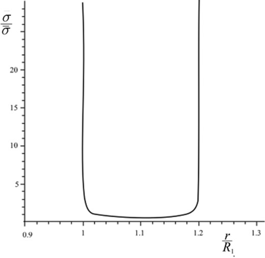
The surface density profile as a function of x = r/R₁. It is clearly visible that inside the ring, the profile is almost flat and the density depends weakly on the coordinates. Here, R₁ = 1 and R₂ = 1.2.

Open in new tab Download slide

For all three cases, Fig. 5 shows the distributions of the potential in the main plane. We show the general properties of such potentials. In the internal cavity of the R-ring (the interval from the centre to the inner edge R₁), the potential monotonically increases, and thus especially quickly in close proximity to the internal edge. At the points where there is a substance of the ring, the behaviour of the potential sharply changes and, little by little, it begins to decrease. After the external edge of the ring, the potential begins quickly to decrease. Such behaviour of the potential in the main plane of the ring agrees fully with the calculations of the 3D potential in Fig. 3. We see a similar behaviour of the potential in Section 8, where the calculation was carried out for the existing clockwise disc in the Milky Way.

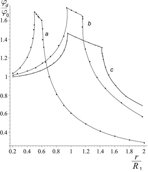
Distribution of the potential as a function of x = r/R1 for (a) R1 = 0.5, R2 = 0.6, (b) R1 = 1, R2 = 1.2 and (c) R1 = 1, R2 = 1.5. In the internal cavity of the R-ring (in the interval from the centre to the inner edge R1), the potential grows quickly enough. In the substance of the ring, the behaviour of the potential changes dramatically and it gradually begins to decrease. After the external edge of the ring, the potential begins quickly to decrease.

Figure 5.

Distribution of the potential as a function of x = r/R₁ for (a) R₁ = 0.5, R₂ = 0.6, (b) R₁ = 1, R₂ = 1.2 and (c) R₁ = 1, R₂ = 1.5. In the internal cavity of the R-ring (in the interval from the centre to the inner edge R₁), the potential grows quickly enough. In the substance of the ring, the behaviour of the potential changes dramatically and it gradually begins to decrease. After the external edge of the ring, the potential begins quickly to decrease.

Open in new tab Download slide

These calculations show that in the internal cavity of the R-ring (in the interval from the centre to the inner edge R₁), the potential monotonically increases. This leads to the fact that in this range the gas acts as the gravitational force, which is directed from the centre of the ring. If the R-ring is placed in the potential of the spherical (or spheroidal) bulge, the R-ring's own gravitational field leads to the local fall of the gas velocity rotation at r = R₁. Therefore, for a certain combination of parameters of the ring and bulge (or the black hole), the gravitational properties of the R-ring can become a physical cause, which explains the presence of additional local minima on the rotation curves of flat galaxies.

6 SUPERPOSITION OF THE GRAVITATIONAL FIELDS ‘R-RING + CENTRAL POINT MASS’ AND ‘R-RING + SPHERICAL BULGE’

First, we consider the addition of a potential of the central mass M₀ to the potential of the R-ring,

\begin{equation} \varphi _t = \frac{GM_0 }{r} + \varphi _{\rm d}, \end{equation}

(33)

where the potential of the ring is given by equation (28). Fig. 6 shows the total potential calculated on equation (33) for some combination of the parameters. It is important to note that there is a plateau on this curve at the boundary of the inner ring, which means that there is a reduction here in the velocity rotation of the gas.

Total potential ‘central point mass M0 + R-disc’ as a function of r/R1. For the calculations, we have taken the following model parameters: ring sizes R1 = 0.5 and R2 = 0.6 and the binding parameter (GM0/R1φ0) = 2.1. The influence of the R-ring is shown by the fact that near the inner boundary of the ring there is a narrow interval with a flattening (or plateau) of the potential graph, which means that there is a local decrease of the velocity rotation of gas.

Figure 6.

Total potential ‘central point mass M₀ + R-disc’ as a function of r/R₁. For the calculations, we have taken the following model parameters: ring sizes R₁ = 0.5 and R₂ = 0.6 and the binding parameter (GM₀/R₁φ₀) = 2.1. The influence of the R-ring is shown by the fact that near the inner boundary of the ring there is a narrow interval with a flattening (or plateau) of the potential graph, which means that there is a local decrease of the velocity rotation of gas.

Open in new tab Download slide

The mutual gravitational energy of the R-ring in the field of central mass M₀ is equal to

\begin{equation} W_{\rm m} = - \int \!\!\!\int \limits _S {\sigma (r)\varphi (r)\,{\rm d}S}. \end{equation}

(34)

Inserting σ(r) from equation (15), we have

\begin{equation} W_{\rm m} = - 2\frac{M_0 M_r G}{R_1 + R_2 }. \end{equation}

(35)

This energy is needed for the estimation of the disc stability.

We now take the inhomogeneous spherical bulge with such a density-potential pair:

\begin{eqnarray} \rho (r) &=& \rho _0 \left( {1 - \frac{r}{R}} \right); \nonumber \\ \varphi ^{\rm b}(r) &=& \frac{2}{3}\pi G\rho _0 \left( {R^2 - r^2 + \frac{r^3}{2R}} \right). \end{eqnarray}

(36)

Placing the R-disc in the given bulge, we find the full potential of such a system. It is important to emphasize that the internal potential of only one bulge everywhere monotonically decreasing also does not give any necessary effect. It is only with the advent of the R-ring that the situation changes. Fig. 7 shows that at the entrance to the ring, there is now also a plateau on the potential curve.

Total potential of the system ‘inhomogeneous spherical bulge +R-ring’ as a function of r/R1. For the calculations, we have taken the following model parameters: ring sizes R1 = 1 and R2 = 1.2 and the binding parameter (GM0/R1φ0) = 2.1. The plateau on this curve occurs when entering the ring inside.

Figure 7.

Total potential of the system ‘inhomogeneous spherical bulge +R-ring’ as a function of r/R₁. For the calculations, we have taken the following model parameters: ring sizes R₁ = 1 and R₂ = 1.2 and the binding parameter (GM₀/R₁φ₀) = 2.1. The plateau on this curve occurs when entering the ring inside.

Open in new tab Download slide

7 ROTATIONAL CURVES FOR THE CIRCULAR MOTION OF GAS IN THE GRAVITATIONAL FIELD ‘R-RING + BULGE’

As mentioned in the introduction, many rotation curves of flat galaxies have additional local minima. Fig. 8 shows a typical rotation curve with an additional local minimum.

Figure 8.

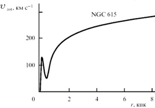
Rotation curve of the galaxy NGC 615 as a typical example of the profile velocity rotation of flat galaxies (Khoperskof & Friedman 2011).

Open in new tab Download slide

Such features on the rotation curves are successfully explained by the R-ring model.

For this purpose, we use the model of the inhomogeneous bulge (equation 36). The contribution to the square of the velocity rotation from the bulge is equal to

\begin{equation} r\frac{{\rm d}\varphi ^{\rm b}}{{\rm d}r} = - \frac{4}{3}\pi G\rho _0 r^2\left( {1 - \frac{3r}{4R}} \right). \end{equation}

(37)

The square of the total velocity is

\begin{eqnarray} \frac{V_{\rm rot}^2 }{\varphi _0 } &=& k_1 y^2\left( {1 - \frac{3R_1 }{4R}y} \right) + s_{1,2}, \nonumber \\ k_1 &=& \frac{4\pi G\rho _0 R_1^2 }{3\varphi _0 },\qquad y = \frac{r}{R_1 }. \end{eqnarray}

(38)

Here, s is a contribution from the R-ring. Because the gravitational force in the boundary points of the ring strives for infinity, inside and outside the ring we use the different functions s₁and s₂. So, out of the ring, we use the expression

\begin{eqnarray} &&\!\!\!s_1 = \frac{2}{\pi ^2}\Bigg \lbrace y\int \limits _1^y {\frac{xE({{x}/{y}})\,{\rm d}x}{({y^2 - x^2})\sqrt{[{({R_2}/{R_1 }) - x} ] ({x - 1})} }}\nonumber \\ &&\quad - \int \limits _y^{R_2 / R_1 } \frac{{\rm d}x}{\sqrt{[{({R_2 }/{R_1 }) - x} ] ({x - 1})} } \left[ {\frac{x^2E({{y}/{x}})}{x^2 - y^2} - K\left( {\frac{y}{x}} \right)} \right] \Bigg \rbrace . \nonumber\\ \end{eqnarray}

(39)

However, in the ring, it is better to use equation (20), which gives

\begin{equation} s_2 = - r \, \frac{\rm d}{{\rm d}r} \left( {\frac{\varphi _{\rm d} }{\varphi _0 }}\right), \end{equation}

(40)

where for calculations, it is necessary to take a sufficiently small value for x₃. Further transformations of equation (40) are given in Appendix B. The results of calculations by equations (37)– (40) are shown in Fig. 9.

Figure 9.

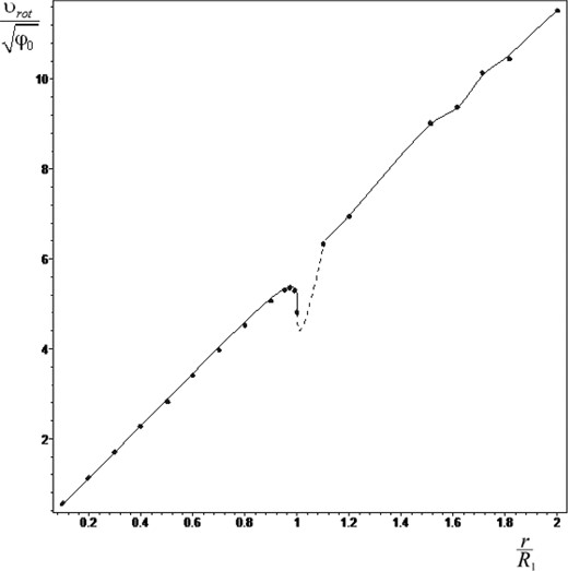
Rotation velocity profile in the potential ‘inhomogeneous spherical bulge + R-ring’ as a function of r/R₁. The parameters are R₁ = 1, R₂ = 1.5, x₃ = 0.001, R₁/R = 3 and k₁ = 33. The sharp local minimum appears at an entrance to the R-ring. There is also some evidence of a secondary minimum at an exit from the ring.

Open in new tab Download slide

By comparing Figs 8 and 9, we can see that observations are in good agreement with calculations for the R-ring model.

Thus, at an entrance to the R-ring, there is clearly a certain minimum of the velocity rotation.

In our model, it is now possible to make an assessment of the relation of the mass of the bulge to the mass of the ring. According to the second variant of equation (38) and equation (21) for the central potential, we find the coefficient

\begin{equation} k_1 = \frac{4\pi G\rho _0 R_1^2 }{3\varphi _0 } = 2\frac{M_{\rm b} }{M_r }\left( {\frac{R_1 }{R}} \right)^3\left( {1 + \frac{R_2 }{R_1 }} \right). \end{equation}

(41)

This allows us to make an assessment of the relation of masses M_b/M_r, which is necessary for the existence of a secondary minimum on the rotation curve. Thus, for the case

\begin{equation} R_1 = 1,\quad R_2 = 1.5,\quad \frac{R_1 }{R} = 3,\quad k_1 = 33, \end{equation}

(42)

we obtain from equation (41) the required mass ratio

\begin{equation} \frac{M_{\rm b} }{M_r } \approx 178. \end{equation}

(43)

The condition for the existence of the secondary minimum (more precisely, the lower limit for the mass ratio) is

\begin{equation} \frac{M_r }{M_{\rm b} } \ge 5 \times 10^{ - 3}. \end{equation}

(44)

8 APPLICATION TO THE CLOCKWISE DISC AND APSIDAL PRECESSION

Let us apply our model to numerical estimates for one particular example. In the Milky Way, a very compact cluster of B-stars with randomly oriented orbits is centred on the SMBH (Schödel, Merritt & Eckart 2009). Surrounding this compact cluster is a thin disc of younger stars, which is called the clockwise interval disc. We consider the clockwise coherently rotating stellar disc near the Galactic centre (Beloborodov et al. 2006; Lockmann & Baumgardt 2009). The geometrical sizes and mass of the disc are

\begin{eqnarray} R_1 &\approx & {1}\;{\rm arcsec}\; (0.04\, {\rm pc});\quad R_2 \approx 10 \;{\rm arcsec}\;(0.4\,{\rm pc});\nonumber \\ M_{\rm d} &\approx & 3 \times 10^5\,\mathrm{M}_ {{\odot }}. \end{eqnarray}

(45)

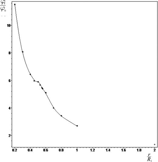
Here, we neglect the fact that the disc is blurred on the z-coordinate. We calculate the Newtonian potential in the main plane of the clockwise interval disc using equation (28). The results are shown in Fig. 10.

Dependence of the normalized potential for the clockwise stellar disc in the Milky Way as a function of r/R1. The parameters of the disc are given in equation (45). The vertical dotted lines mark the sizes of the disc. Calculations were carried out using equation (28).

Figure 10.

Dependence of the normalized potential for the clockwise stellar disc in the Milky Way as a function of r/R₁. The parameters of the disc are given in equation (45). The vertical dotted lines mark the sizes of the disc. Calculations were carried out using equation (28).

Open in new tab Download slide

The normalization figure was placed on the central potential φ₀, which, according to equation (21), is equal to

\begin{equation} \varphi _0 \approx 6 \times 10^{13}\;{\rm cm}^2\;{\rm s}^{ - 2}. \end{equation}

(46)

The cavity inside the ring is relatively narrow (0 < r ≤ 1 arcsec), but the inner edge is sharp, in agreement with the observations. The potential in the cavity monotonically increases. Then, with regards to the disc, the potential begins to decrease fluently, and the fall becomes steeper after the external edge of the disc.

The stars of the disc rotate round the SMBH with mass M_SMBH ≈ 4.4 × 10⁶ M_⊙ and the average value of the semimajor axis of the Keplerian orbits in the disc is equal to a₁ ≈ 5.5 arcsec (0.22 pc). According to equation (19), the rotational energy of the clockwise disc is

\begin{equation} T_{\rm rot} \approx 1.5 \times 10^{53}\,\mathrm{erg}. \end{equation}

(47)

For comparison, the mutual gravitational energy of the R-ring in the field of central mass M₀ in equation (35) is equal to

\begin{equation} W_{\rm m} \approx - 5.2 \times 10^{53}\,\mathrm{erg}. \end{equation}

(48)

Thus, the relation of the rotational energy to the module of mutual gravitational energy is very large and equal to

\begin{equation} \tau = \frac{T_{\rm rot} }{|{W_{\rm m} }|} \approx 0.29. \end{equation}

(49)

Consider now the case when the total potential is the sum of the potential of the R-disc and the potential of the point central mass M_SMBH. Instead of equation (33), we have

\begin{equation} \frac{\varphi _t }{\varphi _o } = \eta \frac{GM_{\rm SMBH} }{r} + \frac{\varphi _{\rm d} }{\varphi _o }, \end{equation}

(50)

where the binding parameter η of this model is very large,

\begin{equation} \eta = \frac{a}{R_1 }\frac{M_{\rm SMBH} }{M_{\rm d} } \approx 73. \end{equation}

(51)

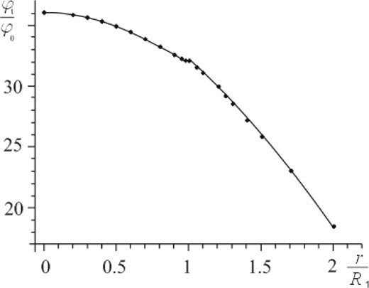
The potential of the clockwise disc in equation (50) is still given by equation (28). Fig. 11 shows the total potential calculated using equation (50). It is important to note that because the connective parameter (51) is large, the SMBH in the Milky Way suppresses the gravitation of the clockwise disc and the plateau of this curve is quite tiny (cf. Fig. 6).

Total potential ‘central point mass MSMBH + clockwise disc’ as a function of r/R1. The calculation was carried out using equation (50) with the real value of the connective parameter η = 73. The vertical dotted line marks a tiny plateau on this curve at the entrance to the ring.

Figure 11.

Total potential ‘central point mass M_SMBH + clockwise disc’ as a function of r/R₁. The calculation was carried out using equation (50) with the real value of the connective parameter η = 73. The vertical dotted line marks a tiny plateau on this curve at the entrance to the ring.

Open in new tab Download slide

Let discuss now an apsidal precession of the Keplerian orbits. There are two sources of this precession. The first source is the well-known relativistic effect for the precession of Keplerian orbit, of fixed a and e, in the field of the point mass M. For a black hole, the corresponding formula is

\begin{equation} \varepsilon _\bullet = 6\pi \frac{GM_{\rm BH} }{a({1 - e^2})c^2}. \end{equation}

(52)

This is the angular precession after one Kepler period. Then, the time of a complete turn of the apsidal line on 2π from the SMBH will be equal to

\begin{equation} T_{\rm prec} = N_\bullet T = 2\pi \frac{a^{{5}/{2}} ({1 - e^2})c^2}{3({GM_{\rm BH}})^{{3}/{2}}}. \end{equation}

(53)

Here,

\begin{equation} N_\bullet = \frac{a({1 - e^2})c^2}{3M_{\rm BH} G} = \frac{2c^2}{3GM_{\rm BH} }\frac{R_1 }{1 + n},\qquad n = \frac{R_1 }{R_2 } \end{equation}

(54)

is the number of turns of a body on an orbit.

For the SMBH in the Galaxy, we find the very large value T_prec ∼ 5 × 10⁸ yr, or N_• ∼ 10⁵. Even for stars with semimajor axes of the orbit a ≈ R₁, the time precession remains large, T_prec ∼ 7 × 10⁶ yr. Only for the star S2 nearest to the black hole (Gualandris, Gillessen & Merritt 2010) with semimajor axis a ≈ 0.119 arcsec and period equal to T_prec ≈ 26 593 yr, we do find N_• ∼ 1.75 × 10³.

However, there is also a second source of precession, which should be considered. This is because, in the central parsec of the Milky Way, in addition to the SMBH, there is a NSC of B-stars with mass M_* ∼ 10⁶ M_⊙ and the density distribution ρ ∼ c/r^1.8 (Schödel et al. 2009; Merritt 2013). This cluster of stars is the source of the mass precession, because of the distributed mass around the SMBH. There are two options.

In the first, we describe the mass precession, when the orbit of a trial star lies within the NSC. This case of an apsidal precession has been detailed and carefully considered by Merritt (2013). According to equation (4.88) of Merritt's book, the precession rate can be written in the following form:

\begin{equation} \frac{{\rm d}\omega }{{\rm d}t} = - \nu _r G_M ({e,\nu })\sqrt{1- e^2} \frac{M_ * (a)}{M_\bullet }, \end{equation}

(M55)

where ν_r = (2π)/T is the Kepler frequency, M_*(a) is the mass of the cluster within radius R = a, ν is an exponent in the density distribution ρ(r) ∼ c/r^ν (where ν ≈ 1.8 for the NSC) and G_M(e, ν) is the dimensionless function

\begin{equation} G_M ({e,\nu }) = - \frac{1}{2\pi e}\frac{3 - \nu }{2 - \nu }\int \limits _0^{2\pi } {{\rm d}x\cos x ({1 - e\cos x})^{2 - \nu }}. \end{equation}

(M56)

For example, for acceptable values for the clockwise disc, a₁ ≈ 5.5 arcsec (0.22 pc) and e ≈ 0.818, we have G_M(e, ν) ≈ 0.70954. By analogy with equation (54), let us now introduce the number N_* of turns of a star, required for a complete turn of the apsidal line on 2π because of precession from the NSC. Using equations (M55) and (52), we obtain the relation of time-scales:

\begin{eqnarray} \frac{N_\bullet }{N_ * } &=& \frac{|{\varepsilon ^ * }|}{\varepsilon _\bullet } = \frac{G_M ({e,\nu }) ({1- e^2})^{{3}/{2}}ac^2}{3GM_\bullet ^2 }M_ * (R),\quad \varepsilon _ * = \frac{{\rm d}\omega }{{\rm d}t}T. \nonumber\\ \end{eqnarray}

(57)

For the NSC in the Milky Way, equation (57) gives

\begin{equation} \frac{N_\bullet }{N_ * } = \frac{|{\varepsilon ^ * }|}{\varepsilon _\bullet } \approx 1.06 \times 10^4. \end{equation}

(58)

Thus, this mass precession is more important than the relativistic effect.

In the second case, we describe the apsidal precession of a trial star, when its orbit is outside the NSC. This can also take place and should be considered. However, unlike the case for internal orbits, it is now important to take into account the form of the cluster. To assess this case, we present the NSC inhomogeneous oblate spheroid with semiaxes a₁ ≥ a₃ and surfaces of equal density

\begin{equation} m = \frac{r^2}{a_1^2 } + \frac{x_3^2 }{a_3^2 },\qquad 0 \le m \le 1. \end{equation}

(59)

In agreement with observations, the density distribution in the NSC is ρ(m) = c/m^1.8 and the normalized second harmonic of the potential of this spheroid is equal to (Kondratyev 1989, 2007)

\begin{equation} J_2 = \frac{I_3 - I_1 }{M^ * a_1^2 } = \frac{e^{*2}}{3}\frac{\int _0^1 {m^4\rho (m)} \,{\rm d}m}{\int _0^1{m^2\rho (m)}\,{\rm d}m} = 0.125e^{ * 2}, \end{equation}

(60)

where |$e^{ * 2} = ({a_1^2 - a_3^2 })/{a_1^2}$| is the square of the eccentricity of the meridian section of the oblate spheroid. On the potential theory, the external potential of an axisymmetric body with precision up to the second-order harmonics (inclusive) is

\begin{equation} \varphi (r) = \frac{GM}{r}\left[ {1 - \frac{1}{2}J_2 \left( {\frac{a_1 }{r}} \right)^2 ({3\cos ^2\theta - 1})} \right], \end{equation}

(61)

where θ is the polar angle. The motion of a trial star in the equatorial plane of the body (θ = π/2) is under the influence of the potential of a point mass and J₂ is characterized by two frequencies (i.e. the average motion n and the radial frequency κ), which are approximately equal:

\begin{eqnarray} n = n_0 \sqrt{1 + \frac{3}{2}J_2 \left( {\frac{a_1 }{r}} \right)^2}, \nonumber \\ \nu = n_0 \sqrt{1 - \frac{3}{2}J_2 \left( {\frac{a_1 }{r}} \right)^2}. \end{eqnarray}

(62)

Here, n₀ = (2π)/T is the Kepler frequency, where n₀ ≡ ν_r in equation (M55). Then, the rate of an apsidal line is equal to

\begin{equation} \frac{{\rm d}\omega }{{\rm d}t} = n - \nu \approx \frac{3}{2}n_0 J_2 \left( {\frac{a_1 }{a}} \right)^2, \end{equation}

(63)

or the angular apsidal precession after one Kepler period is equal to

\begin{equation} \varepsilon ^ * = \frac{{\rm d}\omega }{{\rm d}t}T = 3\pi J_2 \left( {\frac{a_1 }{a}} \right)^2, \end{equation}

(64)

where a is the semimajor axis of the orbit of a test star. Given equations (52) and (64), we obtain the relations

\begin{equation} \frac{N_\bullet }{N_ * } = \frac{\varepsilon ^ * }{\varepsilon _\bullet } = \frac{1}{2}J_2 \frac{a(1 - e^2)c^2}{GM_{\rm BH} }\left({\frac{a_1 }{a}} \right)^2 \end{equation}

(65)

or

\begin{equation} \frac{N_\bullet }{N_ * } = \frac{\varepsilon ^ * }{\varepsilon _\bullet } = \frac{0.125e^{ * 2}}{2}J_2 \left( {\frac{a_1 }{a}} \right)^2\frac{a({1 - e^2})c^2}{GM_{\rm BH} }. \end{equation}

(66)

Substituting

\begin{equation*} M_{\rm SMBH} = 4.4 \times 10^6\,\mathrm{M}_{{\odot }},\qquad \frac{a_1 }{a} = 0.5,\qquad a = 0.6\,\mathrm{pc}, \end{equation*}

in order to assess the specific values, we obtain the relation of time-scales in the following form:

\begin{equation} \frac{N_\bullet }{N_ * } = \frac{\varepsilon ^ * }{\varepsilon _\bullet } \approx 4.4 \times 10^3 e^{ * 2}({1 - e^2}). \end{equation}

(67)

Fig. 12 shows the ratio of time-scales of the apsidal precession of Keplerian orbits in the clockwise disc according to equation (67).

Figure 12.

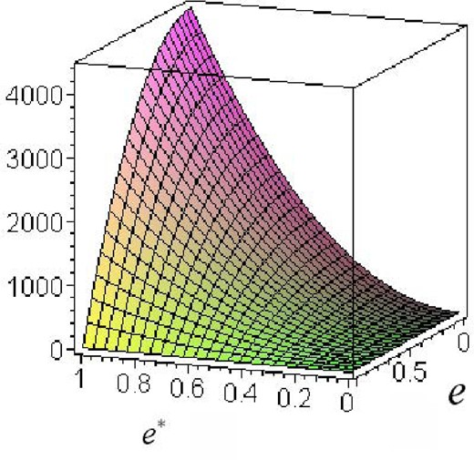
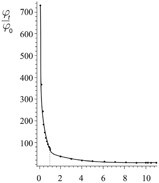
Ratio of time-scales of the apsidal precession of Keplerian orbits in the clockwise disc in the central parsec of the Milky Way. The second case is for an apsidal precession of a star, when its orbit is outside the NSC. Calculations were carried out using equation (67).

Open in new tab Download slide

For example, for the shape of the NSC with the value e* = 0.2 and the eccentricity of star orbit e = 0.5, according to equation (67) we obtain

\begin{equation} \frac{N_\bullet }{N_ * } = \frac{\varepsilon ^ * }{\varepsilon _\bullet } \approx 132. \end{equation}

(68)

From the physical point of view, the main features of the relation time-scales (67) are: (i) the strong dependence of the ratio on the shape of the cluster and from the value of eccentricity of the orbit of a trial star; (ii) the large value of the coefficient 4.4 × 10³. Acceptable values for the ratio of time-scales (67) are still quite large in favour of the second type of apsidal precession.

9 SUMMARY

We have considered the structure and 3D potential of the broad material ring (the R-ring), which consists of identical Kepler elliptic orbits, of fixed a and e, uniformly portioned on the azimuth angle. The density distribution in such rings is the result of 2D radially averaging of the mass of moving bodies. In principle, R-rings can also be filled with stellar orbits that precess around a star or black hole (rosette-like orbits). However, as calculations show, the time-scales associated with apsidal precession round a black hole for real stars in the clockwise disc are extremely large.

The potential of R-rings cannot be represented in analytical form. This circumstance complicates the calculation of the potential and the gravitational force of this ring. Therefore, it is necessary to unite various equations to calculate the potential of the R-ring. In particular, this allows us to calculate the spatial equipotential surfaces and to obtain the mutual gravitational energy of the R-ring in the field of the central mass M₀. The rotational energy of the stars of the ring was obtained, which is useful for investigating a stability configuration.

The R-rings can be formed in a natural way in dynamical systems with a large central mass. In galaxies, such R-rings are created by radially averaging the orbits of stars, which move around a massive black hole and in the NSC. Therefore, the use of R-ring models to study some questions in the dynamics of galaxies is quite justified. For example, in the framework of the model, we have calculated the ratio M_r/M_b ≥ 5 × 10⁻³, which is the lower limit for the existence of secondary maxima on the rotation curve. For the clockwise stellar disc in the Milky Way, we calculate its potential, the total potential of this disc in the field of the point central mass M_SMBH and the rotational energy of stars. For the relation of the rotational energy to the module of mutual gravitational energy, we find τ ≈ 0.29. The fact that this value τ exceeds the known criterion τ ≈ 0.14 (Ostriker & Peebles 1973) does not indicate the instability of this disc. In fact, the mass of the clockwise disc is known only very approximately and, besides, it is necessary to consider also the gravitational energy of the disc.

In spite of the huge mass of the black hole, the apsidal precession time of only one SMBH for stars in the real clockwise disc is extremely large. However, there is another source of apsidal precession, which is potentially even more important. This cluster of stars is the source of mass precession as a result of the distributed mass around the SMBH.

It is necessary to distinguish the apsidal precession for internal and external orbits. These two cases have different dynamic interpretations. For the case of inner orbits (Merritt 2013), the form of the cluster does not play a dominant role and a basic contribution to the effect brings in the spherical case. Taking into account the flattening of the cluster gives only small amendments to the main effect. In addition, the direction of motion of the apsidal line is the inverse. Because the relation of time-scales is equal to |ε*|/ε_• ≈ 10⁴, this mass precession is more important than the relativistic effect.

However, there is also a second case that describes the apsidal precession of trial stars, when their orbits are outside the NSC. For the case of external orbits, the form of the cluster plays an important role, because the rate of precession is proportional to the square of the eccentricity e*² of the meridian section of the oblate spheroid. In this case, the mass precession is more important than the relativistic effect. We note that the direction of rotation of the apsidal line here, as in the relativistic case, coincides with the direction of the orbital motion of the star.

It is also possible, apparently, that there is a mixed case, when the orbits of trial stars are partly beyond the boundary cluster.

Importantly, in both cases, the apsidal precession rate of trial stars in the central parsec in the Milky Way can largely be determined not to be a relativistic effect from the black hole, and the Newtonian gravitational influence of the densest stellar cluster around the SMBH.

In this paper we have considered the R-disc with one only set of a and e. The simple model provides an accurate calculation of some characteristics of real objects. However, in the future, we should create a superposition of R-discs. Such a complex disc created from elementary discs will have other profiles of density and potential and a wider range of applications.

I am very grateful to the referee for providing stimulating recommendations that have improved this work and to N. G. Trubitsyna for technical assistance.

REFERENCES

Antonov

V. A.

Nikiforov

I.

Kholshevnikov

K. V.

,

Elements of the Theory of the Gravitational Potential and Some Cases of its Explicit Expression

,

2008

Publishing House of St Petersburg State University

Google Scholar

Google Preview

OpenURL Placeholder Text

WorldCat

Beloborodov

A. M.

Levin

Y.

Eisenhauer

F.

Genzel

R.

Paumard

T.

Gillessen

S.

Ott

T.

,

ApJ

,

2006

, vol.

648

pg.

405

Crossref

Search ADS

Gualandris

A.

Gillessen

S.

Merritt

D.

,

MNRAS

,

2010

, vol.

409

pg.

1146

Crossref

Search ADS

Khoperskof

A. V.

Friedman

A. M.

,

Physics of Galactic Discs

,

2011

Moscow

Fizmatlit

Google Scholar

Google Preview

OpenURL Placeholder Text

WorldCat

Kondratyev

B. P.

,

Dynamics of Ellipsoidal Gravitating Figures

,

1989

Moscow

Nauka

Google Scholar

Google Preview

OpenURL Placeholder Text

WorldCat

Kondratyev

B. P.

,

The Potential Theory: New Methods and Problems with Solutions

,

2007

Moscow

Mir

Google Scholar

Google Preview

OpenURL Placeholder Text

WorldCat

Kondratyev

B. P.

,

Solar Syst. Res.

,

2012

, vol.

46

pg.

352

Crossref

Search ADS

Kondratyev

B. P.

Trubitsyna

N. G.

Mukhametshina

E. Sh.

Byrd

G. G.

et al. ,

ASP Conf. Ser. Vol. 316, Order and Chaos in Stellar and Planetary Systems

,

2004

San Francisco

Astron. Soc. Pac.

pg.

326

Google Scholar

Google Preview

OpenURL Placeholder Text

WorldCat

Lockmann

U.

Baumgardt

H.

,

MNRAS

,

2009

, vol.

394

pg.

1841

Crossref

Search ADS

Merritt

D.

,

Dynamics and Evolution of Galactic Nuclei

,

2013

Princeton, NJ

Princeton University Press

Google Scholar

Google Preview

OpenURL Placeholder Text

WorldCat

Ostriker

J. P.

Peebles

P. J. E.

,

ApJ

,

1973

, vol.

186

pg.

467

Crossref

Search ADS

Rubin

V. C.

Ford

W. K.

,

ApJ

,

1970

, vol.

159

pg.

379

Crossref

Search ADS

Schödel

R.

Merritt

D.

Eckart

A.

,

A&A

,

2009

, vol.

502

pg.

91

Crossref

Search ADS

Sofue

Y.

Rubin

V.

,

ARA&A

,

2001

, vol.

39

pg.

137

Crossref

Search ADS

Zacov

A. V.

Zotov

V. M.

,

Astron. Lett.

,

1989

, vol.

15

pg.

210

APPENDIX A: OBTAINING EQUATION (32)

Taking the derivative of equation (28), after some cuts we have

\begin{eqnarray} \frac{{\rm d}\varphi _{\rm d} (r)}{{\rm d}r} &=& \frac{2\varphi _0 }{\pi ^2}\Bigg [ - \frac{1}{r^2}\int \limits _{R_1 }^r {x\sigma ^{\circ }(x)K\left( {\frac{x}{r}} \right)\,{\rm d}x} \nonumber \\ &&+\, \frac{1}{r}\int \limits _{R_1 }^r {x\sigma ^{\circ }(x)\frac{\rm d}{{\rm d}r}K\left( {\frac{x}{r}} \right)\,{\rm d}x} \nonumber \\ && +\,\int \limits _r^{R_2 } {\sigma ^{\circ }(x)\frac{\rm d}{{\rm d}r}K\left( {\frac{r}{x}} \right)\,{\rm d}x} \Bigg ]. \end{eqnarray}

(A1)

Because

\begin{eqnarray} \frac{\rm d}{{\rm d}r} K\left(\frac{x}{r}\right) &=& \frac{K({{x}/{r}}) - [r^2E({{x}/{r}})/({r^2 -x^2})]}{r},\nonumber \\ \frac{\rm d}{{\rm d}r}K\left( {\frac{r}{x}} \right) &=& \frac{[{x^2E({{r}/{x}})}/({x^2 - r^2})] - K({{x}/{r}})}{r}, \end{eqnarray}

(A2)

after substituting equation (A2) into equation (A1) and making further reductions, we obtain the necessary equation (32).

APPENDIX B: TRANSFORMATION OF EQUATION (38)

Using equation (20), after a series of transformations we find

\begin{eqnarray} s_2 &=& \frac{4rz}{\pi ^2}\int \limits _{ -({\pi }/{2})}^{{\pi }/{2}} \Bigg \lbrace R \, K(k) - \left[ {\frac{E(k)}{1 - k^2} - K(k)} \right]\nonumber \\ &&\times\, \frac{({R^2 + x_3^2 - 2rR})\sqrt{R^2 + x_3^2 } }{4rz} \Bigg \rbrace \frac{{\rm d}\gamma }{({R^2 + x_3^2 })^{{3}/{2}}}. \end{eqnarray}

(B1)

For small values of x₃, this expression is used to calculate the velocity rotation.

Download all slides

Month:	Total Views:
March 2017	1
June 2017	1
September 2017	4
October 2017	7
December 2017	4
January 2018	2
February 2018	2
March 2018	11
April 2018	13
May 2018	13
June 2018	6
July 2018	13
August 2018	11
September 2018	10
October 2018	16
November 2018	11
December 2018	18
January 2019	16
February 2019	11
March 2019	15
April 2019	18
May 2019	23
June 2019	8
July 2019	14
August 2019	11
September 2019	7
October 2019	12
November 2019	12
December 2019	4
January 2020	13
February 2020	5
March 2020	3
April 2020	2
May 2020	4
June 2020	3
July 2020	6
August 2020	10
September 2020	6
October 2020	3
November 2020	5
December 2020	7
January 2021	5
February 2021	5
March 2021	15
April 2021	11
May 2021	4
June 2021	2
July 2021	6
August 2021	10
September 2021	17
October 2021	11
November 2021	7
December 2021	3
January 2022	8
February 2022	5
March 2022	10
April 2022	13
May 2022	1
June 2022	7
July 2022	7
August 2022	9
September 2022	13
October 2022	11
November 2022	11
December 2022	10
January 2023	7
February 2023	12
March 2023	7
April 2023	6
May 2023	7
June 2023	8
July 2023	13
August 2023	13
September 2023	8
October 2023	7
November 2023	4
December 2023	8
January 2024	3
February 2024	5
March 2024	3
April 2024	7
May 2024	10
June 2024	3
July 2024	4
August 2024	9
September 2024	2
October 2024	4
November 2024	5
December 2024	4
January 2025	5
February 2025	1
March 2025	17
April 2025	2
May 2025	6

Article Contents

Two-dimensional generalization of Gaussian rings and dynamics of the central regions of flat galaxies

Abstract

1 INTRODUCTION

2 STATEMENT OF THE PROBLEM

3 SPATIAL POTENTIAL OF THE R-RING

4 ANNULUS POTENTIAL IN THE MAIN PLANE

5 EXAMPLES OF CALCULATING THE POTENTIAL IN THE MAIN PLANE

6 SUPERPOSITION OF THE GRAVITATIONAL FIELDS ‘R-RING + CENTRAL POINT MASS’ AND ‘R-RING + SPHERICAL BULGE’

7 ROTATIONAL CURVES FOR THE CIRCULAR MOTION OF GAS IN THE GRAVITATIONAL FIELD ‘R-RING + BULGE’

8 APPLICATION TO THE CLOCKWISE DISC AND APSIDAL PRECESSION

9 SUMMARY

REFERENCES

APPENDIX A: OBTAINING EQUATION (32)

APPENDIX B: TRANSFORMATION OF EQUATION (38)

Citations

Views

Altmetric

Email alerts

Astrophysics Data System

Citing articles via

Latest

Most Read

Most Cited

Article Contents

Two-dimensional generalization of Gaussian rings and dynamics of the central regions of flat galaxies

Abstract

1 INTRODUCTION

2 STATEMENT OF THE PROBLEM

3 SPATIAL POTENTIAL OF THE R-RING

4 ANNULUS POTENTIAL IN THE MAIN PLANE

5 EXAMPLES OF CALCULATING THE POTENTIAL IN THE MAIN PLANE

6 SUPERPOSITION OF THE GRAVITATIONAL FIELDS ‘R-RING + CENTRAL POINT MASS’ AND ‘R-RING + SPHERICAL BULGE’

7 ROTATIONAL CURVES FOR THE CIRCULAR MOTION OF GAS IN THE GRAVITATIONAL FIELD ‘R-RING + BULGE’

8 APPLICATION TO THE CLOCKWISE DISC AND APSIDAL PRECESSION

9 SUMMARY

REFERENCES

APPENDIX A: OBTAINING EQUATION (32)

APPENDIX B: TRANSFORMATION OF EQUATION (38)

Citations

Views

Altmetric

Email alerts

Astrophysics Data System

Citing articles via

Latest

Most Read

Most Cited

This Feature Is Available To Subscribers Only