


Abstract
We introduce a new method for observationally estimating the fraction of momentum density (ρv) power contained in solenoidal modes (for which ∇ · ρv = 0) in molecular clouds. The method is successfully tested with numerical simulations of supersonic turbulence that produce the full range of possible solenoidal/compressible fractions. At present, the method assumes statistical isotropy, and does not account for anisotropies caused by (e.g.) magnetic fields. We also introduce a framework for statistically describing density–velocity correlations in turbulent clouds.
1 INTRODUCTION
As the principal sites of star formation in the local universe, molecular clouds demand much observational and theoretical attention. Their structure is extremely complex, driven by the interaction of supersonic turbulence, gravity, and magnetic fields (e.g. Elmegreen & Scalo 2004; Mac Low & Klessen 2004; McKee & Ostriker 2007; Chapman et al. 2011; Heyer & Brunt 2012). Theoretical descriptions of molecular clouds must begin with the structure of the relevant physical fields (density, velocity, etc.) in three dimensions (3D), while our practical information is necessarily restricted to what can be measured from the projection of these fields on to the observational axes – two spatial and, for spectral line data, one (line-of-sight) velocity component. It is a crucially important, yet challenging, problem to relate the projected fields to intrinsic properties of the 3D physical fields.
Only limited information about the 3D density field, ρ(x, y, z), can be derived via analysis of the projected 2D column density field, N(x, y), which is observationally obtained by extinction measurements, dust emission, or integrated spectral line intensities. For the latter, we may be aided by (or perhaps limited by) density-selectivity of particular molecular transitions, yet molecular line emission is the only source of information for studying the dynamics of molecular clouds.
Arguably the most useful property of N(x, y) is that its Fourier transform, |$\tilde{N}(k_{x}, k_{y})$|, is directly proportional to a 2D slice through the Fourier transform of the density field, |$\tilde{\rho }(k_{x}, k_{y}, k_{z})$|, where the line-of-sight wavevector, kz = 0; i.e. |$\tilde{N}(k_{x}, k_{y}) \propto \tilde{\rho }(k_{x}, k_{y}, k_{z} = 0)$|. This allows, under the assumption of isotropy, the density power spectrum to be derived (e.g. Stutzki et al. 1998), the 3D density variance to be inferred (Fischera & Dopita 2004; Brunt, Federrath & Price 2010a, hereafter BFP), and an estimate of the 3D density probability distribution function (PDF) to be constructed (Brunt, Federrath & Price 2010b). The essence of the BFP method (relating the 2D normalized column density variance to the 3D normalized density variance) lies in determining the fraction of variance contained in a single 2D slice of the 3D power spectrum.
While BFP focused primarily on a method to relate density and column density statistics, they also presented a brief outline of the same method applied to velocity fields, though noting that the natural observational density-weighting of the velocity field would potentially cause problems. In this paper, we present an extended development of the outline method presented in BFP, subject to two key modifications. First, the density-weighting of the velocity field means that the physical field suitable for BFP-like analysis is the ‘momentum density’ field, |${\rho }{\boldsymbol {v}}$|, rather than the velocity field alone. Secondly, the realization that only transverse (solenoidal) modes (for which |$\nabla \cdot {\rho }{\boldsymbol {v}} = 0$|) are projected into 2D allows us to extend the BFP method to estimate the fraction of momentum density power that is held in solenoidal modes, if given an estimate of the total momentum density power (through a spectral line imaging observation). The ideas underpinning the extended method are presented below, along with a demonstration of its applicability using numerical simulations of turbulent clouds. The method as presented assumes statistical isotropy, so should not be applied to clouds for which significant anisotropy is observed or suspected due to (e.g.) the presence of a strong magnetic field at low Mach numbers (BFP).
The layout of this paper is as follows. In Section 2, we present the method for observationally estimating the fraction of momentum power in transverse modes, after first introducing the background considerations necessary for its formulation. In Section 3, we describe the numerical simulations to be used for testing purposes. In Section 4, we test the method by applying it to the numerical simulations, followed by a discussion (Section 5) and summary (Section 6). In the appendix, we examine statistical aspects of density–velocity correlation, which has a small effect on the method.
2 SOLENOIDAL AND COMPRESSIBLE MODES
In this section, we discuss geometrical properties of divergence-free (‘transverse’ or ‘solenoidal’) and curl-free (‘longitudinal’ or ‘compressible’) modes in a general vector field (Section 2.1), before considering the consequences of projection of such a field from 3D to 2D (Section 2.2). In the following, we will use transverse/solenoidal and longitudinal/compressible to refer, respectively, to divergence-free and curl-free components. Subsequently, we identify the momentum field as the most relevant physical field of interest for quantitative analysis and develop a method by which the fraction of power in transverse momentum modes may be estimated observationally (Section 2.3).
2.1 General considerations
The Helmholtz Decomposition (equation 1) is unique, up to a vector constant, provided that the field |$\boldsymbol {F}$| falls to zero on its outer boundary. More generally, |$\boldsymbol {F}$| could in principle contain a contribution from a curl-free, divergence-free component, |$\boldsymbol {F}_{L}$|, given by the gradient of a scalar harmonic field ϕL that satisfies the Laplace equation (∇2ϕL = 0). Specifically, the curl-free nature of |$\boldsymbol {F}_{L}$| follows from its definition as the gradient of a scalar, while its divergence-free nature requires that ϕL satisfies the Laplace equation. As a harmonic field, ϕL must obey the mean value theorem, i.e. that its value at any point |${\boldsymbol {x}}$| is equal to its average on any spherical surface of arbitrary radius surrounding |${\boldsymbol {x}}$|. This means that ϕL can contain no local maxima or minima, and therefore that any maxima/minima must occur on its outer boundary. The properties of ϕL are therefore determined entirely by boundary conditions: |$\boldsymbol {F}_{L} = {\nabla }\phi _{L}$| will quantify large-scale, smooth gradients in |$\boldsymbol {F}$| that cannot be assigned to either |${\boldsymbol {F}}_{\perp }$| or |${\boldsymbol {F}}_{||}$|.
For our study here, we use numerically simulated fields (with the momentum density |${\rho }{\boldsymbol {v}}$| playing the role of |$\boldsymbol {F}$|) that obey periodic boundary conditions. For these fields, the multiplicity of choices for the ‘boundary’ and the condition of no local maxima/minima ensure that ϕL is a constant and therefore that |$\boldsymbol {F}_{L} = 0$|, and the Helmholtz Decomposition is unique. For real momentum fields encountered in the interstellar medium (ISM), we must rely on finding clouds that are sufficiently isolated that boundary conditions on |${\rho }{\boldsymbol {v}}$| are not a concern. Our method is therefore best-suited to molecular clouds that are bounded in space (i.e. by a fall-off in density ρ that ensures no non-zero |${\rho }{\boldsymbol {v}}$| values on their boundary).
The more widely distributed atomic medium is less suited to application of our method, since it will be difficult to ensure the absence of large-scale gradients in any finite field. Finally, it should be noted that |${\rho }{\boldsymbol {v}}$| will be continuous across the atomic/molecular transition and restriction to the molecular component is a necessarily limited description of the ISM as a single fluid – not to mention restriction to practically observable regions using trace molecules, and the possible influence of inter-mixed atomic/molecular zones. However, these problems are not in principle insurmountable (with sufficient data) though they may pose considerable challenges if a complete description of the ISM fluid is desired.
2.2 Projection from 3D to 2D
Consider the case where we have access to only one scalar component of the vector field |${\boldsymbol {F}}$|. We assume that the accessible component is oriented along the line of sight (as in, for example, a spectral line observation), which we take as the z-direction. The observable component of |${\boldsymbol {F}}$| is then Fz = Fz⊥ + Fz|| where Fz⊥ and Fz|| are the z components of the transverse and longitudinal parts of |${\boldsymbol {F}}$|. The contribution of Fz to the Fourier-transformed field – |$\tilde{\boldsymbol {F}}(\boldsymbol {k})$| – is |$\tilde{F}_{z}$| and this is oriented along the kz-direction (i.e. |$F_{z} \hat{\boldsymbol {z}}$| transforms into |$\tilde{F}_{z} \hat{\boldsymbol {k}}_{z}$| where |$\hat{\boldsymbol {z}}$| and |$\hat{\boldsymbol {k}}_{z}$| are unit vectors in the z and kz directions, respectively).
The condition |$\boldsymbol {k} \cdot \tilde{\boldsymbol {F}}_{\perp } = 0$| requires that |$\tilde{F}_{z\perp } = 0$| along the kz axis (where kx = ky = 0). Clearly we must also find that |$\tilde{F}_{z\perp } = \tilde{F}_{z}$| everywhere in the plane kz = 0, since there the condition |$\boldsymbol {k} \times \tilde{\boldsymbol {F}}_{||} = 0$| requires that |$\tilde{F}_{z||} = 0$| in this plane.
To illustrate the above power spectra, we show example 3D renderings of |$\tilde{F}_{z\perp } \tilde{F}_{z\perp }^{*}$| and |$\tilde{F}_{z_{||}} \tilde{F}_{z_{||}}^{*}$| in Fig. 1. Isotropic power spectra of |$\tilde{{\boldsymbol {F}}}_{\perp } \cdot \tilde{{\boldsymbol {F}}}_{\perp }^{*} \propto k^{-4}$|, and |$\tilde{{\boldsymbol {F}}}_{||} \cdot \tilde{{\boldsymbol {F}}}_{||}^{*} \propto k^{-4}$| have been assumed. The power spectrum of the longitudinal component of Fz has a characteristic ‘hourglass’ appearance, resulting from the suppression (nulling) of power near (at) kz = 0. Since |${\tilde{\boldsymbol {F}}}_{||}$| is aligned with |${\boldsymbol {k}}$|, this means that |$\tilde{F}_{z_{||}}$| must be zero in the kz = 0 plane. Conversely, the transverse power is maximized (at fixed k) in the plane kz = 0, and diminishes as |kz/k| approaches unity. An instructive reference point can be obtained by considering the power distributions along the line (kx = 0, ky = 0, kz ≠ 0). Here, the longitudinal power is entirely contained in the z-component, while the transverse power is equally split (assuming isotropy) between the x-component and the y-component (equations 17 and 19 with kx = ky = 0).
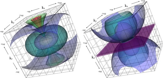
3D renderings of constant power surfaces in the power spectra of Fz⊥ (left) and |$F_{z_{||}}$| (right), given by equations (15) and (14), respectively. Isotropic power spectra: |$\tilde{{\boldsymbol {F}}}_{\perp } \cdot \tilde{{\boldsymbol {F}}}_{\perp }^{*} \propto k^{-4}$|, and |$\tilde{{\boldsymbol {F}}}_{||} \cdot \tilde{{\boldsymbol {F}}}_{||}^{*} \propto k^{-4}$| have been assumed. In both panels, the origin of coordinates (|$\boldsymbol {k} = 0$|) lies in the centre of the image.
2.3 Observational considerations
We now review the information provided by spectral line observations of the ISM, with a view to determining which physical field(s) may be analysed by the above system. The principal requirements for such a field are (1) that it is a 3D vector field, and (2) that one of its components can be projected (or averaged) over the line of sight with no weighting by other variable physical fields. It turns out, as explained below, that the momentum density field, |${\boldsymbol {p}} = \rho {\boldsymbol {v}}$|, (hereafter simply ‘momentum’) most closely satisfies these requirements. Application of the method to velocity fields is impossible except under conditions of uniform density, which are essentially never encountered in the ISM. Below we therefore develop a scheme whereby the fraction of momentum power in transverse modes may be estimated observationally – i.e. evaluation of equation (31).
At this point, we identify the following ratio: |$\sigma ^{2}_{p_{z,p}}/\sigma ^{2}_{p_{z}}$| – i.e. the fraction of z-momentum power (variance) projected into 2D – as the most relevant quantity to estimate observationally, since measurements of |$\sigma ^{2}_{p_{z,p}}/\sigma ^{2}_{p_{z}}$| and f⊥(k) are needed for the evaluation of equation (31). We already have f⊥(k), as this can be derived from the angular average of the power spectrum of W1(x, y) (note that the overall normalization is unimportant).
Above, we have computed |$\langle \rho v^{2}_{z} \rangle /\langle \rho \rangle$| via the observable ratio W2/W0, but note that it may also be computed simply as the dispersion of the summed spectral line profile of the data. It is also important to recognize that a finite-width thermal/instrumental broadening term will cause overestimation of |$\langle \rho v^{2}_{z} \rangle /\langle \rho \rangle$|. The simple fix for this is to subtract the thermal/instrumental dispersion from the raw measurement of |$\langle \rho v^{2}_{z} \rangle /\langle \rho \rangle$| (i.e. the influence of finite thermal/instrumental broadening is simply to convolve the δ-function-mapped data with a smoothing kernel on the vz-axis which will be typically Gaussian in form). We will return to this point, and other practical observational considerations in Section 4 below.
2.4 Summary of observational measurements required
Finally, we note that in equation (55), it is evident that some factors cancel, suggesting further simplification is possible. We have opted to leave it in the form presented since we believe it makes more logical sense this way, and the individual terms (in square brackets) in the equation will be analysed below, along with the deprojection factor, B, in Section 4.
3 NUMERICAL SIMULATIONS
The simulations used to test the analytic method were performed with the astrophysical code flash (Fryxell et al. 2000; Dubey et el. 2008), which integrates the ideal, 3D, magnetohydrodynamic (MHD) equations of compressible gas. The MHD equations were closed with a polytropic equation of state, |$P_\rm{th}=c_\rm{s}^2\rho$|, such that the gas remains isothermal with a constant sound speed, cs. We solve the MHD equations in the hydrodynamic limit (|${\boldsymbol {B}} = 0$|) on 3D, uniform grids with a fixed resolution of 2563 grid points and periodic boundary conditions, using a positive-definite Riemann solver for ideal MHD (Waagan, Federrath & Klingenberg 2011).
Starting from a uniform density distribution and zero velocities, the forcing excites turbulent motions, which approach a statistically steady state after about two turbulent crossing times, |$2T=L/(\mathcal {M}c_\rm{s})$| (e.g. Klessen, Heitsch & Mac Low 2000; Klessen 2001; Heitsch, Mac Low & Klessen 2001; Federrath, Klessen & Schmidt 2009; Federrath et al. 2010; Price & Federrath 2010; Micic et al. 2012; Federrath 2013), where |$\mathcal {M}$| denotes the 3D, root-mean-squared sonic Mach number. We study simulations in both the subsonic and supersonic regimes of turbulence with |$\mathcal {M}\sim 0.1$|, 0.5, 2, 5 and 15, each with the two limiting cases of purely solenoidal and purely compressive forcing to basically cover the whole range of possible solenoidal momentum ratios between zero and unity, in order to test the analytic method. To ensure that the initial transient phase (t ≲ 2T) is not included in the following analysis, we consider snapshots at t = 3, 4 and 5 T. Each of the snapshots used in the analysis is thus separated by at least one crossing time, effectively representing statistically independent turbulent fields at this temporal separation. We thus improve the independent statistical sampling of our results by including these three snapshots for each simulation, providing an estimate of the typical temporal variations of our results.
We also make use of previously conducted simulations for auxiliary information and testing purposes. These simulations have been previously described in BFP and comprise smoothed particle hydrodynamics (SPH) simulations of solenoidally forced turbulence at a range of (supersonic) Mach numbers and fixed grid simulations of solenoidally forced MHD turbulence at a range of (supersonic) Mach numbers and a range of magnetic field strengths (see BFP for more details).
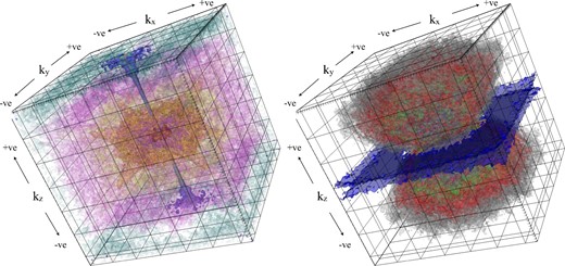
3D renderings of constant power surfaces in the power spectra of pz⊥ (left) and |$p_{z_{||}}$| (right) in a snapshot taken from the numerical simulations (solenoidally forced, rms Mach number = 5). In both panels, the origin of coordinates (|$\boldsymbol {k} = 0$|) lies in the centre of the image (cf. Fig. 1).
4 APPLICATION TO HYDRODYNAMIC SIMULATIONS
We now apply the above method to the numerical simulations described in Section 3. Before doing so, we examine the fraction of momentum power contained in transverse modes by direct calculation in 3D. These fractions are calculated via Fourier space, making use of the conditions given in equations (5) and (6). In Fig. 3, we plot the ratio of transverse to total momentum power, |$\sigma ^{2}_{p_{\perp }} / \sigma ^{2}_{p}$|, against the density-weighted Mach number, |${\mathcal {M}_{1}}$|. At low Mach number (|${\mathcal {M}_{1}} <\!{<} 1$|), the different forcing methods result in very different values of |$\sigma ^{2}_{p_{\perp }} / \sigma ^{2}_{p}$| – essentially all the power remains in the respective forcing modes. As |${\mathcal {M}_{1}}$| increases, the transverse fractions appear to converge to |$\sigma ^{2}_{p_{\perp }} / \sigma ^{2}_{p} \approx 0.7\pm 0.1$|, irrespective of the nature of the forcing. It is perhaps unfortunate that this situation arises; interestingly, the transverse velocity power fraction is different for different forcing mechanisms, even at high Mach number (Federrath et al. 2011). We discuss the prospects of measuring the transverse velocity power fraction below.
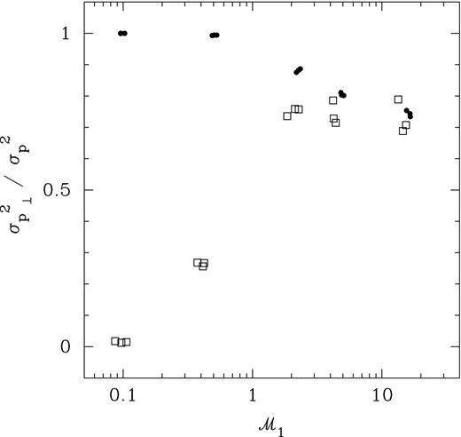
Plot of the fraction of momentum power in transverse modes versus 3D density-weighted Mach number, |${\mathcal {M}}_{1}$|. Dots: solenoidal forcing; open squares: compressive forcing.
Now we attempt to measure |$\sigma ^{2}_{p_{\perp }} / \sigma ^{2}_{p}$| using only observationally accessible quantities. The analysis below is somewhat idealized, in that we assume certain auxiliary pieces of physical information are available, and we do not consider the effects of instrumental noise and beam smearing – though we will make comments and recommendations at appropriate points.
4.1 Normalized density variance
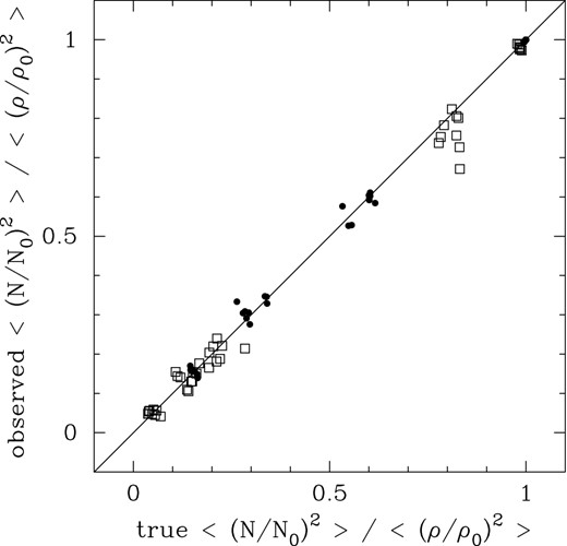
Observed versus intrinsic values of the ratio 〈(N/N0)2〉/〈(ρ/ρ0)2〉 measured in the numerical simulations. The ‘observed’ values are calculated using the BFP method, which is accurate to about 10 per cent for statistically isotropic fields.
4.2 Dispersion in z-axis momentum
The next term in equation (52) we examine is the third term, |$g_{21} \langle \rho v_{z}^{2} \rangle / \langle \rho \rangle$|. This term is designed to measure the total dispersion in z-axis momentum (divided by 〈ρ2〉) as described by equation (50) – or equivalently, the z-axis velocity dispersion calculated with a ρ2 weight. As mentioned previously, 〈ρv2〉/〈ρ〉 can either be obtained from the ratio 〈W2〉/〈W0〉 or by the dispersion of the summed spectral line profile. The latter option is probably best-suited to practical observational work, though the two are equivalent. Corrections for thermal/instrumental broadening should be made. We point out here that for the low Mach number simulations (|${\mathcal {M}} {<} 1$|), the thermal broadening dominates over the turbulent motions of interest. Here, we assume no thermal broadening (or exact accounting for it) which is rather unrealistic. However, our aim here is to test the principle rather than the practice, since the low Mach number simulations extend the range of |$\sigma ^{2}_{p_{\perp }} / \sigma ^{2}_{p}$| available for analysis (see Fig. 3). We do not recommend that the method is applied practically to subsonic media, but expect instead that it will be applied to large molecular clouds where the thermal broadening has a small influence on the dominant supersonic turbulent motions.
A further idealization that we use here is that we work with Mach numbers rather than velocity dispersions. This is just a convenient system in which to make comparisons between velocity dispersions (in units of the squared sound speed), though we note that our estimation of the parameter ϵ needed to derive g21 via equation (A16) requires the Mach number |${\mathcal {M}}_{1}$| to be known. In the observational context, this would require that an accurate measure of the sound speed is available. We have made a further assumption here, which is: the use of equation (A16) assumes the hydrodynamic limit, since the fit was made to simulations that did not include magnetic fields. There is an apparent dependence of ϵ on the Alfvénic Mach number (see Fig. A4) but this is only important in the limit |${\mathcal {M}}_{\rm A} {<} 1$| and low sonic Mach number (|${\mathcal {M}}_{1} \lesssim 5$|). We assume that auxiliary observations have been made to ensure that these conditions are not met, though the consequences of erroneously assuming they are not met when in fact they (at least within the range of conditions covered by the above analysis) are not severe. In the low |${\mathcal {M}}_{\rm A}$|, low |${\mathcal {M}}_{1}$| regime, ϵ is slightly smaller than that which holds in the hydrodynamic limit (ϵ∞), and therefore the true correction factor lies between unity and g21(ϵ∞). As shown below, the practical difference between these two cases is tolerably small.
From the simulation data, we can directly extract the quantity |${\mathcal {M}}_{1z} = \langle \rho v^{2}_{z} \rangle / \langle \rho \rangle c^{2}_{\rm s}$|, which is the ρ-weighted z-velocity dispersion in units of the squared sound speed. The correction factor g21 is designed to convert this into the ρ2-weighted z-axis Mach number: |${\mathcal {M}}_{2z} = \langle \rho ^{2} v^{2}_{z} \rangle / \langle \rho ^{2} \rangle c^{2}_{\rm s}$|. To calculate ϵ we assume isotropy and take |${\mathcal {M}}_{1} = \sqrt{3} {\mathcal {M}}_{1z}$|, allowing us to calculate g21 = 〈(ρ/ρ0)2〉−ϵ using equation (A15) with 〈(ρ/ρ0)2〉 already calculated above. In Fig. 5(a), we plot |$M^{2}_{1z}$| versus |$M^{2}_{2z}$| (measured with privileged access) for the supersonic data, to illustrate the consequences of the naive assumption that |$M^{2}_{1z}$| is a good surrogate for |$M^{2}_{2z}$|. Fig. 5(b) shows the effect of assuming that |$M^{2}_{2z} = g_{21} M^{2}_{1z}$|, which is rather better, though there are a couple of outliers that resist correction (these are notably anisotropic fields). In Fig. 5, we have again used all 3 available choices for the z-axis in each simulation. In the analysis below, we will document the effect of including or ignoring the correction factor g21.
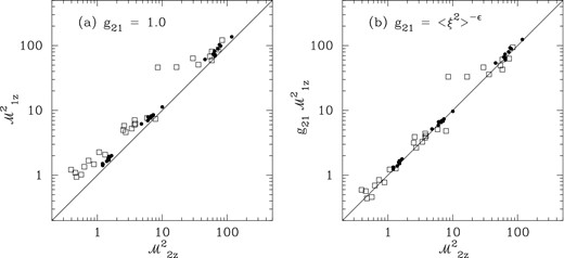
(a) Estimate of |${\mathcal {M}}_{2z}^{2}$| naively assuming |${\mathcal {M}}_{2z}^{2} = {\mathcal {M}}_{1z}^{2}$|; (b) estimate of |${\mathcal {M}}_{2z}^{2}$| assuming |${\mathcal {M}}_{2z}^{2} = g_{21} {\mathcal {M}}_{1z}^{2}$|.
4.3 Projected solenoidal fractions
The first factor in equation (52) is trivially computed using the observationally accessible |$\langle W^{2}_{1} \rangle / \langle W^{2}_{0} \rangle$|. We have already mentioned accounting for the contribution of noise variance to |$\langle W^{2}_{0} \rangle$|, and it remains to deal with the role of noise in calculating |$\langle W^{2}_{1} \rangle$|, which is a bit more complicated. We just mention here that prescriptions for accounting for noise in centroid velocity measurements are available (e.g. Kleiner & Dickman 1985; Miesch & Bally 1994; Brunt & Mac Low 2004) and a suitable modification of these should be made.
Now with all three terms in equation (52) assembled, we can construct an observationally accessible estimate of |$\sigma ^{2}_{p_{z,p}} / \sigma ^{2}_{p_{z}}$| (i.e. the fraction of z-momentum power projected into 2D) for comparison with the same ‘true’ quantity directly extracted from the data with privileged access. Fig. 6 shows this comparison, (a) without and (b) with the correction factor g21 applied. In general, equation (52) provides an accurate observational measure of the ratio |$\sigma ^{2}_{p_{z,p}} / \sigma ^{2}_{p_{z}}$|.
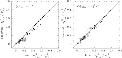
Observationally estimated values of the fraction of total z-momentum power projected into 2D assuming (a) g21 = 1 (i.e. no statistical correction for density–velocity correlation) and (b) g21 = 〈ξ2〉−ϵ, in both cases plotted versus the true value of this fraction.
Note that there are two main effects that control this ratio. First, if the fraction of compressive (longitudinal) momentum modes is high, then the ratio |$\sigma ^{2}_{p_{z,p}} / \sigma ^{2}_{p_{z}}$| will be low since only transverse modes are projected into 2D. This is (partially) why the compressively forced simulations display small values of |$\sigma ^{2}_{p_{z,p}} / \sigma ^{2}_{p_{z}}$|. Secondly, a higher density variance will typically result in a lower fraction of momentum variance projected into 2D since such fields suffer more averaging/smoothing of small-scale structure (e.g. as mentioned above in the discussion of Fig. 4). This means that even though the transverse momentum fractions are approximately the same at high Mach numbers regardless of the forcing mechanism (see Fig. 3) the compressive forcing drives higher density variance (Federrath, Klessen & Schmidt 2008) which results in a greater degree of line-of-sight averaging of small-scale structure, and therefore lower values of |$\sigma ^{2}_{p_{z,p}} / \sigma ^{2}_{p_{z}}$|. The highest values of |$\sigma ^{2}_{p_{z,p}} / \sigma ^{2}_{p_{z}}$| reached (∼1/3) originate from the subsonic solenoidally forced simulations which have very nearly uniform density. In this case, trivially, ∼1/3 of the momentum variance is projected along one of the three spatial axes.
4.4 Deprojection
The final step in the analysis is the de-projection via equation (53) to estimate the fraction of momentum power in transverse modes in 3D (assuming that |$\sigma ^{2}_{p_{\perp }} / \sigma ^{2}_{p} \approx \sigma ^{2}_{p_{z\perp }} / \sigma ^{2}_{p_{z}}$|). The input to the de-projection factor is just f⊥(k), obtained from the angular average of the power spectrum of W1. In an observational context, this should be corrected for noise (using a suitable modification of the methods in Brunt 2010; Brunt & Mac Low 2004) and treatment of the effect of the telescope beam pattern should be included (see BFP for a discussion of this).
In Fig. 7, we compare the observationally derived values of |$\sigma ^{2}_{p_{\perp }} / \sigma ^{2}_{p}$| to those measured exactly with privileged access to the momentum field in 3D. Fig. 7(a) shows the comparison with no statistical correction for density–velocity correlation, while Fig. 7(b) shows the results with the g21 correction applied (we have applied the correction to all data, not just the supersonic fields). In the plots, the plotted points are the mean values of |$\sigma ^{2}_{p_{\perp }} / \sigma ^{2}_{p}$| obtained by averaging the results over all three spatial axes, while the error bars represent the standard deviation about the mean. This is to show the recovery of |$\sigma ^{2}_{p_{\perp }} / \sigma ^{2}_{p}$| from the same field seen from different orientations. Overall, the observational recovery of the intrinsic |$\sigma ^{2}_{p_{\perp }} / \sigma ^{2}_{p}$| values is good, albeit with relatively large scatter for the high Mach number compressively forced simulations.

Observationally estimated values of the fraction of 3D momentum power in transverse modes assuming (a) g21 = 1 (i.e. no statistical correction for density–velocity correlation) and (b) g21 = 〈ξ2〉−ϵ, in both cases plotted versus the true value of this fraction.
Though the solenoidally forced simulations alone span a limited range in |$\sigma ^{2}_{p_{\perp }} / \sigma ^{2}_{p}$|, the recovery is reliable, albeit with a slight overestimation for intrinsic |$\sigma ^{2}_{p_{\perp }} / \sigma ^{2}_{p} \approx 1$| (applicable to the subsonic, ∼ uniform density fields). If the turbulence was strongly magnetized (i.e. |$\mathcal {M}_{\rm s} \lesssim 5$|, |$\mathcal {M}_{\rm A} \lesssim 1$|), but assumed not to be, then the g21 factors derived from ϵ∞ would lead to slightly overestimated solenoidal fractions, though for the range of Mach numbers studied here, this is only at the ∼10 per cent level. This should be tested directly in future studies, where the (probably) more important question of anisotropy should be assessed.
5 DISCUSSION
While the simulated fields here contain a number of idealizations (Fourier-space driving, periodic boundary conditions, lack of self-gravity, strict isothermality) the above analysis has demonstrated that, in principle, the fraction of momentum power in transverse (solenoidal) modes, |$\sigma ^{2}_{p_{\perp }} / \sigma ^{2}_{p}$|, may be measurable from observations. (We have outlined practical observational considerations at appropriate points above.) For the subsonic fields, to extend the range of intrinsic |$\sigma ^{2}_{p_{\perp }} / \sigma ^{2}_{p}$| available, we have assumed (unrealistically) that the dominant thermal broadening terms have been accounted for.
We envision that the above method is best-suited to the study of nearby supersonically turbulent molecular clouds for which high-sensitivity, high spatial dynamic range spectral line data are available. So, how relevant are the simulated supersonic fields to typical conditions met in molecular clouds that (currently) could be analysed with the above model? We argue that the key condition that must be satisfied is that of statistical isotropy, rather than any shortcomings in the physical simulations – i.e. the simulations simply create an intrinsic ratio |$\sigma ^{2}_{p_{\perp }} / \sigma ^{2}_{p}$| that we can set out to measure. If strong magnetic fields are present, then this could cause significant anisotropy in the density and velocity fields that we have not accounted for here. The assumption of isothermality may be slightly problematic, since the method relies (weakly) on applying corrections for thermal broadening and deriving the Mach number (to estimate g21). The assumption of a single Mach number is also problematic if the method is to be applied to the atomic ISM. It is also possible of course that the detailed physics may affect the statistical correction factors g21, a point to which we will return below.
5.1 Anisotropies and discontinuities
The next steps in the testing of the method should focus on possible complications and biases induced by anisotropies. In fact, there are suggestions that compressive modes may be suppressed in highly anisotropic media (Hansen, McKee & Klein 2011), which would be very interesting to test observationally once the practicalities of doing so are understood more fully. Testing (or extension) of the method to MHD case with different compressive/solenoidal fractions is also worth pursuing. Filamentary structure, by itself, poses no particular problem as long as the filament orientations are statistically isotropic. In practice, good evidence for isotropy in projected 2D is needed, as well as some confirmation that the cloud's line-of-sight depth is comparable to its projected extent. In the field selection, one must also pay attention to the boundary conditions. In our simulations, these are periodic, so there are no problems arising from edge discontinuities. Fields for analysis should be selected so that no significant edge discontinuities exist, though we are aided in this selection by the ρ- (or N-) weighting of the relevant fields so that (to the extent that any ‘cloud’ is truly isolated) a suitable region may be defined where W0, W1 and W2 are sufficiently close to zero that this condition is satisfied. Edge-tapering (e.g. Brunt & Mac Low 2004) or padding (e.g. Brunt 2010) may be applied to sufficiently large fields, with negligible quantitative consequences.
5.2 Variability
In terms of the reliability of the recovered |$\sigma ^{2}_{p_{\perp }} / \sigma ^{2}_{p}$|, of most concern is the relatively high degree of scatter in the compressively forced fields. The scatter is mainly a consequence of the high degree of variability in these fields, so that variances are contributed to strongly by a small number of extreme field values, perhaps magnifying any anisotropic effects. To quantify this, in Fig. 8 we plot the root-mean-square uncertainty on the measured |$\sigma ^{2}_{p_{\perp }} / \sigma ^{2}_{p}$| ratios against a measure of the column density variability, |$\ln {\left(1 + \sigma ^{2}_{N/N_{0}}\right)}$| (which would be the logarithmic variance, |$\sigma _{ln(N/N_{0})}$|, in the case of a lognormal PDF). Fig. 8 shows that typical errors are at the ∼10 per cent level or better for |$\ln {\left(1 + \sigma ^{2}_{N/N_{0}}\right)} \lesssim 1$|, but then increase sharply for |$\ln {\left(1 + \sigma ^{2}_{N/N_{0}}\right)} \gtrsim 1$|.
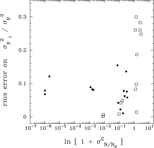
The root-mean-square uncertainty on the measured |$\sigma ^{2}_{p_{\perp }} / \sigma ^{2}_{p}$| ratios from Fig. 7, plotted against a measure of the column density variability, |$\ln {(1 + \sigma ^{2}_{N/N_{0}})}$|.
5.3 Variations in solenoidal/compressive fractions
It is evident from Fig. 3 that the |$\sigma ^{2}_{p_{\perp }} / \sigma ^{2}_{p}$| ratio does not allow observational discrimination between solenoidal and compressive forcing, since the |$\sigma ^{2}_{p_{\perp }} / \sigma ^{2}_{p}$| ratios appear to converge to 0.7 ± 0.1 at high Mach numbers independent of the nature of the forcing (it is probably unlikely that these curves cross, though we cannot say more at present). However, given that observational estimates of |$\sigma ^{2}_{p_{\perp }} / \sigma ^{2}_{p}$| have not yet been made, it would be an interesting and important test to see if this ratio (∼0.7 ± 0.1) is realized in nature and whether there may be systematic variations in different environments. Note that, though mathematically well defined, the forcing scheme is somewhat idealized physically – assigning accelerations in Fourier space, which generate non-local accelerations in direct space. It is possible that the |$\sigma ^{2}_{p_{\perp }} / \sigma ^{2}_{p}$| ratios seen here may not necessarily be replicated in real molecular clouds, where large-scale driving sources could include supernovae or spiral shocks.
One could also consider the initially point-like energy injections from outflows in localized regions generating different |$\sigma ^{2}_{p_{\perp }} / \sigma ^{2}_{p}$| ratios. It may also be possible that |$\sigma ^{2}_{p_{\perp }} / \sigma ^{2}_{p}$| could evolve with time in decaying conditions (our simulations here are continually driven) or due to an increasing importance of self-gravity over time. Observational application of this method therefore may be more revealing and interesting than simply confirming the ‘default’ ∼0.7 ± 0.1 ratio seen in the current simulations. A framework for investigating the respective roles of solenoidal and compressive forcing in determining the normalized density variance has been recently presented by Konstandin et al. (2012b), and it would be interesting to compare (or combine) that method with ours.
The inclusion of self-gravity will be particularly interesting. Federrath et al. (2011) have shown that gravitational collapse produces a high fraction of longitudinal modes, which are later converted to solenoidal modes. It may therefore be possible to search for this signature in molecular clouds, after we have validated the method for the self-gravitating case. This is beyond the scope of the current work, but we note that the geometrical constraints, that lead to projection of solenoidal modes only, will not be affected by inclusion of self-gravity. It is true, however, that self-gravity will have a notable effect on the density PDF, and presumably on the degree of density–velocity correlation. A number of theoretical studies have looked at the generation of ∼power-law tails in density PDFs (e.g. Klessen 2000; Kritsuk, Norman & Wagner 2011; Federrath & Klessen 2013; Girichidis et al. 2014) and corresponding features have been seen observationally: early-time PDFs appear ∼lognormal in form, while more evolved clouds have more prevalent power-law tails in their density PDFs (e.g. Kainulainen et al. 2009; Schneider et al. 2013, 2014; Kainulainen, Federrath & Henning 2014).
5.4 Improvements
In the further testing of this model (in addition to the key question of anisotropy), there are two main areas that should be investigated. First, in terms of numerics, we need more information on the role of density–velocity correlations (Section 4) by measuring ϵ over a greater range of physical conditions, including the effects of self-gravity, as mentioned above, and a more detailed investigation of magnetic fields. In the analysis completed above, we have introduced the concept of ϵ and the correction factors gmn and demonstrated their use in practice. Admittedly, there was a degree of internal ‘tuning’ of ϵ employed, though we did support the measured ϵ values with independent data, and the correction terms g21 here are close enough to unity to be of not overwhelming concern. More important, perhaps, is the possible role that the statistical system presented in Section 4 may play in other contexts for understanding density–velocity correlations in turbulent media.
The second main avenue for improvement will be in the investigation of more mundane observational considerations, such as excitation and opacity. The analysis presented above was completed under the assumption of uniform excitation and in the optically thin limit, and therefore serves as a baseline for quantifying how variable excitation and finite opacity affect the method. Naively, this would make the measurements of |$\sigma ^{2}_{p_{\perp }} / \sigma ^{2}_{p}$| less reliable, and possibly biased, but may also have the advantageous effect of taming some of the field variability.
5.5 Other moments
Finally, we have based the method around the recovery of the fraction of momentum power, 〈ρ2v2〉, in transverse modes simply because the momentum field satisfies the observational requirement that it is projected into 2D unweighted by any other physical fields. One could also consider the fraction of velocity dispersion, 〈v2〉, in transverse modes (which is sensitive to the forcing mechanism – Federrath et al. 2011) or indeed the fraction of energy, 〈(1/2)ρv2〉, in transverse modes – either of which, arguably, more naturally spring to mind as relevant quantities to measure. The prospects for measuring either of the two above-named alternatives to momentum power are rather dim however, since neither field is accessible as a projected quantity observationally (except in the case of uniform density when all three definitions are equivalent).
In the general case where the density is variable, neither the velocity nor energy can be isolated for independent study. For example, note that the z-component of the momentum field, which is projected unweighted into 2D, is the product of the density, ρ, and z-velocity, vz. Therefore, the crucially important (projected) power spectrum of W1 involves the 3D convolution of the Fourier transforms of ρ and vz, of which a single plane (kz = 0) is available for analysis. To isolate the velocity contribution, one could in principle imagine deconvolving the density contribution for a simply structured density field (e.g. a 3D Gaussian or spatial power law), but for the highly complex and variable density fields encountered in the ISM, this appears futile. One possible way to proceed is to form an understanding of the relation between the three quantities (〈v2〉, 〈(1/2)ρv2〉, and 〈ρ2v2〉) by a means similar to the statistical system presented in the appendix – because the different quantities are just different ρq-weighted velocity dispersions. The stumbling block is simply that the Fourier space power distributions may be rather different, so that the deprojection factors become unreliable. In this case, an understanding of any scale-dependence of the statistical relationship between 〈v2〉, 〈(1/2)ρv2〉, and 〈ρ2v2〉 would be required, as well as an understanding of their transverse/longitudinal mode dependence. These considerations are beyond the scope of the current paper, but may be a worthwhile pursuit in future studies.
6 SUMMARY
In this paper, we have introduced an observational method for measuring the fraction of momentum power in solenoidal modes in a turbulent cloud, and confirmed its applicability using hydrodynamic numerical simulations. The method is best-suited to application in nearby molecular clouds for which high-sensitivity, high spatial dynamic range spectral line observations are available. The principal limitation of the method at present is its reliance on the assumption of isotropy. Further work is needed to examine the impact of anisotropy imposed by (e.g.) magnetic fields (BFP) or anisotropic driving of turbulence (Hansen et al. 2011). Isotropy aside, the main limiting factor in the accuracy of the model is variability in the physical fields (density, momentum). We have also introduced a statistical framework for describing density–velocity correlations in turbulent media that should be of relevance beyond its application here.
A big thanks to Daniel Price for allowing us use of the auxiliary numerical simulations, to Maria Cunningham for allowing us access to the Delta Quadrant Survey data and to Dave Acreman for much-needed help with Figs 1 and 2. CB is funded in part by the UK Science and Technology Facilities Council grant ST/J001627/1 (‘From Molecular Clouds to Exoplanets’) and the ERC grant ERC-2011-StG_20101014 (‘LOCALSTAR’), both held at the University of Exeter. CF acknowledges funding provided by the Australian Research Council under the Discovery Projects scheme (grant DP110102191). Supercomputing time at the Leibniz Rechenzentrum (project pr32lo) and at the Forschungszentrum Jülich (project hhd20) are gratefully acknowledged. The software used in this work was in part developed by the DOE-supported ASC/Alliance Center for Astrophysical Thermonuclear Flashes at the University of Chicago.
REFERENCES
APPENDIX A: DENSITY–VELOCITY CORRELATIONS
In Section 2.3, we introduced a correction factor g21, needed to convert a ρ-weighted velocity dispersion into a ρ2-weighted velocity dispersion. Here, we discuss the procedural steps necessary to evaluate the relationship between |$\langle \rho v^{2}_{z} \rangle /\langle \rho \rangle$| and |$\langle \rho ^{2} v^{2}_{z} \rangle /\langle \rho ^{2} \rangle$|, in order to derive the statistical correction factor g21 introduced in Section 2.3.
As we demonstrate below, if the density and velocity field are statistically uncorrelated (i.e. they have independent probability distributions), then |$\langle \rho v^{2}_{z} \rangle /\langle \rho \rangle = \langle \rho ^{2} v^{2}_{z} \rangle /\langle \rho ^{2} \rangle$|, and therefore g21 = 1. In general, this will not be the case, so in the following we introduce and test a simple method for quantifying the degree of density–velocity correlation and establish a simple prescription for converting between different ρq-weighted velocity dispersions. After theoretical development (Sections A1 and A2) and testing (Section A3), we examine existing observational constraints on these corrections (Section A4).
A1 Theoretical development
A2 Formulation for lognormal density PDFs
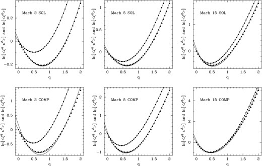
The spectrum of moments for 〈ξq〉 (dots) and 〈ξqv2〉 (triangles) versus q. The curve (described in the text) is fitted to 〈ξq〉 and shifted to best match 〈ξqv2〉 in order to determine ϵ.
A3 Numerical testing
The applicability of equation (A9) to the numerical density and velocity fields can be tested by calculating and comparing 〈ξqv2〉(q) and 〈ξq〉(q). From the simulated data, moments between q = 0 and q = 2 in steps of 0.05 were calculated in the zero momentum frame, using the full 3D velocity field. To ensure that the resulting values of ϵ are not simply ‘tuned’ to the numerical simulations analysed in this paper, we use a much larger sample of density and velocity fields by including the simulations from BFP. These include both hydrodynamic simulations (using SPH) and MHD simulations (using grid calculations) – see Section 3 and BFP for more details. We only consider supersonic fields in this analysis, since the influence of density fluctuations in subsonic fields is minimal – we will return to this point at the end of this section.
After calculation of the moments, a sixth-order polynomial in q (|$\sum _{n=0}^{6} c_{n} q^{n}$|) was fitted to ln (〈ξq〉). Following this, the same polynomial with the same (fixed) cn was fitted to ln (〈ξqv2〉) with additional offset (ϵ) and scaling factor (A) – i.e. |$\ln (A) + \sum _{n=0}^{6} c_{n} (q - \epsilon )^{n}$|.
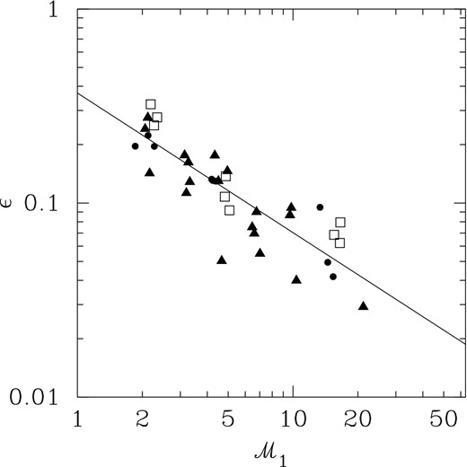
Plot of ϵ versus 3D density-weighted Mach number, |${\mathcal {M}}_{1}$|, derived from the hydrodynamic grid simulations (dots: solenoidal forcing; open squares: compressive forcing; triangles: hydrodynamic (SPH) simulations with solenoidal forcing from BFP.
The values of ϵ obtained from the MHD simulations are shown in Fig. A3, where they are plotted versus |${\mathcal {M}}_{1}$|. Relative to the hydrodynamic results, represented by the straight line (ϵ∞), the MHD fields tend to give lower values of ϵ at the lower Mach numbers. We find that in the low |${\mathcal {M}_{1}}$| regime, ϵ appears to decrease with decreasing Alfvénic Mach Number, |${\mathcal {M}}_{\rm A}$|, as shown in Fig. A4, where we have plotted ϵ/ϵ∞ versus |${\mathcal {M}}_{\rm A}$|. However, an |${\mathcal {M}}_{\rm A}$|-dependence (if any) is less clear at higher |${\mathcal {M}}_{1}$|. In the analysis below, we will adopt ϵ∞, obtained in the hydrodynamic limit, as the basis for deriving correction factors (g21).
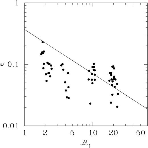
Plot of ϵ versus 3D density-weighted Mach number, |${\mathcal {M}}_{1}$|, derived from the MHD simulations (BFP). For reference, we have shown the fitted line from Fig. A2.
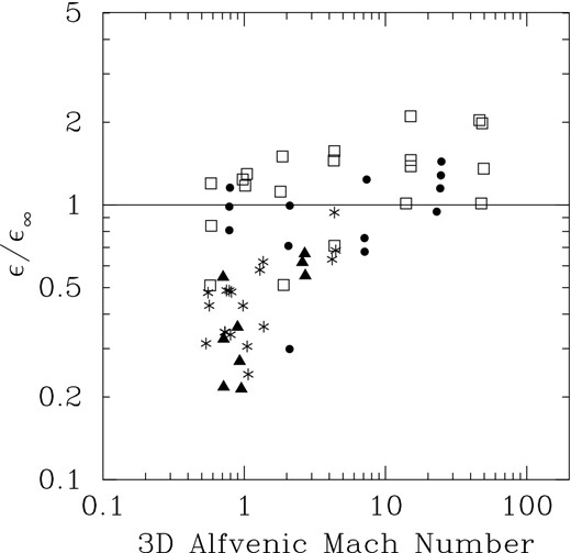
Plot of ϵ (relative to the fitted |$\epsilon _{\infty }({\mathcal {M}}_{1})$| relation in the hydrodynamic limit) versus 3D Alfvénic Mach number. Symbols denote the rms sonic Mach number in the simulation (open squares: |${\mathcal {M}}_{1} = 20$|; dots: |${\mathcal {M}}_{1} = 10$|; triangles: |${\mathcal {M}}_{1} = 4$|; asterisks: |${\mathcal {M}}_{1} = 2$|).
For a given 〈ξ2〉, a smaller ϵ leads to a correction factor (g21) closer to unity. In fact, at fixed sonic Mach number, numerical simulations suggest that 〈ξ2〉 should be closer to unity for strongly magnetized turbulence than for hydrodynamic turbulence (Molina et al. 2012). Together with lower ϵ, this would predict that g21 should be closer to unity for strongly magnetized turbulence than for the hydrodynamic case.
Finally, as mentioned previously, we have only considered supersonic fields in the above analysis. Since the velocity dispersion ratios (equation A14) depend on 〈ξq〉 to the power −(m − n)ϵ, fields for which 〈ξq〉 ≈ 1 (i.e. uniform or weakly varying density fields) require large values of ϵ for small corrections. We find that measurement of ϵ in this regime (by the method given above) is rather unstable, with ϵ increasing strongly, with large scatter, as |$\langle \xi ^{q} \rangle \longrightarrow 1$|. In the analysis in Section 4, we will nevertheless investigate values of the correction factor g21 extrapolated into the subsonic regime.
A4 Constraints from observational data
In the preceding analysis, we made the assumption that the velocity dispersion decreases with the density at which it is measured (i.e. equations A4 and A5), and explored the consequences on velocity dispersions calculated with a ρq-weight. To do this, privileged access to the density and velocity fields in 3D is required, so this is not possible to do observationally by exactly the same method. An alternative means of constraining the effect of such density–velocity correlations is to interpret equations (A4) and (A5) literally and examine velocity dispersions measured observationally in different density regimes.
A4.1 Constraints from Larson's relations
The Larson (1981) relations between velocity dispersion (or linewidth) and cloud size (σv ∝ La) and between density and cloud size (ρ ∝ L−b) can provide a very crude measure of ϵ in molecular clouds. Combining the two relations gives a measure of ϵ ≈ a/b, though with some major caveats. The original a = 0.38 and b = 1.1 derived by Larson (1981) give ϵ = 0.35, while values of a ≈ 0.5 and b = 1 (assuming Virial equilibrium) give ϵ ≈ 0.5 from Solomon et al. (1987). Large-scale CO surveys use size, linewidth and mean density measured in distinct clouds rather than probing the density-dependence of velocity dispersion internal to individual clouds. Extending such cloud/clump-based analyses to ‘subcloud’ scales are highly questionable (e.g. Ballesteros-Paredes & Mac Low 2002; Schneider & Brooks 2004), but nevertheless tend to yield values of a and b roughly in accord with the large-scale values, though in the presence of significant scatter. Using the analysis of Simon et al. (2001) on four inner Galaxy clouds (in the Solomon et al. 1987 survey region), we find values of ϵ between 0.17 and 0.39 (the lower values being mostly due to shallower linewidth–size relations than that found by Solomon et al. 1987).
Criticisms have been levelled at the density-size relation as being a consequence of limited dynamic range in cloud surface density (e.g. Vázquez-Semadeni, Ballesteros-Paredes & Rodriguez 1997). Using the Solomon et al. (1987) cloud sample, Heyer et al. (2009) found that, over the limited surface density range available, velocity dispersions rose with surface density as σv ∝ Σ1/2 at fixed cloud size. If we make the reasonable assumption that higher surface density indicates higher volume density, then a/b should provide an upper limit to ϵ.
The ϵ values derived here by Larson's relations are quoted for reference, and should be compared to the better-motivated (and notably lower) values derived below, using density-selective tracers.
A4.2 Constraints from density-selective tracers
A4.3 Observational estimates of ϵ
In this section, we will estimate a few contrasting values of ϵ from observational data.
McQuinn et al. (2002) examined CS (J = 2–1) and 13CO (J = 1–0) emission in the inner Galaxy observed as part of the Galactic Ring Survey (Jackson et al. 2006) and found no significant difference between CS (J = 2–1) and 13CO (J = 1–0) velocity dispersions, as evidenced by roughly constant brightness temperature ratios for composite spectra averaged over large clouds (many parsec scale). The critical densities of CS (J = 2–1) and 13CO (J = 1–0) are ∼103 cm−3 and ∼5 × 105 cm−3 respectively. Equation (A18) in this case finds ϵ is ‘very small’ (the g21 correction factor in our lognormal model above would therefore simply be ∼ unity – i.e. no correction). However, McQuinn et al. (2002) ultimately concluded that subthermal excitation was a probable factor in the line excitation (especially for CS) so that the effective critical densities would be lower than nominal.
To examine this more closely, we have used multitracer spectral line data, spanning a larger range in critical density, from the Delta Quadrant Survey (see Lo et al. 2009). Fig. A5 shows three regions within the survey where spectral lines are single-component and allow easy fitting of Gaussian functions to estimate their dispersions. We have averaged the intensities over the boxes shown and determined velocity dispersions for each of the four transitions (C18O 1–0, CS 2–1, HCO+ 1–0 and HNC 1–0). The spectra, with fitted Gaussians, are also shown in Fig. A5, along with the variation of velocity dispersion with critical density of the tracer. From this, we determine ϵ ≈ 0.
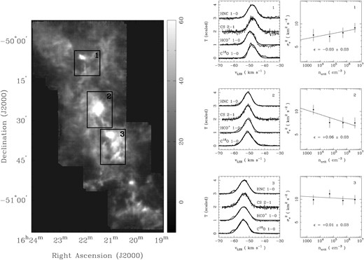
Three subregions in the Delta Quadrant Survey, in which the intensities of C18O 1–0, CS 2–1, HCO+ 1–0, and HNC 1–0 spectral lines have been averaged and fitted with Gaussians to determine their velocity dispersions – shown in the centre panel, with spectra scaled to their peak and offset for clarity. In the right-hand panel, we plot log velocity dispersion versus log critical density to determine ϵ as the slope of a fitted line for each region.
Williams & Blitz (1998) examined CS (J = 2–1) and 13CO (J = 1–0) and (J = 3–2) emission from a star-forming cloud (the Rosette nebula) and a non-star-forming cloud (G216, ‘Maddalena's Cloud’). They found small differences in clump internal velocity dispersion in the (J = 3–2) and (J = 1–0) 13CO lines: slightly broader 3–2 lines in the Rosette, relative to 1–0 (implying ϵ < 0 in this case, since the critical density of the 3–2 line is ∼10 times that of the 1–0 line); slightly narrower lines are found for 3–2 in G216, relative to 1–0. They attribute this behaviour to local feedback effects close to star-forming sources in the Rosette, which have no counterparts in the less active G216. Williams & Blitz (1998) do not report values for the linewidth ratios, but they can be estimated from their fig. 19; we will take |$\sigma ^{2}_{v,3-2}/\sigma ^{2}_{v,1-0}$| ≈ 2 and |$\sigma ^{2}_{v,3-2}/\sigma ^{2}_{v,1-0}$| ≈ 0.5 as representative for the Rosette and G216, respectively. These lead, assuming nc, 3−2/nc, 1−0 ≈ 10, to ϵRosette ≈ −0.3 and ϵG216 ≈ +0.3. These values of ϵ are notably larger in magnitude than those found for our numerical simulations (and in the case of the Rosette involve a sign change) but may not be representative values for globally determined ϵ as we require. A negative value of ϵ probably cannot be maintained over all densities (over all space), though one could potentially imagine high-density clumps moving through a relatively static low-density substrate as a possible configuration for this. The negative value of ϵ for the Rosette more likely comes instead from (e.g.) outflows injecting energy locally in a characteristic density regime near the J=3–2 critical density. Such behaviour could cause problems for our simple power law characterization in equation (A5).
McQuinn et al. (2002) made large-scale averages of line profiles to produce their CS–13CO comparisons, which is more closely matched to our requirements. In contrast, Williams & Blitz (1998) examined linewidths from targeted clumps, where the role of density–velocity correlations are likely to be most emphasized. With this provison in mind, we now examine the CS/13CO (J = 1–0) velocity dispersion ratios found by Williams & Blitz (1998). These are |$\sigma ^{2}_{v,{\rm{CS}}}/\sigma ^{2}_{v,{\rm{13CO}}}$| ∼ 0.7 (Rosette) and |$\sigma ^{2}_{v,{\rm{CS}}}/\sigma ^{2}_{v,{\rm{13CO}}}$| ∼ 0.5 (G216). Taking a critical density ratio of 500, we then find ϵRosette ≈ +0.06 and ϵG216 ≈ +0.11. With a larger baseline in critical density (and comparable hν/k values for the transitions), these CS/13CO-derived values of ϵ are a more reliable measure than the 3–2/1–0-derived values, and are more in line with our numerically derived ϵ-values.
We can estimate values of ϵ using C18O (J = 1–0) and N2H+ (J = 1–0) data from the Perseus molecular cloud reported by Kirk et al. (2010), who averaged spectra over spatially extended regions. The relative linewidths of C18O and N2H+ vary amongst the targeted regions (see their figs 7–12). We estimate that |$\sigma ^{2}_{v,{\rm{N2H+}}}/\sigma ^{2}_{v,{\rm{C18O}}}$| varies between ∼0.2 and ∼1 from their graphs, and will take an approximate value of |$\sigma ^{2}_{v,{\rm{N2H+}}}/\sigma ^{2}_{v,{\rm{C18O}}}$| ≈ 0.5 for the ensemble. Assuming the ratio of critical densities is ∼1000, we find ϵ ∼+0.1.
Walsh, Myers & Burton (2004) reported 13CO, C18O and N2H+ (all 1–0) linewidths from a sample of nearby cores. These are targeted, single-point spectra towards separated regions, but taking an average over all spectra, we find that |$\langle\sigma ^{2}_{v,{\rm{N2H+}}}/\sigma ^{2}_{v,{\rm{C18O}}}\rangle$| = 0.66 ± 0.37 and |$\langle\sigma ^{2}_{v,{\rm{N2H+}}}/\sigma ^{2}_{v,{\rm{13CO}}}\rangle$| = 0.29 ± 0.16. From these, we derive ϵ values of +0.06 and +0.18, assuming a critical density ratio of 1000 in both cases. Within the uncertainties the dispersion ratios can be reconciled, though it is clear that 13CO linewidths are broader than C18O in most circumstances. The effective critical density for 13CO and C18O is likely to be different, due to abundance differences (i.e. 13CO is more abundant in the lower density regions of the cloud than C18O). In a medium where the density PDF rises sharply towards lower densities, an abundant molecule's emission is in principle subject to some, potentially significant, contribution from subthermally excited regions where radiative trapping is important, thereby lowering the critical density from its nominal value. However, plausible variations (up to an order of magnitude difference) in their effective critical densities cannot equalize the different ϵ values as ϵ is only logarithmically sensitive to the assumed critical density ratio. We propose that the difference in ϵ can potentially be explained by path-length differences due to abundance effects: a velocity dispersion ratio of |$\langle\sigma ^{2}_{v,{\rm{13CO}}}/\sigma ^{2}_{v,{\rm{C18O}}}\rangle$| ≈ 0.66/.29 ≈ 2.28 can be explained by a path-length ratio of 2.28 in a medium where |$\sigma ^{2}_{v} \propto L$|.
The small, positive nature of ϵ in most of the estimates above is in line with our initial expectation set out in Section 4.1. Two factors can contribute to this. First, the velocity dispersion over some spatial scale L in high density may be physically lower than the velocity dispersion over the same spatial scale L in low-density gas. Secondly, in a turbulent medium, the velocity dispersion increases with spatial scale, and the lower density structures are necessarily more spatially extended than the higher density structures. For molecules with the same (nominal) critical density, the more abundant molecule will have a lower effective critical density, and therefore be more spatially extended and have a higher velocity dispersion. (In principle, the first of these two factors may be reversed (i.e. higher velocity dispersion in denser gas at fixed spatial scale) and still yield a positive ϵ as long as the second factor dominates.)
If a targeted, single-point measurement is made towards an atypical position (e.g. a core) within a larger medium, as was done for some of the observations reported above, this may not provide a reliable measure of the density-dependence of velocity dispersion in the medium as a whole. Instead, if a velocity dispersion measurement is made using a high-density tracer averaged over sufficiently large scales, then it will sample many density enhancements that are spatially distributed, and therefore result in a larger overall velocity dispersion (more comparable to the extended medium seen by a lower density tracer).
Though the 13CO (J = 3–2) and (J = 1–0) results above raise some questions, the observationally estimated values of ϵ over large critical density baselines are in reasonable accord with those found in our numerical simulations. We will take 0.05 ≲ ϵ ≲ 0.3 as defining the probable range of ϵ from the above calculations, with values less than ∼0.1 being favoured (i.e. as derived in cases where large-scale spatial averaging is conducted, and when the critical density span is larger). The 3D ρ-weighted Mach numbers in the Rosette, G216 and Perseus are ∼10–20, judging by the 13CO (J = 1–0) linewidths, for kinetic temperatures of ∼10–20 K. The observational estimates compare reasonably well with the numerical results (ϵ versus |${\mathcal {M}}_{1}$|) in Fig. A2.
