


Abstract
This paper presents the first application of 3D cosmic shear to a wide-field weak lensing survey. 3D cosmic shear is a technique that analyses weak lensing in three dimensions using a spherical harmonic approach, and does not bin data in the redshift direction. This is applied to CFHTLenS, a 154 square degree imaging survey with a median redshift of 0.7 and an effective number density of 11 galaxies per square arcminute usable for weak lensing. To account for survey masks we apply a 3D pseudo-Cℓ approach on weak lensing data, and to avoid uncertainties in the highly non-linear regime, we separately analyse radial wavenumbers k ≤ 1.5 and 5.0 h Mpc−1, and angular wavenumbers ℓ ≈ 400–5000. We show how one can recover 2D and tomographic power spectra from the full 3D cosmic shear power spectra and present a measurement of the 2D cosmic shear power spectrum, and measurements of a set of 2-bin and 6-bin cosmic shear tomographic power spectra; in doing so we find that using the 3D power in the calculation of such 2D and tomographic power spectra from data naturally accounts for a minimum scale in the matter power spectrum. We use 3D cosmic shear to constrain cosmologies with parameters ΩM, ΩB, σ8, h , ns, w0 and wa. For a non-evolving dark energy equation of state, and assuming a flat cosmology, lensing combined with Wilkinson Microwave Anisotropy Probe 7 results in h = 0.78 ± 0.12, ΩM = 0.252 ± 0.079, σ8 = 0.88 ± 0.23 and w = −1.16 ± 0.38 using only scales k ≤ 1.5 h Mpc−1. We also present results of lensing combined with first year Planck results, where we find no tension with the results from this analysis, but we also find no significant improvement over the Planck results alone. We find evidence of a suppression of power compared to Lambda cold dark matter (LCDM) on small scales 1.5 < k ≤ 5.0 h Mpc−1 in the lensing data, which is consistent with predictions of the effect of baryonic feedback on the matter power spectrum.
1 INTRODUCTION
Light from distant galaxies is gravitationally lensed as a result of mass perturbations along the line of sight. In the weak-field regime, away from the critical curve of the lensing mass, the effect is to change the observed projected ellipticity of light bundles, called shear, caused by the tidal field generated by the intervening mass; so-called weak lensing. In our Universe weak lensing of light from distant galaxies is caused by the distribution of matter in large-scale structure, an effect called cosmic shear. Because our view of the Universe is inescapably 3D – we observe galaxies across the sky, but they are also spread in distance, or redshift – what we observe is characterized by a 3D cosmic shear field. The use of both the shear information and the full redshift information is a technique called 3D cosmic shear, and it is the focus of this paper.
3D cosmic shear was first presented in Heavens (2003), where it was suggested that it may be a particularly sensitive probe of dark energy. The methodology was further developed in Castro, Heavens & Kitching (2005), Kitching, Heavens & Miller (2011) and Munshi et al. (2011). The method works by representing the 3D cosmic shear field using spin-2 spherical harmonics and spherical Bessel functions, where the signal is the set of coefficients calculated as a sum over the measured shears for a population of galaxies. Fisher matrix predictions for wide-field imaging surveys were made in Heavens et al. (2006), Kitching (2007) and Heavens, Kitching & Verde (2007), where it was shown that 3D cosmic shear is a sensitive probe of the dark energy equation of state because it is a function of both the geometry of the Universe and of the growth of structure. In addition to dark energy properties it has been shown that 3D cosmic shear can measure minimally modified gravity parameters (Heavens et al. 2007), the total sum of neutrino mass (Kitching et al. 2008a) and possibly even the neutrino hierarchy (de Bernardis et al. 2009; Jimenez et al. 2010). 3D cosmic shear was applied to data as a proof of concept in Kitching et al. (2007) on the COMBO-17 survey that covered approximately 1.5 square degrees, and presented a conditional error on a constant dark energy equation of state w in line with Fisher matrix predictions.
3D cosmic shear is a method that works in spherical Bessel/spherical harmonic space (the spherical coordinate analogue of Fourier space, both being eigenfunctions of the Laplacian operator), and does not bin information in the redshift direction. There are several approximations to 3D cosmic shear that have been used or proposed, the most widely cited being 2D correlation function analyses and 2D cosmic shear power spectra. The generalization from 2D correlation functions or power spectra to a series of projected 2D slices in redshift is referred to as so-called tomography (e.g. Hu 1999), where intrabin correlations are supplemented with interbin correlations.1 Each of these is related to 3D cosmic shear by various steps and approximations namely (1) the Limber approximation (e.g. LoVerde & Afshordi 2008), (2) a transform from radial spherical harmonics to 2D Fourier space (Fourier in angle but real space in redshift direction), on each tomographic slice, (3) a binning in redshift (Kitching et al. 2011) and possibly (4) a further Fourier transform from Fourier space to real space in angle. Both the Limber approximation and redshift space binning result in a loss of information, whereas the spherical harmonic and Fourier transforms are in principle lossless, but in practice cause the relationship between radial and angular scales to become more involved. As a result 3D cosmic shear has several features that make it a useful technique, which are as follows.
It does not bin the data in redshift, but uses every galaxy individually. This has the advantage that information is not lost, particularly along the direction (redshift) in which discoveries about dark energy are likely to appear – dark energy affects the rate of change of the expansion history of the Universe. This is in contrast to 2D and tomographic methods that bin and average in redshift thereby losing information.
It allows for a control of scales included in the analysis in a rigorous manner, both angular (ℓ) and radial (k) modes can be treated independently. As a result problematic regions, at small scales, for example due to inaccuracy in the modelling of the non-linear growth of structure (e.g. Smith et al. 2003; Takahashi et al. 2012) or baryon feedback (e.g. Semboloni et al. 2011; van Daalen et al. 2011; Semboloni, Hoekstra & Schaye 2013) in the dark matter density field, can be down-weighted. This is in contrast to real-space correlation function techniques where scales are less easy to disentangle, and 2D power spectrum methods where radial modes are necessarily linked to angular modes through the Limber approximation.
Because each individual galaxy is used in the estimator, rather than averaged quantities, uncertainties on individual galaxy measurements can be used explicitly. In a Bayesian approach this means including posterior probability information on measured quantities; for example the photometric redshift probability pg(z) for each galaxy (as shown in Kitching et al. 2011) also potentially posterior information on galaxy shapes, or surface brightness distributions.
The formalism uses a one-point estimator as the signal data vector with the cosmological sensitivity encoded in the covariance (the mean is zero). The one-point estimator encodes the full 3D field. The covariance is calculated analytically and therefore does not need to be estimated ad hoc from the data or simulations, which avoids issues of convergence and limitations due to the finite number of simulations (see Taylor, Joachimi & Kitching 2013); although this benefit is eroded somewhat by the assumption in this paper of a Gaussian likelihood function for the transform coefficients.
In this paper we apply 3D cosmic shear for the first time to a wide-field weak lensing data set, CFHTLenS (Heymans et al. 2012; Erben et al. 2013). The CFHTLenS survey covers 154 square degrees and uses state-of-the-art weak lensing measurements (lensfit; Miller et al. 2013) and photometric redshift measurements (BPZ; Hildebrandt et al. 2012), in addition the combined weak lensing and redshift measurements are the first to be rigorously tested for systematics (Heymans et al. 2012). When accounting for masking and systematics 61 per cent of the data (171 pointings in total) has been shown to be fit for purposes of cosmic shear science (Heymans et al. 2012).
This analysis is not a proof of concept but a demonstration that 3D cosmic shear can constrain cosmological parameters to a level comparable to other currently available cosmological probes even over a relatively small area survey. In addition we extend the methodology to account for survey masks using a 3D pseudo-Cℓ methodology, using the formalism which was first presented in Munshi et al. (2011). 3D cosmic shear techniques have also been investigated by Ayaita, Schäfer & Weber (2012), and 3D ‘Fourier-Bessel’ approximations to spherical harmonic transforms for spin-0 fields have been presented in Leistedt et al. (2012).
This analysis2 is independent of, and conservative in respect to, the cosmological analysis of CFHTLenS from the 2D and tomographic correlation function results presented in Kilbinger et al. (2013), Simpson et al. (2013), Benjamin et al. (2013) and Heymans et al. (2013), all of which were based on the same software (athena3 and nicaea4) and the same simulations (Harnois-Déraps, Vafaei & Van Waerbeke 2012) where each analysis varied the output parameter set. Heymans et al. (2013) present a coarsely binned correlation function measurement, six bins in redshift, that includes the additional estimation of a parameter that encodes intrinsic alignment (IA) systematics (Hirata & Seljak 2004). In this paper we address IAs by explicitly removing photometrically identified early-type galaxies from the analysis, which have a non-zero IA signal in Heymans et al. (2013). Similar motivation is found in Mandelbaum et al. (2011) who found a null IA signal using the WiggleZ dark energy survey, that had a galaxy sample that was comparable in galaxy type and redshift selection as the late-type galaxies in CFHTLenS.
This paper is presented as follows. In Section 2 we summarize the 3D cosmic shear method, in Section 3 we present some approximations to the data including measurements of 2D and tomographic power spectra, in Section 4 we present the cosmological parameter constraints. Conclusions are drawn in Section 5. Mathematical details are presented in a series of appendices.
2 METHODOLOGY
In a 3D cosmic shear likelihood analysis the data vectors are a set of spherical harmonic transform coefficients, and it is the covariance of these coefficients that contains cosmological information. Here we describe the data vectors, covariance and the likelihood function.
2.1 The data vectors
As explained in Kitching et al. (2011) |$r^0_g$| is a distance, not a redshift, and so requires the assumption of a fixed reference cosmology; this assumption is benign since the jℓ(kr) simply acts as a weight for both the data and theory. In this paper the distance |$r^0_g$| is estimated from the maximum posterior photometric redshift for each galaxy. This expression assumes a flat sky approximation (replacement of |$Y_{\ell }^m$| functions with complex exponentials) but this can in principle be relaxed (see Castro et al. 2005). This expression also technically assumes a flat Universe through the use of the spherical Bessel functions but again this can be relaxed resulting in the use of hyperspherical Bessel functions; however the hyperspherical Bessel function is very close to the spherical Bessel function (see e.g. Kosowsky 1998), and in any case post-Wilkinson Microwave Anisotropy Probe (WMAP) our cosmological model is observed to have only small perturbations about flatness, if at all (e.g. Hinshaw et al. 2013 constrain ΩK = −0.0027[+0.0039/ − 0.0038]). Note that the Limber approximation is not equivalent to a flat sky approximation: the Limber approximation links k and ℓ-modes by effectively replacing spherical Bessel functions with delta functions (LoVerde & Afshordi 2008) and is not used here; the flat sky approximation replaces spherical harmonics |$Y_{\ell }^m$| with exponentials (Castro et al. 2005).
Equation (1) is calculable from the data, given a set of ellipticity estimates and results in four data vectors which come from the real and imaginary parts of the ellipticity and exponential terms. In Kitching et al. (2007) these four data vectors were all used in the likelihood calculation, however these terms can be separated into two E-mode data vectors and two B-mode data vectors as shown in Appendix A, resulting in real and imaginary data vectors: |${\mathbb {R}}[\gamma _E(k,\ell )]$|, |${\mathbb {I}}[\gamma _E(k,\ell )]$|, |${\mathbb {R}}[\gamma _B(k,\ell )]$|, |${\mathbb {I}}[\gamma _B(k,\ell )]$|. In the cosmological analysis the E-mode is expected to contain the signal, whereas the B-mode should be consistent with shot noise.
For the CFHTLenS analysis (described in Heymans et al. 2012; Erben et al. 2013; Miller et al. 2013) there are three changes that must be applied to the catalogues in order to create unbiased estimators of the transform coefficients:
weighting by the shape measurement (lensfit) weight |$W(r^0_g)=W_{L,g}$|,
application of the e2 additive calibration correction c2, g,
application of the multiplicative ellipticity (1 + mg) calibration correction,
all of which vary for each galaxy g. The lensfit weight is an inverse-variance weight that encapsulates the confidence in the ellipticity measurement (galaxies measured with a sharply peaked likelihood in ellipticity have a higher weight), as well as population variance of the ellipticity estimates on a galaxy-by-galaxy basis (see Miller et al. 2013, section 3.6). The calibration corrections relate the observed ellipticity eobs to an estimate of the true ellipticity eg for each galaxy through a linear relation eg = (1 + mg)eobs + cg for each ellipticity component. The c term is an empirical bias correction applied to the CFHTLenS catalogue under the assumption that the expected value is zero 〈c〉 = 0: the c1 component is consistent with zero but the c2 term is non-zero. The multiplicative term is signal-to-noise ratio and galaxy-size dependent and is calibrated with respect to image simulations of CFHTLenS; Heymans et al. (2012) provide an empirically fitted formula to simulations to account for this bias. For the calculation of the spherical harmonic coefficients we first subtract the additive c2 component from each galaxy ellipticity, we then modify the spherical harmonic coefficients as described in Appendix B where we show that the multiplicative term results in a scaling of the coefficients and also a mixing of the E and B modes that must be accounted for. In calculating the coefficients we sum over all galaxies defined in Section 3.
A further modification to the data vectors is that the angular coordinates on the sky (α, δ) (right ascension and declination) need to be converted into tangent-plane (flat sky) coordinates (θx, θy); this is achieved using spherical trigonometry using a gnomonic projection where cos θx = cos 2(π/2 − δ) + sin 2(δ − π/2)cos α and θy = δ, and angles are converted; for each field we use the mean of the coordinates as the central coordinates for the projection. This projection is not a limitation of the methodology, but is needed when making the flat sky assumption in this paper.
2.2 Covariance
2.2.1 Signal covariance
The photometric redshift uncertainties for each galaxy enter the covariance calculation as shown in equation (2). Note that the photometric uncertainty does not enter into the data vector where the maximum likelihood redshift for each galaxy is used; the covariance then accounts for the scatter in the data vector caused by this assumption as discussed in Kitching et al. (2011).
This is the signal part of the covariance of the γE(k, ℓ) where |$C^S_{\ell }(k_1, k_2)=\langle {\mathbb {R}}[\gamma _E(k_1, \ell )]{\mathbb {R}}[\gamma _E(k_2, \ell )]\rangle +{\rm i}\langle {\mathbb {I}}[\gamma _E(k_1, \ell )]{\mathbb {I}}[\gamma _E(k_2, \ell )]\rangle$|. Throughout this investigation we use camb5 to calculate the matter power spectra with the halofit (Smith et al. 2003) non-linear correction and the module for Parametrized Post-Friedmann (PPF) prescription for the dark energy perturbations (Hu & Sawicki 2007; Fang, Hu & Lewis 2008a; Fang et al. 2008b).
2.2.2 Noise covariance
The shot noise is calculated assuming a reference cosmology, for which we use the best-fitting WMAP7 values (Komatsu et al. 2011); this is a benign choice as long as the same reference cosmology is used in the data vector calculations. We do not consider any cross-terms between the noise and signal, which are expected to be zero in the absence of source-lens clustering (see e.g. Valageas 2013).
2.2.3 Pseudo-Cℓ
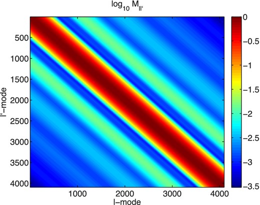
Normalized 3D mixing matrix for the W1 field, the colour scale shows the amplitude of the mixing matrix, and is logarithmic as depicted.
In Kitching et al. (2007) a correction was made to the covariance matrix to account for the very small angular size of the COMBO-17 field. In this paper we do not apply this correction because the survey geometry of the CFHTLenS fields is large enough that the correction factor (|${\mathcal {F}}$|, equation 10 in Kitching et al. 2007) is approximated by a delta function and also that the mixing matrix formalism itself consistently accounts for the survey geometry.
These covariance estimates represent a significant computational task: involving 2 nested sums over the galaxy population, five nested integrals, computation of the matter power spectra, and the matrix sum with the mixing matrix. Previous implementations (Kitching et al. 2007) were prohibitively slow (∼ 1 h per cosmology on a desktop computer in 2007), limitations that have been overcome in the 3dfast implementation (∼ 5 s per cosmology on a desktop computer in 2013; with a parallelized and extendable code) allowing for exploration of large cosmological parameter sets.
2.3 Likelihood
The likelihood of a complex random field in Fourier or spherical harmonic space is more involved than simply treating the real and imaginary parts of the field independently. Here we first describe the covariance matrix for 3D cosmic shear and then define the likelihood function.
2.3.1 The affix-covariance
2.3.2 Likelihood function
In the 3D cosmic shear formalism, which uses a one-point data vector of spherical harmonic coefficients, the covariance itself contains all the cosmological information, and the inverse is exact. Hence there is no need to estimate the covariance itself from data or simulations. When the covariance must be estimated this results (because of the Wishart distribution of the covariance) in the need for calibration with simulations (see e.g. Taylor et al. 2013) to account for the Kaufman/Anderson bias (Kaufman 1967; Anderson 2003; see also Hartlap, Simon & Schneider 2007). For the case of correlation function analyses of the CFHTLenS data Kilbinger et al. (2013) used a hybrid ansatz of a combined analytical and estimated covariance, the former does not need to be corrected for the Kaufman/Anderson bias but the latter does. As discussed in Taylor et al. (2013) one mitigation approach is to use an analytic covariance, as is done in this paper.
An assumption we make here, that the likelihood function is Gaussian, is likely to be incorrect in detail on small scales, but for CFHTLenS this approximation is sufficient. For a survey the size of CFHTLenS we expect to be in the shot noise-dominated regime for any individual ℓ-mode, and one may expect that the shear coefficients will be Gaussian distributed because of the central limit theorem acting through the sum that is performed over the real-space galaxy shear values (that may have a non-Gaussian distribution). As a test of the Gaussianity of the shear coefficients we examine their distribution divided by the expected shot noise (equation 3), what we will refer to as ‘normalized transform coefficients’; which should have a unit Gaussian distribution. We show in Fig. 2 a histogram of the variances, skewnesses and kurtoses of the normalized transform coefficients over all ℓ-modes over all CFHTLenS fields (see Section 3 for a description of the data); we compare this to the expected distribution of these statistics for Gaussian distributed data of this size (for the expected error on the error see Taylor et al. 2013; for the skewnesses see Kendall, Barndorff-Nielson & van Lieshout 1998; for the kurtoses see Kenney & Keeping 1962), and also to a mock realization of the normalized transform coefficients sampled from a unit Gaussian. We find that there is no significant deviation from Gaussianity. We do find that ≲1 per cent of the modes have a small positive excess kurtosis, but due to the overall weak constraints presented in Section 4 this level of non-Gaussianity should not impact results. In Fig. 5 we also show histograms of the normalized transform coefficients for a representative set of ℓ values, and averaged over all ℓ values for information. As a quantitative test of Gaussianity we also perform a Kolmogorov–Smirnov (KS) comparison between the distribution of the transform coefficients and the best-fitting Gaussian, and compare this with Gaussian realizations of the data using the best-fitting values. The results of this KS comparison are shown in Fig. 2, where we again find no significant deviation from Gaussianity, although the KS test is best at detecting a shift in the mean of two distributions.
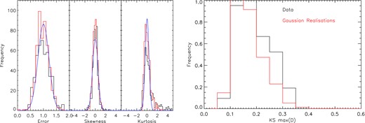
Left: the distribution of standard deviations, skewness and kurtosis for the normalized transform coefficients over all ℓ-modes and for all CFHTLenS fields. We show the distribution of the data (black), the distributions from a Gaussian realization of the data (red) and the analytic expected distribution of these statistics (solid blue lines) for a data set of this size (see Section 3). Right: a normalized histogram of KS supremum values, over all ℓ-modes from all CFHTLenS fields, between the distribution of the normalized transform coefficients and a unit Gaussian distribution (black). We compare this with a similar set of KS supremum values between a unit Gaussian and Gaussian realizations of the data (red), where any difference is due to noise only. These KS supremum value distributions are consistent (with mean values and errors of 0.17 ± 0.06 and 0.21 ± 0.11).
For an isotropic Gaussian field, the harmonic coefficients are statistically independent and normally distributed, where the magnitude of each coefficient provides an independent estimate for the power at the scale of the coefficient (this is where the cosmological constraints stem from in the analysis used in this paper). Isotropy and the high shot noise ensure that the coefficients are close to Gaussian distributed, they have an enhanced variance because of non-linear growth of the power spectrum, and are correlated for different angular modes only through the angular window. All these effects are all included in the analysis, but we make an approximation, in assuming a multivariate Gaussian likelihood, that combinations of coefficients which are uncorrelated are also taken to be statistically independent.
We assume in the likelihood calculation that the data vector of shear coefficients is Gaussian distributed, we do not assume Gaussianity of the shear field itself, as stated before equation (2). Since we use a transform of the field itself, rather than power spectra or correlation functions, the covariance of the data is a 2-point quantity rather than 4-point. We only require isotropy (not Gaussianity) to have a diagonal covariance matrix for the matter power spectrum, and we include non-linearities by using the non-linear power spectrum. With 2-point statistics, the assumption of Gaussianity underestimates the (4-point) covariance, but here this is not the case. Therefore it is sufficient to show that the shear transform coefficients have a Gaussian distribution, and the analysis shows that this is the case, with only very small departures from Gaussianity in the coefficients. The analysis uses the covariance of the shear field as the cosmologically sensitive statistic, hence if the survey area was small this could be sensitive to sample variance whereby local fluctuations could result in an inferred cosmology significantly different from a global description. However because the CFHTLenS survey is a large area, much large than 1 square degree, such sample variance effects are expected to be minimal (e.g. Driver & Robotham 2010).
2.4 Tests on simulations
Despite the fact that the covariance does not need to be estimated from simulations, we nevertheless wished to test the formalism and code to confirm that it was performing as expected. To do this we used the SUNGLASS simulations from Kiessling et al. (2011), which contain shear and redshift probability information assigned on a galaxy-by-galaxy basis, which are ideal for the testing of 3D cosmic shear in principle. For 3D cosmic shear we could not use the CFHTLenS Clone (Harnois-Déraps et al. 2012; used in Benjamin et al. 2013; Heymans et al. 2013, Kilbinger et al. 2013; Simpson et al. 2013, for calibration of the covariance) because the shears were computed in a series of discrete redshift slices not from a full 3D shear field. The SUNGLASS simulations used here consist of 150 realizations of 100 square degrees with a galaxy number density of 16 galaxies per square arcminute with a median redshift of 0.75, and are therefore well matched to CFHTLenS (Heymans et al. 2012) survey characteristics in terms of number density and redshift distribution. The simulations however are smaller in terms of area and do not include an IA model or survey masks, but these are not insurmountable issues and should be addressed in subsequent simulations.
However a more serious limitation is that in analysing these simulations we had to use a limited k and ℓ range. In the radial direction we set a limit7 of k ≤ 1.5 h Mpc−1, by referring to fig. 3 in Kiessling et al. (2011) where it can be seen that the predicted tomographic C(ℓ) begins to deviate from the simulated power at ℓ ≳ 1.5r(zbin) where r(zbin) is the comoving distance of the tomographic bin. Also in Kiessling et al. (2011) a conservative cut in ℓ was used of 500 ≤ ℓ ≤ 1000; this is the regime where the box size (on the large scales) and particle resolution (on the small scales) do not affect the fidelity. The limitations mean that the results of testing on these simulations are expected to give much larger error bars than one should get from data – where larger k and ℓ ranges may be used – which is not limited by simulation resolution effects.
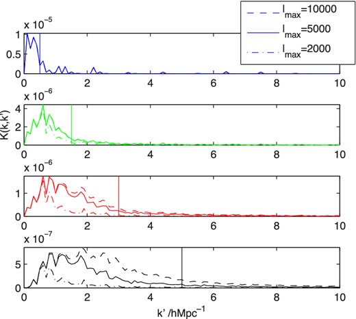
The 3D cosmic shear power spectrum kernel. The four panels show the kernel with which the matter power spectrum is convolved for several k-mode values (shown by vertical lines at values 0.5, 1.5, 3.0 and 5.0 h Mpc−1) in the 3D cosmic shear power. For example the range of k-modes sampled in the matter power spectrum by a k = 0.5 h Mpc−1 value in the 3D cosmic shear power spectrum are shown in the top panel. The range of k-modes sampled depends on the maximum ℓ-mode used, and we show the kernel for three values ℓmax = 2000, 5000 and 10 000. In the cosmological analysis we use kmax = 1.5 h or 5.0 h Mpc−1 and ℓmax = 5000.
We calculated the likelihood surfaces in the (σ8, ΩM) plane over the 150 simulations, over ranges of 0.1 ≤ σ8 ≤ 3.0 and 0.1 ≤ ΩM ≤ 0.9, using the likelihood function described in Section 2.3; all other cosmological parameters were fixed at the values provided in Kiessling et al. (2011), where the simulations used σ8 = 0.8, ΩM = 0.27, ΩB = 0.045, ns = 0.96, and h = 0.71. We find the mean maximum likelihood values in this test are ΩM = 0.27 ± 0.020 and σ8 = 0.82 ± 0.056, which are consistent with the input cosmology. Within the limitations of the simulations available we find that the code and method perform as expected, however we encourage the creation of higher fidelity simulations for further testing; consistency tests are also performed on the CFHTLenS data in Section 3.5.
2.5 Parameter estimation
The cosmological parameter estimation that we will present is performed using a Monte Carlo Markov chain (MCMC) algorithm that uses a Gaussian proposal distribution calculated using the Fisher matrix for the CFHTLenS survey, which uses the same posterior redshift information, survey masks, and ellipticity distributions calculated using a fiducial cosmology centred on WMAP7 (Komatsu et al. 2011) maximum likelihood values. This proposal distribution is efficient because parameter degeneracies are correctly included, however it does assume Gaussianity so no curvature in the likelihood surfaces is captured. The Fisher matrix used is given in Kitching et al. (2011). We create MCMC chains of ≳104 evaluations, and create two chains per cosmology and CFHTLenS field in order to evaluate the Gelman & Rubin (1992) statistic (see Verde 2007 for a clear explanation of this test), which we find to be consistent with the chains having converged for all results presented here.8
3 DATA
The CFHTLenS data and catalogue products are described in Erben et al. (2013), Heymans et al. (2012), Miller et al. (2013) and Hildebrandt et al. (2012). In this analysis we use all four wide fields (W1, W2, W3, W4) and reject pointings based on the Heymans et al. (2012) systematic tests: the tests were performed using a 2D correlation function method which should result in a more stringent rejection because the tests will be sensitive to contaminating effects from all scales, whereas in 3D cosmic shear we reject the smallest scales explicitly from the analysis. We use the catalogues presented in Erben et al. (2013) (the CFHTLenS catalogue) with the shape measurement ellipticities and weights described in Miller et al. (2013), created using lensfit (Miller et al. 2007; Kitching et al. 2008), and the posterior redshift information described in Hildebrandt et al. (2012), created using BPZ (Benítez 2000), which were tested for model fidelity in Benjamin et al. (2013).
The Benjamin et al. (2013) results show that the posterior pg(z) are consistent with the redshift distributions of galaxies with known spectroscopic redshifts, and with redshift distributions reconstructed from a cross-correlation analysis of six photometric redshift bins; we also refer the reader to fig. 5 of Hildebrandt et al. (2012). From this analysis we infer that the set of galaxy template models used in Hildebrandt et al. (2012) are sufficiently complete such that the pg(z) are accurate representations of the true photometric error distribution in the range 0.2 ≤ zBPZ ≤ 1.3. Furthermore Benjamin et al. (2013) based their analysis upon correlation functions. The higher sensitivity of 3D cosmic shear to redshift-dependent effects may be taken to imply that the method would be more sensitive to biases in photometric redshifts, however Kitching et al. (2008) find a similar required error on a global bias for 3D cosmic shear to requirements for weak lensing power spectrum tomography (e.g. Ma et al. 2006). Although the pg(z) were tested in detail in Benjamin et al. (2013) and Hildebrandt et al. (2012), the selection of late-type galaxies to avoid IA in this paper (see Section 3.1) may impact the applicability of those results. However, given the relatively large errors bars, we do not expect this to be significant for this study.
3.1 Galaxy selection
We make a redshift selection of posterior redshift distributions pg(z) of those galaxies with maximum-posterior values between 0.2 ≤ zBPZ ≤ 1.3. This is based on the cross-correlation analysis in Benjamin et al. (2013) who found consistency between spectroscopic and narrow band number densities and the summed pg(z) over these ranges, which is taken as evidence of a low level of infidelity due to model/template error in BPZ. These galaxies have a weighted median redshift of zm = 0.7, and a mean effective number density of 11 galaxies per square arcminute over all fields before any selection.
We make a cut in galaxy type by excluding all galaxies classified as early-type, with a BPZ type parameter TB ≤ 2. The aim of this cut is to create a model-independent removal of galaxies with a large IA signal, based on the analysis of Heymans et al. (2013). However since the linear alignment model (Hirata & Seljak 2004) was used in that analysis there is some model dependence. Mandelbaum et al. (2011) found similar results to Heymans et al. (2013). We will investigate a more sophisticated 3D IA removal in future work (see Merkel & Schäfer 2013, for a theoretical study of IAs within the 3D cosmic shear context).
We use the image masks provided by Erben et al. (2013), and exclude those galaxies with MASK ≥ 2 as described in Erben et al. (2013). We make no other selection of galaxies in the CFHTLenS catalogue. After selection the mean effective number density is 7–8 late-type galaxies per square arcminute over all fields.
3.2 Scales
We test two different ranges of radial scale kmin = 0.001 h Mpc−1 and kmax = 1.5 h Mpc−1 or 5.0 h Mpc−1. The maximum radial scale of 1.5 h Mpc−1 is defined to avoid the highly non-linear regime where baryonic effects are expected to become important (see e.g. White 2004; Zhan & Knox 2004; Jing et al. 2006; Zentner et al. 2008; Kitching & Taylor 2011; Semboloni et al. 2011, 2013; van Daalen et al. 2011; Yang et al. 2013). The halofit (Smith et al. 2003) predictions also become unreliable at a redshift-dependent kmax (Giocoli et al. 2010) at similar scales. The higher scale of 5.0 h Mpc−1 will enable a testing of these assumptions, probing the regime where feedback may be important.
This analysis is much more conservative than the correlation function analyses of the same data (Benjamin et al. 2013; Heymans et al. 2013; Kilbinger et al. 2013; Simpson et al. 2013) where for example a minimum scale of 0.8 arcmin is used, which is equivalent to a data vector cut of k ≤ 27,000/r(z) ≲ 30 h Mpc−1 for the closest redshifts, or k ≲ 10 h Mpc−1 at the median redshift.9 A more conservative correlation function analysis in Kilbinger et al. (2013) uses a minimum scale of 17 arcmin in the data vector but the remaining modes still necessarily contain a mix of information from all physical scales; this is because for a correlation function method the kernel, a Bessel function J0, 4(ℓθ) has significant power at all scales, so a cut in the data vector at a particular scale does not translate into a cut in a physical scale.
For the angular scales we use ℓmin = 360 to avoid any residual systematic effects on scales larger than a single CFHTLenS pointing. To sample the 2D ℓ-space we then create modes ℓx = iℓmin and ℓy = jℓmin (where i, |$j\in {\mathbb {Z}}$|) such that the magnitude of the ℓ vector |$\ell =\scriptstyle\sqrt{\ell _x^2+\ell _y^2}$| is always less than ℓmax = 5000. We use integer multiples of ℓmin for computational reasons, but note that this could limit the signal-to-noise ratio of the final results. We evaluate the data vectors and the theoretical covariance at each point in this 2D space, concatenating those combinations of ℓx and ℓy that give the same ℓ, resulting in 164 independent angular modes. We then sum the likelihood values, equation (9), for parameter estimation. In the radial direction for every ℓ-mode, we use 50 k-modes linearly sampled between 0.001–5.0 h Mpc−1 (therefore 15 for the k ≤ 1.5 h Mpc−1 cut). The MCMC chain is common for all the data, where at each point the log-likelihood is summed over all fields.
3.3 3D cosmic shear power spectra
The 3D cosmic shear power spectra are inherently complex 3D objects in (ℓ, k1, k2) space. In Fig. 4 we show the signal, cosmology dependent, part of the 3D cosmic shear power spectrum in this space. This shows the broad features that lower ℓ-modes contain more power and that as the ℓ-mode increases fewer k-modes are accessible because of the Bessel function behaviour, that we discuss further below.
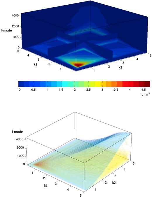
3D representations of the signal part of the 3D cosmic shear power spectra |$C^S_{\ell }(k_1,k_2)$| (equation 2) averaged over the real and imaginary parts. The upper panel shows a slice plot through the 3D (ℓ, k1, k2) space plotted on the z, y and x axes, respectively. The slices/cross-sections through the 3D cube in the top panel are at k = 2.5 h Mpc−1. The lower panel shows the same power spectrum but in an isosurface representation. The colour bar gives the amplitude of the power at each point in the 3D space for both panels.
To present the full 3D power spectrum in a more accessible form we can take conditional cross-sections of this space or make projections. In Fig. 5 we show, for a representative set of ℓ-modes for each field, the diagonal part of the power spectra Cℓ(k, k) and compare this with the square of E-mode data vector values for both the real and imaginary parts of the power spectrum; these quantities should be approximately equivalent if the power spectrum is nearly diagonal in the k direction, we scale the quantities by k2 so that one would have a flat spectrum if there were equal power in each shell in k space. Not all ℓ-modes have both real and imaginary power spectra because of the nature of the complex derivatives (D1 and D2 in equation 2) in the ℓ coordinate system.
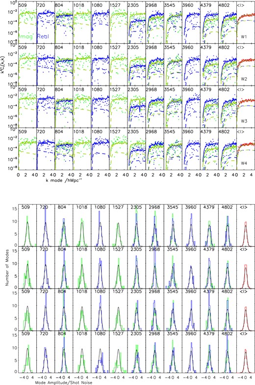
Upper panel: a k-diagonal cross-section through the 3D power spectra. The data points show the real and imaginary values of the transform coefficients squared |$\gamma ^2_E(k,\ell )$| as a function of k for a representative set of 12 ℓ-modes from the ∼164 ℓ-modes computed for each CFHTLenS field: W1, W2, W3 and W4, respectively, from top to bottom in rows. The green points and lines are for the imaginary part, and the blue for the real part. The dashed and solid lines show the diagonal part of the signal and noise covariances, respectively, in the k direction Cℓ(k, k) calculated at a reference WMAP7 cosmology (Komatsu et al. 2011), for the imaginary (green) and real (blue) parts of the covariance. The rightmost column shows the mean of the same cross-section averaged over all ℓ-modes for each field, and averaged over the real and imaginary parts. Lower panel: a histogram of the real (blue) and imaginary (green) shear coefficients for each ℓ-mode in the upper panel, and also averaged over all ℓ-modes, divided by the expected shot noise. The black lines show unit Gaussian distributions.
The dominant feature that one sees in Fig. 5 is the sharp drop in power at low k for each ℓ, which is expected and is due to the Bessel function behaviour jℓ(kr) ≈ 0 for ℓ ≥ kr. In this case for a given k we expect to find power at k ≥ ℓ/rmax ≳ ℓ/(3000zmaxh −1 Mpc). A further clear feature is that for any given (ℓ, k) mode the signal-to-noise ratio of the power spectrum is much less than unity, typically ∼10 per cent (the ratio of the dashed lines to the solid lines in Fig. 5). We note, however, that in total over CFHTLenS we have ∼200 × 50 × 4 ∼ 40 000 independent modes. This is expected for a survey of this size, but since the signal-to-noise ratio increases linearly with the number of galaxies for a particular mode future surveys may even detect individual modes at signal-to-noise ratio greater than unity. We also show the same cross-section in k averaged over all ℓ-modes. The consistency of the shot noise part with the B mode is in agreement with a similar conclusion reached in a mass-mapping analysis of the same data in van Waerbeke et al. (2013).
3.4 2D and tomographic cosmic shear power spectra
A further projection that one can make of the 3D power spectrum is to average over the k-direction to create a purely angle-dependent representation of the power. In Appendix D we show how one can compute such 2D, or tomographic, power spectra from the full 3D case. Using this formalism one could calculate any 2D autocorrelation or cross-correlation power spectrum between any pair of redshift bins.
In Fig. 6 we show the 2D projected power when averaging over the whole redshift range, a ‘2D cosmic shear power spectrum’, for each of the CFHTLenS fields. We show the sum of E-mode power averaged over real and imaginary parts with the shot noise subtracted and compare this to the 2D projected signal calculated with a reference WMAP7 cosmology (Komatsu et al. 2011). Other 2D power spectrum analyses for weak lensing have been presented by Pen, Van Waerbeke & Mellier (2002) using the VIRMOS-DESCART survey, Brown et al. (2003) using the COMBO-17 survey, and Heymans et al. (2005) using the Hubble Space Telescope GEMS survey. We do not combine the fields in our visualizations of the data because such a combination is not a necessity for our analysis; such a combination is also not trivial because the mixing matrices and number density vary between fields. The theory curves plotted are convolved with the mixing matrix, computed from the inhomogeneous and non-smooth masks in the data, and hence are not smooth as may be expected if this was not done.
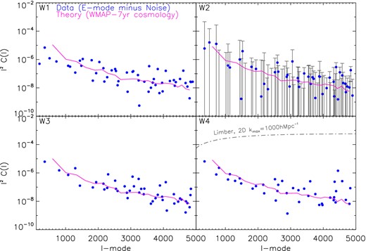
The projected 2D cosmic shear power spectrum for each of the CFHTLenS fields; computed by integrating the full 3D cosmic shear power. The data points show the E-mode only power as a function of ℓ. The solid line shows the 2D power spectra estimates calculated using a reference cosmology of WMAP7 (Komatsu et al. 2011). For the W2 field we show the error bar on each point, which are also typical of the other fields. Because of the logarithmic y axes negative values as a result of noise are not shown. For illustration, in the W4 field only, the grey dot–dashed line shown is the 2D cosmic shear power spectrum that one would compute from data evaluated on a plane, or from theory if no cut in the radial k-direction were imposed in the Limber-approximated calculation.
In Fig. 7 we show a set of tomographic power spectra using both 2 and 6 redshift bins, using the same redshift binning used in Benjamin et al. (2013; 2-bin) and Heymans et al. (2013; 6-bin) for correlation function analyses. We show the intrabin or ‘autocorrelation’ power spectrum for each redshift bin and the interbin or ‘cross-correlation’ power spectrum for each redshift bin combination in the set. It can be seen that the scaling of the data with redshift matches that expected from a WMAP7 cosmology (Komatsu et al. 2011); except in the highest redshift bin where we see some excess of power. There is more power at high-ℓ for high redshifts, which is what one expects, the drop in power is seen at ℓmax ≈ kmaxr(z). The overall drop in power from low to high ℓ is due to the maximum k cut similar to the 2D case (Fig. 6). The smaller amount of interbin power, decreasing as the bin separation increases, is also expected as there is less common lensing material between the bins. Note that this presentation could be extended to an arbitrary number of bins.10 Because the signal-to-noise ratio of the shear transform coefficients is low in CFHTLenS (see Fig. 5) the projected power spectra also have a high level of noise; as a consequence points that are scattered to negative values as a result of noise are not shown in Figs 6 and 7, and we show typical error bars for each point.
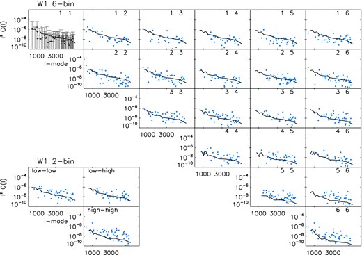
Tomographic power spectra for the CFHTLenS W1 field; computed by integrating the full 3D cosmic shear power. The data points show the summed E-mode power as a function of ℓ. The solid lines show the power spectrum for a WMAP7 (Komatsu et al. 2011) cosmology. The main 21 panels show a 6-bin tomographic set, the numbers refer to the redshift bin combinations where bins 1 to 6 have redshift ranges 0.2 < z ≤ 0.39, 0.39 < z ≤ 0.58, 0.58 < z ≤ 0.72, 0.72 < z ≤ 0.86, 0.86 < z ≤ 1.02, 1.02 < z ≤ 1.30, respectively (the same as Heymans et al. 2013 who present correlation function tomography); the diagonal panels show the intrabin power spectra, the off diagonals the interbin power spectra. The smaller set of 3 panels show a 2-bin tomographic set, the labels low and high refer to the redshift bin combinations where low and high redshift ranges are 0.5 < z ≤ 0.85 and 0.85 < z ≤ 1.30, respectively (the same as Benjamin et al. 2013 who present correlation function tomography). In the first panel we show the error bars on each point, which are typical for the other bins both sets. Because of the logarithmic y axes negative values as a result of noise are not shown.
If one does not use 3D cosmic shear but instead uses 2D or tomographic approximations then it is important to correctly account for the effect that any cuts made in the radial k-modes have on the angular ℓ-modes used in both the theoretical calculation and in the measurement of the power spectra from the data. Cuts in the radial k-modes on the matter power spectrum for example have, as a result of the projections and the Limber approximation, an impact on ℓ-modes in the regime k ≥ ℓ/rmax ≳ ℓ/(3000zmaxh −1 Mpc). Cuts on radial k-modes therefore result in a suppression of 2D or tomographic power at a fixed ℓ-mode as power from the cut modes is removed. This effect is readily computable from theory, either from the full 3D power spectrum or by making tomographic approximations (e.g. Hu 1999; Kitching et al. 2011), and indeed it is necessary to do so because small scales should be removed due to uncertainties in baryonic feedback, and the non-linear power spectrum.
However, the estimation of a 2D power spectrum from data, which consistently removes these modes for a correct comparison to theory, has not been demonstrated until now. In fact the computation of 2D power, from an inherently 3D field, on a plane will contain contributions from all k-modes. In Fig. 6 we represent what one would have computed from data using this procedure, assuming the Limber approximation with no k-mode cut, with the grey dot–dashed line: in this case the data would be orders of magnitude away from the theoretical predictions. One can mitigate this by computing the theoretical power to larger k values, but such a procedure carries uncertainties. If one projects the shear field on to a plane then both the selection function of the galaxies and a correct removal of power from ℓ ≥ kmaxr(z) would have to be performed. Alternatively one can use the full 3D transform coefficients, and use the projection presented in this paper to remove k-modes from the data covariance. A further point is that the k-mode cuts in the data vector translate to a particular kernel with which the matter power spectrum is convolved as discussed in Section 4.2.
3.5 Systematic tests
There are several systematic tests that one can perform, under particular assumptions, to determine whether the power spectra calculated from the data are consistent with expectations.
The B-mode part of the power spectrum should be consistent with shot noise only (equation 3), because cosmic shear only induces E-mode power. Therefore the B-mode power minus the expected shot noise power spectrum should be consistent with zero. This assumption can break down due to IAs (see e.g. Merkel & Schäfer 2013), but at the level of precision attainable from CFHTLenS, and the fact that we remove the galaxies that are most likely to be contaminated with IAs, this is a valid systematic test.
The cross power spectrum between the E and the B-mode power should be consistent with zero. A non-zero E–B power spectrum would correspond to a mixing of E- and B-mode power which is expected to be zero, except in some exotic cosmologies (see Amendola et al. 2013 for a review), or as a result of residual systematic B-mode power being mixed with the E-mode power through the application of the mixing matrix.
- For a Gaussian random field the phase of the E- and B-mode power spectra for a given mode isThe distribution of phases should be random, and consistent with a uniform distribution over [0, 2π] (see Coles et al. 2004 for a study of phases in a CMB study) if there is no preferred direction in the data (this tests sensitivity to a shift in the origin of the coordinate system used). The shear coefficients used in the above equation are the observed shear coefficients (equation A8 in Appendix A) to test the isotropy of the on-sky shear field.(11)\begin{equation} \phi ={\rm atan}\left(\frac{{\mathbb {I}}[\gamma (k,\ell )]}{{\mathbb {R}}[\gamma (k,\ell )]}\right). \end{equation}
We show the result of the first two of these systematic tests in Fig. 8 for each of the four fields as a function of ℓ, averaged over k, and the real and imaginary parts of the power spectra. We find that as expected each of these tests is consistent with zero.
![Upper panels: for each of the CFHTLenS fields we show the shot noise subtracted B-mode power (blue points) and the EB cross power spectra (orange points) Each of these should be consistent with zero. We have binned the ℓ-modes into 6 bins and show the error bar associated with each; we have shifted the B-mode by a small amount away from the bin centre (used for the EB points) in ℓ for clarity in plotting. Lower panels: for each of the CFHTLenS fields we show a histogram of the complex phase of the observed shear coefficients (equation 11). Each of these should be consistent with a uniform distribution over the range [0, 2π], if the data are isotropic. The solid horizontal line shows the expected mean number of modes per bin, and the dashed lines show the expected 1σ error.](https://oup.silverchair-cdn.com/oup/backfile/Content_public/Journal/mnras/442/2/10.1093/mnras/stu934/2/m_stu934fig8.jpeg?Expires=1749936222&Signature=XhXxs2A64BMpNGB3lkvFqGM5Jj6f--0jdBpPOaqzgLEeJwKpgYRLqzihlIwhwVLJIcr-QsxfBCQa~GusCbTxAz4orSbL5zukPRZAfKvRlIlRm33fYUmxIQv7UUiE4hZYRpPr2o2TaEMXC8~Zdcyl~TFgg~WvM1wbsskHYIKYmhE9Mvap6S2sHSFKAYvPqpWkOSK5MCxCARmUVlVkN8LKZ53PJqMoARknPs2U1rl6EfP73sc33Lc8WwAbS7x71sgkKtDyIWc2sw-4z2lysJ4niYQ5o2Ns4La5JlvFNNawXCURaR9zMZKlZgOacFhKRH~N8BqOheP8kbml4afG5hMTkA__&Key-Pair-Id=APKAIE5G5CRDK6RD3PGA)
Upper panels: for each of the CFHTLenS fields we show the shot noise subtracted B-mode power (blue points) and the EB cross power spectra (orange points) Each of these should be consistent with zero. We have binned the ℓ-modes into 6 bins and show the error bar associated with each; we have shifted the B-mode by a small amount away from the bin centre (used for the EB points) in ℓ for clarity in plotting. Lower panels: for each of the CFHTLenS fields we show a histogram of the complex phase of the observed shear coefficients (equation 11). Each of these should be consistent with a uniform distribution over the range [0, 2π], if the data are isotropic. The solid horizontal line shows the expected mean number of modes per bin, and the dashed lines show the expected 1σ error.
In Fig. 8 we also show the distribution of the complex phases of the observed transform coefficients averaged over all ℓ and k-modes, which we find to be consistent with a uniform distribution for each field.
4 RESULTS
We now present the cosmological parameter constraints found from 3D cosmic shear applied to the CFHTLenS data. The cosmological parameter set we use is a waCDM set with ΩM, ΩB, σ8, h , w0, wa, ns with others fixed at WMAP7 maximum likelihood values (Komatsu et al. 2011), we also assume flatness i.e. ΩDE = 1 − ΩM, and a sum of neutrino mass of zero. We also consider a wCDM parameter set where wa = 0, and a Lambda cold dark matter (LCDM) parameter set where w0 = −1 and wa = 0. Constraints on other cosmological parameters are expected to be dominated by CMB constraints for this size of lensing survey, except possibly the neutrino mass. The dark energy equation of state is parametrized using a Taylor expansion in scale factor such that w(z) = w0 + [z/(1 + z)]wa.
4.1 Priors
We will present the 3D cosmic shear parameter error in combinations with priors from previously analysed cosmological data sets. These are as follows.
Planck. We include constraints from the Planck 1st year data. See Planck Collaboration (2013) and the PLAIO11 for a description of the data products. We use the lowl_lowLike chains and for the waCDM parameter set use the combination of Planck+BAO.
h 0. The constraint on the dimensionless Hubble parameter h = H0/(100 km s− 1Mpc− 1) = 0.738 ± 0.024 from Riess et al. (2011). We apply this assuming a Gaussian prior distribution.
WMAP7+SN+BAO. We include results from Komatsu et al. (2011) for the CMB in combination with priors used in that analysis.12 We use the MCMC chains made available subsequently13that also include information from the Hicken et al. (2009) supernovae data set (+SN) and BAO information from Percival et al. (2010) (+BAO).
The WMAP7+SN priors we use do not contain systematic errors on the supernovae constraints. This is addressed in Conley et al. (2011) who find that the combined WMAP7+SN constraints including systematic are not biased with regard to Komatsu et al. (2011) (due to the orthogonality of the CMB and Type Ia SN contours even when including systematics), but that uncertainties from SN alone are increased by a factor of 2. Komatsu et al. (2011) included an h 0 prior from Riess et al. (2009) of h = 0.742 ± 0.036, and we modify the weights of the WMAP7 MCMC chains to remove the Riess et al. (2009) h 0 prior and include the Riess et al. (2011) h 0 prior for this paper. In addition we include some physical priors ΩM > 0, ΩB > 0, h > 0, σ8 > 0 to prevent the MCMC chains from moving into unphysical parts of parameter space. We also include (i) the same uniform priors as Kilbinger et al. (2013) of ΩB ∈ [0.0; 0.1], ns ∈ [0.7; 1.2] and (ii) some priors that result from the stability of camb, where we exclude the ranges ΩM < 0.05, h < 0.1 and (w0 > −0.5∧wa > 0.8) (see Appendix E).
4.2 Scales
In Fig. 9 we show constraints in the (σ8, ΩM) plane for two different ranges in scale. In this projection we find that results are consistent when the maximum k is increased from 1.5 to 5.0 h Mpc−1, but we will see tension later when combined with Planck. Moreover even over this small change in scale a lower σ8 is preferred as the maximum k increases. We show numerical results for a fit to the function σ8(ΩM/0.27)α = constant in Table 1 where we find that the normalization is affected by a change in scale but that the slope is unaffected.
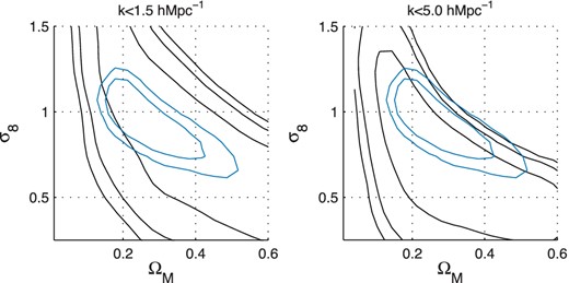
Constraints in the (σ8, ΩM) plane for a wCDM cosmology as a function of the range in k-modes used in the analysis (black contours). We show the wCDM WMAP 7 yr contours (blue inner lines) for comparison. Contours shown are 2-parameter 1 and 2σ confidence regions. In the left-hand panel the k range is k ≤ 1.5 h Mpc−1; and in the right-hand panel for k ≤ 5.0 h Mpc−1
The mean parameter values from an CFHTLenS 3D cosmic shear analysis (this paper) and we quote numbers from 1-bin 2D correlation function analysis (†Kilbinger et al. 2013, tables 2 and 3) and 6-bin tomographic correlation function analysis (‡Heymans et al 2013, tables 2 and 3). The upper rows show the lensing-only constraints on the empirical relation σ8(ΩM/0.27)α =constant, that parametrizes the amplitude and width of the (σ8, ΩM) contour; see Heymans et al. (2013) table 2 for further values of these under various assumptions in a ΛCDM cosmology. The lower rows compare the constraints in a flat wCDM cosmology, with lensing combined with WMAP7. For the 3D cosmic shear only constraints we quote asymmetric error bars. Note that Heymans et al. (2013) also marginalized over an IA parameter A, but included 1.5 times as many galaxies. The errors are symmetric 1-parameter 1σ values. *Have no allowance for baryonic feedback effects that are likely to impact constraints using k ≳ 1.5 h Mpc−1.
| Parameter | flat LCDM Lensing only | Analysis and Method | |
|---|---|---|---|
| α | |$0.44^{+0.24}_{-0.36}$| | 3D cosmic shear power spectra | k ≤ 1.5 h Mpc−1, no early-type galaxies |
| |$0.46^{+0.37}_{-0.36}$| | 3D cosmic shear power spectra* | k ≤ 5.0 h Mpc−1, no early-type galaxies | |
| 0.59 ± 0.02 | 1-bin correlation function† | k ≲ 30 h Mpc−1, all galaxies | |
| 0.46 ± 0.02 | 6-bin correlation function† | A marginalized, k ≲ 30 h Mpc−1, all galaxies | |
| σ8(ΩM/0.27)α | |$1.16^{+0.27}_{-0.27}$| | 3D cosmic shear power spectra | k ≤ 1.5 h Mpc−1, no early-type galaxies |
| |$0.69^{+0.22}_{-0.22}$| | 3D cosmic shear power spectra* | k ≤ 5.0 h Mpc−1, no early-type galaxies | |
| 0.79 ± 0.04 | 1-bin correlation function† | k ≲ 30 h Mpc−1, all galaxies | |
| |$0.77^{+0.03}_{-0.04}$| | 6-bin correlation function‡ | A marginalized, k ≲ 30 h Mpc−1, all galaxies | |
| flat wLCDM Lensing only | |||
| α | |$0.46^{+0.23}_{-0.26}$| | 3D cosmic shear power spectra | k ≤ 1.5 h Mpc−1, no early-type galaxies |
| |$0.39^{+0.50}_{-0.29}$| | 3D cosmic shear power spectra* | k ≤ 5.0 h Mpc−1, no early-type galaxies | |
| 0.59 ± 0.03 | 1-bin correlation function† | k ≲ 30 h Mpc−1, all galaxies | |
| σ8(ΩM/0.27)α | |$1.14^{+0.26}_{-0.30}$| | 3D cosmic shear power spectra | k ≤ 1.5 h Mpc−1, no early-type galaxies |
| |$0.72^{+0.30}_{-0.30}$| | 3D cosmic shear power spectra* | k ≤ 5.0 h Mpc−1, no early-type galaxies | |
| 0.79 ± 0.07 | 1-bin correlation function† | k ≲ 30 h Mpc−1, all galaxies | |
| w | |$-1.40^{+1.30}_{-0.82}$| | 3D cosmic shear power spectra | k ≤ 1.5 h Mpc−1, no early-type galaxies |
| |$-1.41^{+1.25}_{-0.80}$| | 3D cosmic shear power spectra* | k ≤ 5.0 h Mpc−1, no early-type galaxies | |
| |$-1.17^{+0.80}_{-1.40}$| | 1-bin correlation function† | k ≲ 30 h Mpc−1, all galaxies | |
| flat wCDM Lensing+WMAP7 | |||
| ΩM | 0.252 ± 0.079 | 3D cosmic shear power spectra | k ≤ 1.5 h Mpc−1, no early-type galaxies |
| 0.210 ± 0.069 | 3D cosmic shear power spectra* | k ≤ 5.0 h Mpc−1, no early-type galaxies | |
| 0.325 ± 0.082 | 1-bin correlation function† | k ≲ 30 h Mpc−1, all galaxies | |
| 0.256 ± 0.110 | 6-bin correlation function‡ | A marginalized, k ≲ 30 h Mpc−1, all galaxies | |
| σ8 | 0.88 ± 0.23 | 3D cosmic shear power spectra | k ≤ 1.5 h Mpc−1, no early-type galaxies |
| 0.88 ± 0.22 | 3D cosmic shear power spectra* | k ≤ 5.0 h Mpc−1, no early-type galaxies | |
| 0.77 ± 0.11 | 1-bin correlation function† | k ≲ 30 h Mpc−1, all galaxies | |
| 0.81 ± 0.10 | 6-bin correlation function‡ | A marginalized, k ≲ 30 h Mpc−1, all galaxies | |
| w | −1.16 ± 0.38 | 3D cosmic shear power spectra | k ≤ 1.5 h Mpc−1, no early-type galaxies |
| −1.23 ± 0.34 | 3D cosmic shear power spectra* | k ≤ 5.0 h Mpc−1, no early-type galaxies | |
| −0.86 ± 0.22 | 1-bin correlation function† | k ≲ 30 h Mpc−1, all galaxies | |
| −1.05 ± 0.34 | 6-bin correlation function‡ | A marginalized, k ≲ 30 h Mpc−1, all galaxies | |
| h | 0.78 ± 0.12 | 3D cosmic shear power spectra | k ≤ 1.5 h Mpc−1, no early-type galaxies |
| 0.83 ± 0.12 | 3D cosmic shear power spectra* | k ≤ 5.0 h Mpc−1, no early-type galaxies | |
| 0.66 ± 0.11 | 1-bin correlation function† | k ≲ 30 h Mpc−1, all galaxies | |
| 0.74 ± 0.14 | 6-bin correlation function‡ | A marginalized, k ≲ 30 h Mpc−1, all galaxies |

Constraints in the (σ8, ΩM) plane for a wCDM cosmology for k ≤ 5.0 h Mpc−1, including the functional ansatz from van Daalen et al. (2011) and Semboloni et al. (2011, 2013) for the effect of baryonic feedback on the matter power spectrum, that we parametrize in equation (12). The left-hand panel reproduces the plot from Fig. 9 for comparison; the middle panel shows the constraints using the functional ansatz predicted, with no amplitude change ES = 1; the right-hand panel shows the constraints when using a power spectrum that is damped three times more than that predicted ES = 3. We show the wCDM WMAP 7 yr contours (blue inner contours) for comparison.
4.3 wCDM cosmologies
Here we explore the combination of CMB constraints with those from lensing in comparison with similar combinations from other cosmological probes in the wCDM parameter space. The CMB alone (not accounting for lensing of the CMB) suffers from a geometric degeneracy which means the constraints are large in particular parameter directions, in particular for ΩM, h and w. CMB measurements alone can lift the degeneracy to some degree with CMB lensing and the ISW effect, but are generally combined with other cosmological probes in order to take full advantage of the statistical power of additional data sets.
Figs 11, 12 and Table 1 clearly show that lensing can provide an independent way to lift CMB degeneracies, to a degree comparable with current h 0 constraints and the combination of BAO+SN, in particular for σ8 and the dark energy equation of state w; but this depends on the range of scales used. Using scales of k ≤ 1.5 h Mpc−1 only we find that the lensing data does not add any significant constraining power to the CMB data. However, when using scales of k ≤ 5 h Mpc−1, and no baryonic feedback correction, the tension between the slightly lower σ8 and ΩM cause the CMB degeneracies to be lifted, but the posterior is driven to very low ΩM ≲ 0.2, high h ≳ 0.8 and high σ8 ≳ 1.
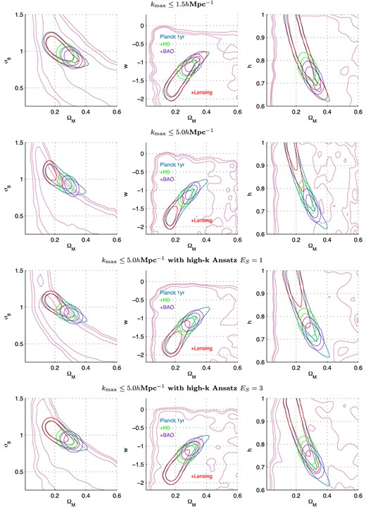
The combination of Planck CMB data with the 3D cosmic shear constraints (Lensing; red contours), compared to the combination of Planck with BAO (Percival et al. 2010; purple contours) and with h 0 (Riess et al. 2011; green contours). We show three projected 2-parameter spaces in a wCDM cosmology, where wa = 0. Contours shown are 2-parameter 1 and 2σ confidence regions, pink contours show the lensing-only constraints. Note that the absence of power suppression in the range 1.5 < k ≤ 5.0 h Mpc−1, such as may be provided by AGN feedback results in the posterior being driven to ΩM ≲ 0.2, w ≲ 1.5, h ≳ 0.8 and σ8 ≳ 1.0 for the k < 5.0 h Mpc−1 results. The lower two rows include the high-k functional ansatz discussed in Section 4.2.
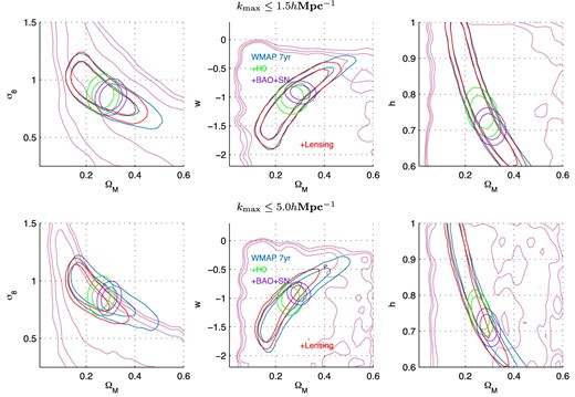
As the top two rows in Fig. 11 but in combination with WMAP7 priors.
This is evidence of the modelling of the non-linear scales being in tension with the modelling of linear scales, or the presence of an undetected scale-dependent systematic effect. The modelling of the non-linear clustering, either dark matter or baryonic feedback are possible sources of plausibly incorrect modelling (see Section 4.2). Alternatively a cosmological model assuming w = −1 is not correct or needs an additional component: one possible assumption that could be relaxed is that of no massive neutrino species, which could cause a suppression of power at scales >1.5 h Mpc−1 (see Jimenez et al. 2010). This result is unlikely to be caused by residual IA contamination, because such an effect is expected to impact all scales, but this is a further possibility. At the current time the data, and modelling of the baryonic feedback, are not sufficient to confidently distinguish these possibilities; although one, or more, of these must be causing the observed effect. As shown in Fig. 11 , we find that when the high-k functional ansatz described in Section 4.2 is included that the lensing constraints are more consistent with the Planck constraints, and that the degeneracy lifting is relaxed.
4.4 LCDM and waCDM cosmologies
In Fig. 13 we show the 2-parameter projected constraints for the waCDM set with a kmax = 5.0 h Mpc−1, in each of the 2-parameter combinations that are accessible in this analyses.15 It is clear from Fig. 13 that lensing is providing constraints consistent with Planck+BAO for waCDM cosmologies, but that there is very little gain over these, even at the 1σ level. In the waCDM parameter space the constraints from lensing are very broad as the data is not sufficient to place tight constraints in such a larger parameter space.
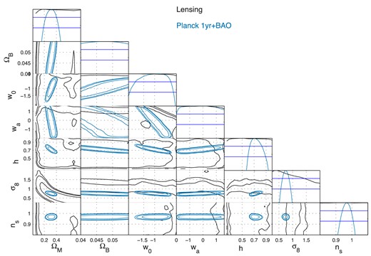
The cosmological parameter constraints from 3D cosmic shear in the waCDM parameter space with kmax = 5.0 h Mpc−1, with no baryonic feedback model included. We show each projected 2-parameter combination accessible in this analysis, with the 2-parameter 1σ, 2σ and 3σ confidence regions shown. Shown are lensing (3D cosmic shear) (black) and Planck+BAO constraints (blue; for waCDM, respectively). We also show the projected 1-parameter likelihoods for each parameter (the top-most blue and black lines). See Section 4.4 for a discussion of this figure.
In the LCDM parameter space the CMB alone already constrains most parameters very tightly – the significant geometric degeneracy in the CMB being lifted by the choice of a cosmological parameter set that assumes flatness – and so similarly we find that there is no tension with the Planck results, but also no improvement with the addition of the CFHTLenS constraints. For comparison we find that for an LCDM cosmology σ8(ΩM/0.27)0.69 ± 0.22 = 1.16 ± 0.27 compared to Planck who find σ8(ΩM/0.27)0.46 = 0.89 ± 0.03 using the same cosmology.
4.5 Comparison with 2D correlation function analyses
Comparing these constraints with those from 2D and tomographic correlation function analysis of the CFHTLenS data (Benjamin et al. 2013; Heymans et al. 2013; Kilbinger et al. 2013; Simpson et al. 2013) we find similar constraints from the full 3D analysis on some parameters, for example w (+1.30 − 0.82 in this paper compared to approximately ±1.0 in Kilbinger et al. 2013 for lensing alone), despite the fact that we only probe 5 per cent to 16 per cent of the modes in the matter power spectrum, and ∼20 per cent fewer galaxies: we use k ≤ 1.5 or 5.0 h Mpc−1 compared to k ≲ 30 h Mpc−1 (see Section 4.2), however this difference results in some subtlety in the comparison that we describe here.
In Table 1 we show constraints on the empirical relation σ8(ΩM/0.27)α = constant, commonly used to parametrize the amplitude and width of the contours in the (σ8, ΩM) plane. We find weaker constraints in the orthogonal direction parametrized by α (width of the contour, as can be seen by comparing Fig. 13 of this paper with figs 11 and 5 of Kilbinger et al. (2013) and Heymans et al. (2013), respectively, for wCDM and LCDM cosmologies) and on σ8. 2D correlation functions constrain a long and thin contour in the (σ8, ΩM) plane, and the conservative 3D cosmic shear constraints presented in this paper are wider, however some marginalized quantities are determined better by one method, some by the other. One may expect simple amplitude changes in the lensing signal (such as changes in the orthogonal direction, or σ8) to be measured more accurately for the correlation function analyses, due to the much larger number of k-modes analysed; and this is supported by the decrease in the error as we increase the number of k-modes in the 3D cosmic shear analysis. However other effects, like shape changes in the linear part of the power spectrum (determined by combinations such as ΩMh 2) and parameters that change the redshift evolution of the matter power spectrum or the expansion history such as w, are more well resolved by 3D cosmic shear at all redshifts. Hence comparable constraints are expected on these parameters, and in combination with CMB constraints, even with a smaller number of total k-modes. We find similar constraints on w comparing 2D correlation function analyses and 3D cosmic shear indicating that the extra constraining power from including small angular scales in the 2D analysis compensates for the constraining power lost by not analysing the data fully in 3D. The tighter constraints on ΩM, h , w also help, through lifting degeneracies, in measuring other parameters in combination with CMB constraints for example σ8. We also find a higher value of σ8 than the correlation function analyses, although results are consistent at the ∼1σ level. In these comparisons the scale dependence of the power, and the modelling uncertainties at high k values, described in Section 4.2 should be considered.
Finally we note here a further aspect that may contribute to the differences with 2D and tomographic analyses. The approach of using the analytic covariance (and one-point estimator) in this paper does not suffer from noise due to finite number of simulations: the 1656 independent lines of sight in the CFHTLenS clone (Harnois-Déraps et al. 2012) and the 210 data points used in Heymans et al. (2013) leads to a ≃4 per cent fractional error on the inverse covariance in their study (using the scaling of Taylor et al. 2013), an error that is not present in the 3D cosmic shear analysis presented here; this error could be considered as a lower bound since any other sources of error or bias in the simulations would not be captured in this number.
A more quantitative comparison of 2D correlation function methodology and 3D power spectrum analysis is more complicated and beyond the scope of this paper; our aim is to present the 3D cosmic shear results, not to perform a close and comprehensive 2D correlation function to 3D power spectrum comparison. In particular for a close comparison with Kilbinger et al. (2013) there are several differences in their analysis that would have to be considered. For example a different galaxy selection was made, different ranges in scale were used.
4.6 Comparison with expected constraints
The constraints from lensing alone presented in this paper are conservative in that we remove galaxies that have evidence for an IA signal, and we remove scales for which there exist uncertainties in the non-linear modelling of the matter power spectrum. However, we can predict the expected constraints using such conservative assumptions and galaxy selections using the Fisher matrix formalism (Kitching, Heavens & Miller 2011; which is also used as the proposal distribution for the MCMC chains in this paper). We find that the most tightly constrained plane is in the projected (σ8, ΩM) direction; see Fig. 13, that can be parametrized by σ8(ΩM/0.27)α = constant. In Fig. 14 we show the measured and predicted constraints on the parameters α and ΩM marginalizing over all other parameters in the wCDM parameter set.
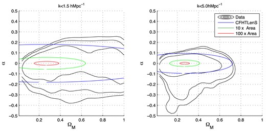
The constraints from CFHTLenS 3D cosmic shear only in the (α, ΩM) plane marginalized over the other parameters in the wCDM parameter set. This is the plane in which the constraints in the projected (σ8, ΩM) plane are uncorrelated, which is parametrized by the function σ8(ΩM/0.27)α = constant. The black contours show the 1σ, 2σ, 3σ constraints from the data, the blue lines show the expected 1σ two-parameter projected constraints in this plane from a Fisher matrix analysis for CFHTLenS, the green and red lines show the expected constraints for a survey 10 times larger area and 100 times larger in area, respectively, with all other survey characteristics kept constant.
We find that the expected 1σ contours coincide with the measured constraints. Therefore the analysis, whilst conservative in its assumptions which leads to broad constraints, is as expected for a survey the size of CFHTLenS. We also show predictions for surveys that are 10 and 100 times the area of CFHTLenS, keeping all other survey characteristics the same, for which we expect significant gains.
5 CONCLUSIONS
In this paper we present the first application of the 3D cosmic shear method to a wide-field weak lensing survey, CFHTLenS (Heymans et al. 2012; Erben et al. 2013) and use this method to measure cosmological parameters including the dark energy equation of state parameters w0 and wa. The CFHTLenS data covers 154 square degrees, of which 61 per cent is unmasked and passes systematics tests, and has been analysed with the state of art in shape measurement (lensfit; Miller et al. 2013) and redshift estimation (BPZ; Hildebrandt et al. 2012).
3D cosmic shear, which uses the covariance of the 3D spherical harmonic/spherical Bessel coefficients of the shear field as its signal, has a number of useful features over other approaches in that (i) it does not bin the data, in particular in the redshift direction along which discoveries of redshift-dependent effects may be found (i.e. dark energy), (ii) it allows for a control of the angular (ℓ) and radial (k) modes in the analysis independently which means that non-linear modes in the matter power spectrum may be explicitly excluded, (iii) it allows for extra information from individual galaxies to be used, for example the posterior information in redshift and (iv) it uses a one-point estimator with an analytic covariance estimate, and hence in this analysis is not sensitive to estimating the inverse covariance from simulations. To account for angular masks in the analysis we present a pseudo-Cℓ method for 3D fields and apply this to the analytic covariance. This is the first application of a pseudo-Cℓ method on weak lensing data: previously mask window functions have been computed for the galaxy power spectrum in Pen et al. (2003) and were not taken into account in Brown et al. (2003), Heymans et al. (2005) or Kitching et al. (2007).
One can project the shear field on to 2D planes in redshift, to create tomographic slices, and in this paper (and in Kitching et al. 2011) we show how 2D and tomographic power spectra can be recovered from the full 3D shear field. Here we apply this and present 2D and tomographic cosmic shear C(ℓ) power spectra (the first presentation of a tomographic cosmic shear power spectrum from data). To reduce IA systematics we exclude all galaxies with BPZ parameter TB ≤ 2 (this preferentially selects late-type galaxies). In the future mitigation techniques should be developed to either remove or account for IAs. 3D cosmic shear uses the redshift posterior probabilities for each galaxy pg(z) in the estimator. We justify our use of the pg(z) on the analysis of Benjamin et al. (2013) who found that the redshift probability distributions were unbiased with respect to a spectroscopic sample of the same galaxies, however that analysis used a correlation function technique, in only 6 redshift bins and for all galaxies in the CFHTLenS catalogue. This means that it probed much smaller scales than in this paper, averaged over all galaxy types, and used a much coarser redshift sampling. In future the determination of the fidelity of redshift posterior information should be performed over scales, and with a redshift sampling, matched to those used in any 3D cosmic shear analysis.
The results we find are not formally in conflict with previous correlation function (configuration space) analyses of CFHTLenS (Benjamin et al. 2013; Heymans et al. 2013; Kilbinger et al. 2013; Simpson et al. 2013). The most interesting finding we have comes from the ability of 3D cosmic shear to probe rather well-defined ranges of physical wavenumber. For wCDM cosmologies we find evidence that there is tension between the lensing constraints that only use scales k ≤ 1.5 h Mpc−1 and those that use k ≤ 5 h Mpc−1, where the lensing at smaller scales (higher k) prefers a lower value of σ8. Taken at face value in combination with either Planck or WMAP7 CMB priors the smaller scales lift the CMB degeneracy and favour w ≲ −1.5, a high value of h ≳ 0.8, a low ΩM ≲ 0.2 and a high σ8 ≳ 1.0 in comparison to concordance LCDM values. This is evidence of either the non-linear modelling being in tension with the linear model, and/or the cosmological model having a deviation from the concordance LCDM: possible explanations include the effects of AGN feedback on the non-linear matter power spectrum (see Semboloni et al. 2011, 2013; van Daalen et al. 2011), or an additional component (e.g. a massive neutrino species) that can suppress power at small scales. We find that when we include a functional ansatz that models the damping of the matter power spectrum due to AGN feedback on scales k ≳ 1.5 h Mpc−1, that the cosmological constraints for the two different ranges of scale are in better agreement. We leave a full investigation of these possible effects for future work, but note that one or more of these explanations is required to explain this observation.
We thank Dipak Munshi, Andy Taylor, Fergus Simpson, Stephen Feeney, Hiranya Peiris, Licia Verde, Raul Jimenez, Jason McEwen and Mark Cropper for useful discussions. We thank Anthony Lewis and the developers of camb, and the PPF module for making their code public. We thank Eric Tittley and Mark Holliman for system administration on several machines used in this work. We made use of CosmoCalc http://www.astro.ucla.edu/wright/CosmoCalc.html (Wright 2006) during development. We thank WMAP for providing their MCMC chains available for download http://lambda.gsfc.nasa.gov, and Eiichiro Komatsu for providing supplementary data products to the main WMAP data release. We thank ESA Planck for providing their MCMC chains available for download http://pla.esac.esa.int/pla/aio/planckProducts.html. TDK acknowledges support from a Royal Society University Research Fellowship.
We refer to Heymans et al. (2013), and Fu et al. (2014) for a full list of acknowledgments for CFHTLenS.
Author Contributions: All authors contributed to the development and writing of this paper. The authorship list reflects the lead authors of this paper (TDK, AFH) followed by two alphabetical groups. The first alphabetical group includes key contributors to the science analysis and interpretation in this paper, the founding core team and those whose long-term significant effort produced the final CFHTLenS data product. The second group covers members of the CFHTLenS team who made a significant contribution to either the project, this paper, or both. The CFHTLenS collaboration was coled by CH and LVW. The CFHTLenS Cosmology Working Group was led by TDK.
The word tomography, meaning a cross-section, slice or image of a predetermined plane in the body, is used colloquially in weak lensing to refer to the power spectra of projected planes integrated along the line of sight.
The software used in this paper, 3dfast, that includes the 3D cosmic shear estimators and parameter estimation, is available on request, and more details are available here http://www.thomaskitching.net
http://camb.info version 2012 October
Affix is a word that can refer to a complex number (Whittaker & Watson 1990), but it also means ‘fasten’ or ‘attach’.
We will use the same limit for the data analysis, but this is a coincidence.
MCMC chains are available on request.
See Benjamin et al. (2013) section 4 for a more thorough discussion of this k-cut for correlation function analyses; however much larger k-modes will contribute to the interpretation of these because of the very broad kernel used in this analysis (Bessel functions J0, 4[ℓθ]). Here we quote the maximum scale in the data vector that is used in the likelihood function in such an analysis, for comparison with the k-cuts used in this paper.
However ultimately limited by the number of galaxies in the survey. Decreased photometric redshift precision would increase correlation between bins but would not limit the number of bins.
We use WMAP7 for consistency with other CFHTLenS results, and Planck for current constraints, we also refer the reader to WMAP9 (Hinshaw et al. 2013) for a further CMB data set that could also be used.
Available here http://gyudon.as.utexas.edu/komatsu/wmap7/ and here http://gyudon.as.utexas.edu/komatsu/wmap7/wacdm+lz/wmap7+h0+snconst/ for the waCDM parameter set and from here http://lambda.gsfc.nasa.gov/product/map/dr4/parameters.cfm for the wCDM parameter set.
However it is not clear whether material blown out by AGN activity may, or may not, be able fall back into its original environment.
We note that the predictions of Kitching (2007) are consistent with the constraints presented here – although the realized survey geometry, number density and depth were not considered explicitly.
REFERENCES
APPENDIX A: E- AND B-MODE SEPARATION
In Kitching et al. (2007) there was no attempt made to split the shear estimators into E- and B-mode parts, in analogy to the procedure that is followed for correlation function analysis. We show here how to correctly link the raw calculated spherical harmonic coefficients into those that can be used to compute E- and B-mode power.
APPENDIX B: THE IMPACT OF SHAPE MEASUREMENT BIAS
The shape measurement correction found by Heymans et al. (2013) (that needs to be applied to the data vector after the measurement process) is a scalar function, and is defined for each galaxy individually, mg. Therefore, it acts in a similar way as a position and redshift-dependent weight map or mask. Here we show how to construct unbiased 3D shear coefficients using such a function.
APPENDIX C: PSEUDO-ESTIMATORS IN 3D
This appendix is based on the formalism first presented in Munshi et al. (2011), we reproduce the derivation here to match to the notation used for the covariance and adopt a flat sky approximation. We show here how a mixing matrix can be defined that, in a forward convolution with the analytic covariance, results in a ‘pseudo’-covariance estimate that now accounts for angular masks in a survey.
We find that the mask only mixes ℓ-modes in the signal part of the covariance, not the shot noise part which is only affected through an area scaling. This can be shown following the derivation of the shot noise covariance in Kitching (2007).
APPENDIX D: 2D POWER FROM 3D POWER
Here we show how 2D and tomographic cosmic shear power spectra can be calculated from the full 3D cosmic shear power spectrum Cℓ(k, k′).
APPENDIX E: camb PRIORS
In this section we present a test of the software camb used in this paper (2012 October, with the PPF module), which was used to justify some of the prior ranges used. We sampled the waCDM parameter space on a grid containing 57 points (five in each parameter direction), in Fig. E1 we show the projected fraction of these points that did not return a matter power spectrum. This functionality is reproduced by a very simple prior: ΩM < 0.05∨h < 0.1∨(w0 > −0.5∧wa > 0.8).
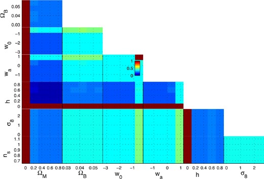
The projected fraction of points from a 57 grid that did not return a matter power spectrum from camb (2012 October, with PPF module). The colour scale in the (w0, wa) projected plane, that displays the colour associated with the fraction, is applicable to all other projections.
