


Abstract
We present a new version of the fast star cluster evolution code Evolve Me A Cluster of StarS (emacss). While previous versions of emacss reproduced clusters of single-mass stars, this version models clusters with an evolving stellar content. Stellar evolution dominates early evolution, and leads to: (1) reduction of the mean mass of stars due to the mass loss of high-mass stars; (2) expansion of the half-mass radius; (3) for (nearly) Roche Volume filling clusters, the induced escape of stars. Once sufficient relaxation has occurred (≃10 relaxation times-scales), clusters reach a second, ‘balanced’ state whereby the core releases energy as required by the cluster as a whole. In this state: (1) stars escape due to tidal effects faster than before balanced evolution; (2) the half-mass radius expands or contracts depending on the Roche volume filling factor; and (3) the mean mass of stars increases due to the preferential ejection of low-mass stars. We compare the emacss results of several cluster properties against N-body simulations of clusters spanning a range of initial number of stars, mass, half-mass radius, and tidal environments, and show that our prescription accurately predicts cluster evolution for this data base. Finally, we consider applications for emacss, such as studies of galactic globular cluster populations in cosmological simulations.
1 INTRODUCTION
In this paper we study the complex dynamical interplay between star cluster (SC) evolution in a tidal field and the evolution of stars. As a result of this interaction, SC evolution differs from that of an idealized (single-mass) cluster, leading to markedly different mass, radius, and stellar mass function (MF; e.g. Chernoff & Weinberg 1990; Fukushige & Heggie 1995; Lamers, Baumgardt & Gieles 2010, 2013; Whitehead et al. 2013). Our objectives for this study are two-fold: first, we intend to isolate and account for the most significant effects resulting from stellar evolution in SCs. Secondly, we will include these effects into the fast code Evolve Me A Cluster of StarS (Alexander & Gieles 2012; Gieles et al. 2014, hereafter Papers I and II, respectively), in order to make this fast prescription more applicable to SC population studies.
The interaction between the multiple physical processes driving SC evolution has historically been explored by numerical simulations. Chernoff & Weinberg (1990) first combined a simple stellar evolution prescription with a Fokker–Planck code to model the evolution of Galactic globular clusters. This work has been followed by further studies: Gnedin & Ostriker (1997), Aarseth (1999), Vesperini, McMillan & Portegies Zwart (2009), and can now also include effects such as radiative transfer and gas hydrodynamics (e.g. Whitehead et al. 2013, and references therein). Such studies are instrumental when studying the internal dynamics of individual clusters (see Heggie & Giersz 2008; Giersz & Heggie 2011; Sippel & Hurley 2013). With ongoing improvements in computational power (e.g. by using Graphics Processing Units (GPUs), Nitadori & Aarseth 2012) large-scale simulations have become increasingly accessible (see e.g. Zonoozi et al. 2011), although remain unable to simulate the vast populations of SCs present around galaxies.
SCs lose mass and eventually dissolve due to a number of internal and external processes, which have been described by several previous works. Dynamically, SC evolution occurs mainly due to relaxation (Ambartsumian 1938; King 1958; Spitzer 1987) which incrementally diffuses energy throughout the cluster (Larson 1970). During this process, cluster mass decreases due to the escape of stars, which is accelerated by the tidal truncation (Hénon 1961; Gieles, Heggie & Zhao 2011). Meanwhile, mass loss from individual stars, either through stellar winds or supernova explosions, results in a loss of the cluster's binding energy that can drive this dynamical relaxation (Gieles et al. 2010).
Gieles et al. (2011) realized that it is possible to relate the evolution of cluster radius to mass and time for clusters in a tidal field through the conduction of energy (a phase the authors describe as ‘balanced’ evolution). In Paper I, this relationship is used to develop a prescription (emacss version 1) through which the evolution of SC mass and radius can be accurately recovered for a grid of clusters of single-mass stars. In that paper, the fractional change of energy per half-mass relaxation time was assumed to remain constant, and is combined with various mechanisms for mass loss: Baumgardt, Hut & Heggie (2002) show that in isolation mass is slowly lost through relaxation alone, while Fukushige & Heggie (2000); Baumgardt (2001); Gieles & Baumgardt (2008) describe the rate of mass loss in a tidal field as a function of both relaxation and crossing times. In Paper II we extended the description to include the evolution of the core (and the related ‘gravothermal catastrophe’; Lynden-Bell & Wood 1968) and the escape of stars in the pre-collapse phase of single-mass clusters.
The main objectives of this paper are as follows.
To include mass loss on account of stellar evolution (e.g. Hurley, Pols & Tout 2000; Lamers et al. 2010). This mass loss leads to a decrease of the mean mass of stars while the number of stars almost does not change. The corresponding change in energy causes an ‘unbalanced’ stage of evolution for clusters with sufficiently long relaxation times.
To calculate the rate at which energy changes during unbalanced evolution. This will depend on where mass is lost within the cluster. Thus, we develop a simple parametrization for mass segregation, and the location of the highest mass surviving stars in SCs (see Lamers et al. 2013).
To assess the unbalanced evolution of SCs with MFs. The description presented in Paper II considers clusters of single-mass stars, which do not evolve. Since we now allow a mass spectrum, core collapse is expected to never achieve such high central densities and, due to the segregation of mass species, to occur on a faster time-scale (Bettwieser & Inagaki 1985) for the most massive stars. We note, however, that the formation of binaries associated with core collapse is delayed, since stellar evolution provides excess energy that inflates or supports the core, and consequently negates the need for binary formation until a much longer time has passed. The pure outward diffusion of core energy that leads to the core collapse described in Paper II is not present, and core collapse cannot therefore be modelled by the same procedure. Because of this complication, along with extensive stochastic difficulties due to the effect of the presence, or absence, of individual black hole binaries (Hurley 2007) we do not model the core radius. Instead, we assume in this paper that balanced evolution starts after a certain amount of relaxation has occurred.
To determine the rate at which stars escape during unbalanced evolution, and the dominant mechanisms driving this escape.
As in Papers I and II, we calibrate our model against a series of N-body simulations spanning a range of initial number of stars, mass, half-mass radius and tidal environment. For the sake of simplicity, we use clusters in spherical galaxy halo with a flat rotation curve (singular isothermal sphere), allow no primordial binary content, and apply a circular approximation for eccentric orbits (see Section 3.4). Hence we reduce the number of physical processes present in SC evolution (Paper I), although note that with sufficient approximations simplified models can be useful tools for studying realistic populations (e.g. Alexander & Gieles 2013; Lützgendorf, Baumgardt & Kruijssen 2013; Shin et al. 2013).
The structure of this paper is as follows. First, in Section 2, we describe the suite of N-body simulations used to guide our investigations and benchmark our code. Next, in Section 3, we overview the basic physics upon which our prescription is built, and define the key parameters that determine SC evolution. We then discuss the mechanisms of SC energy change in Section 4, before looking at the consequences of energy change in Sections 5 and 6. The combined operation of the emacss code is then described in Section 7. We finally benchmark the enhanced code against N-body data in Section 8, and summarize our conclusions in Section 9.
2 DESCRIPTION OF N-BODY SIMULATIONS
For this study we use two series of N-body simulations from previous works – the Roche volume (RV) filling SCs in tidal fields from Baumgardt & Makino (2003), and the initially RV under-filling SCs in tidal fields from Lamers et al. (2010). We supplement these by an additional series of several new N-body simulations of isolated clusters. In total, we use 26 simulated SCs, of which 21 are in tidal fields and five are isolated.
The simulated clusters from Baumgardt & Makino (2003) have initial N = 32768 (32 k), N = 65536 (64 k), or N = 131072 (128 k), and are initially described by W0 = 5 King (1966) models with a Kroupa (2001) initial mass function (IMF). The IMF ranges from 0.1 M⊙ ≤ m ≤ 15 M⊙, leading to a mean mass |$\bar{m}= 0.547\,{\rm M}_{{\odot }}$| at the start of evolution. The clusters have no primordial binary stars, but initially retain all of their neutron stars and white dwarfs (note that due to the upper limit of the IMF black holes are not formed in these simulations) as a compromise for the low upper limit of the IMF.
The models from Lamers et al. (2010) range from N = 16384 (16 k) to N = 131072 (128 k), spaced at increasing factors of 2. The simulations are initially described by King (1966) models with W0 = 5, but have a Kroupa (2001) IMF with an increased range 0.1 M⊙ ≤ m ≤ 100 M⊙, leading to a mean mass |$\bar{m}= 0.64\,{\rm M}_{{\odot }}$| at the start of evolution. For these simulations there are no primordial binaries, 10 per cent of supernovae remnants (black holes and neutron stars) are retained. In these simulations, white dwarfs do not receive a kick velocity upon formation, and are therefore retained (unless later dynamically ejected).
For each of the above simulations we assume a spherical galaxy with a flat rotation curve with VG = 220 km s−1. We use RV filling clusters on both circular and eccentric orbits with e = 0.5. Those on circular orbits are situated at three galactocentric radii: near the galactic centre (RG = 2.8 kpc), in the solar neighbourhood (RG = 8.5 kpc) or on the outskirts of the disc (RG = 15 kpc), while the clusters on eccentric orbits have apocentres in the solar neighbourhood (RA = 8.5 kpc) and pericentres near the galactic centre (RP = 2.84 kpc), with a semi-major axis of 5.67 kpc.
Our under-filling clusters are located in the solar neighbourhood such that RG = 8.5 kpc. The initial rh used was between 1 and 4 pc for under-filling clusters, while for RV filling clusters the initial rh are set such that the tidal radius of the King (1966) model is equal to the Jacobi radius, resulting in a ratio of half-mass to Jacobi radius of |$\mathcal {R}_{\rm hJ}\equiv r_{\rm h}/r_{\rm J}= 0.19$|. The RV filling clusters were evolved using the fourth-order Hermite integrator nbody4 (Makino & Aarseth 1992; Aarseth 1999), accelerated by the GRAPE6 boards of Tokyo University. Meanwhile, the RV under-filling clusters were evolved with the GPU version of nbody6, which features an updated neighbour scheme (Nitadori & Aarseth 2012). Both N-body codes include realistic recipes for the effect of stellar and binary star evolution (Hurley et al. 2000; Hurley, Tout & Pols 2002).
Our additional series of isolated cluster N-body simulations were again performed using the GPU accelerated version of nbody6 (Nitadori & Aarseth 2012). We use clusters of N = 16384 (16 k) stars, with the same range of Kroupa (2001) MFs as for our RV under-filling tidally limited clusters. The simulations have initial radii of rh = 0.773, 1.324, 3.586, 6.150 and 16.65 pc, chosen such that we have initial half-mass relaxation times of τrh0 = 0.03, 0.1, 0.3, 1 and 3 Gyr, respectively. The simulations of isolated clusters were allowed to proceed for 13 Gyr, and once again retain 10 per cent of supernova remnants (black holes and neutron stars). All white dwarfs are retained (no kicks) unless later dynamically ejected.
3 FRAMEWORK AND DEFINITIONS
3.1 Time-scales
Finally, in |$\tau _{\rm rh}^{\prime }$| we use Λ = 0.02N for the argument of the Coulomb logarithm, as was found from N-body models of clusters with a mass spectrum (Giersz & Heggie 1996).
3.2 Dimensionless parameters
In Section 4 we first explore the changes in cluster energy (i.e. ϵ). Following this we examine consequences of these changes (i.e. the evolution that we seek to model for clusters, expressed in terms of ξ, λ, μ, γ) in Sections 5 and 6. We finally combine these various terms into a complete prescription for SC evolution in Section 7.
3.3 Criterion for the start of balanced evolution
The time at which balanced evolution begins is critical for our prescription. In Paper II, the collapse depends on the core radius rc, and occurs when |$\mathcal {R}_{\rm ch}= \mathcal {R}_{\rm ch}^{\rm min}$|, where |$\mathcal {R}_{\rm ch}\equiv r_{\rm c}/r_{\rm h}$| and |$\mathcal {R}_{\rm ch}^{\rm min}$| is the minimum value of |$\mathcal {R}_{\rm ch}$| found in the unbalanced phase (e.g. at the moment of core collapse). Here, however, we cannot use this definition since the core will not simply contract (as in the single-mass case) but can instead remain larger due to the energy released by stars evolving in the core (Section 4.2.1, Giersz & Heggie 1996).
3.4 Prescription for eccentric orbits
A cluster on an eccentric orbit will experience a tidal field that varies with time. For sufficiently eccentric orbits, this variation of tidal field can be rapid at pericentre, and can occur on a time-scale similar to (or shorter than) τrh. The results of rapidly varying tidal fields are two-fold: first, the Jacobi surface of a cluster will take a somewhat different shape and different properties, and may be distinct from a static approximation (Renaud, Gieles & Boily 2011). Secondly, a close pericentre passage leads to rapid fluctuations in the tidal field, which in turn introduces adiabatic shocking terms, injecting additional energy into an SC (Weinberg 1994a,b). The consequences of such energetic injections are not fully constrained, and are not considered by emacss.
We therefore choose to model eccentric orbits in an approximate manner. Baumgardt & Makino (2003) empirically show that an approximate lifetime for an SC on an eccentric orbit can be obtained by considering the cluster to exist on a circular orbit at an RG defined as RG = RA(1 − e), where RA is apocentre and e is eccentricity. We therefore assume that this approximation is also applicable to the mass-loss rate, and adopt the assumption RG = RA(1 − e) for clusters on eccentric orbits. The evolution of these clusters is then treated as occurring on a circular orbit at RG. This assumption is tested in Section 8.2 and Appendix A.
4 CHANGES IN ENERGY
In the previous papers of this series we have examined the changes in energy occurring in the various stages of the life-cycle of single-mass clusters: the ‘unbalanced’ (pre-core collapse) stage in Paper II, and the ‘balanced’ (post-core collapse) evolution in Paper I. In this section, we briefly overview these, before looking at the additional mechanisms through which an SCs energy changes due to the effects present in SC with an evolving MF.
4.1 Pre-collapse core contraction
In the absence of an energy source, the core of a cluster contracts so as to generate energy for the relaxation process (Lynden-Bell & Eggleton 1980). The total external energy of an isolated SC will not change during this stage of evolution, because energy is merely redistributed within the cluster. For clusters in a tidal field however, the energy increases due to the tidal stripping of stars with a small negative energy. The behaviour of single-mass clusters undergoing core contraction and gravothermal collapse is discussed in detail in Paper II.
For more compact clusters, it is possible that core collapse may occur prior to τe.1 In these cases, clusters evolve with ϵ = 0 until core collapse, and thereupon enter balanced evolution. At τe stellar evolution will begin to generate energy, but the cluster will remain balanced with excess energy ‘stored’ by an expanding core, responding as required to regulate the flow of energy.
4.2 Evolution of the stellar mass function
4.2.1 Evolution of stars
Stars lose mass throughout their evolution, as a result of both stellar winds and (for high-mass stars) the mass loss during a supernova. Both these processes can be fast compared to τrh, and lead to an increase of cluster energy (because E ∝ − M2/rh, and rh gets larger while M becomes smaller; equation 1) on a time-scale faster than relaxation.
As in Paper II, we refer to this kind of evolution as being ‘unbalanced’, in that energy change is independent of energy demand in the cluster. The mechanisms for energy production differ between the two papers; in Paper II, core contraction redistributes the energy of core stars and energy only changes because of escaping stars, while here stellar evolution causes the SC energy to change. As a result, during this stage ϵ is different to (usually, but not necessarily, higher than) that required for balanced evolution (see discussions in Hénon 1965; Gieles et al. 2011).
4.2.2 Energy change due to stellar evolution
In Section 4.2.1 we introduce the parameter |$\mathcal {M}$| which relates energy change to mass loss, and argued that this could be used as a proxy for the degree of mass segregation. At early time, we expect this to increase as mass segregation will cause high-mass stars to be found in (and evolve in) incrementally deeper potentials. As the MF evolves however:
the mass of the most massive main sequence stars decreases and becomes comparable to the typical masses of remnants.
There are increasing numbers of stars with masses similar to the highest mass stars that remain in the cluster. It therefore becomes statistically less likely that the high-mass stars will be found in the strongest potential at the core, but will instead be spread throughout a larger volume with a lower average potential.
Consequently, there is an upper limit in |$\mathcal {M}$|, |$\mathcal {M}_{\rm 1}$|, towards which |$\mathcal {M}$| will evolve. We therefore let |$\mathcal {M}$| increase from |$\mathcal {M}= 3$| to |$\mathcal {M}\lesssim 10$| as energy is redistributed throughout the cluster.
The resulting evolution of |$\mathcal {M}$| is illustrated in Fig. 1. In equation (19), the value of parameter |$\mathcal {M}_{\rm 1}$| is determined by comparison against N-body simulations.
![Left panel: evolution of the mass segregation parameter $\mathcal {M}$ as a function of t for (isolated) star clusters with different τrh0 [left-most track (cyan) = shortest τrh0, right-most track (blue) = longest τrh0]. Centre panel: evolution of $\mathcal {M}$ as a function of number of elapsed relaxation τrh for SCs with the same range of τrh0. Right panel: evolution of $\mathcal {M}$ as a function of number of elapsed modified relaxation $\tau _{\rm rh}^{\prime }$ for SCs with the same range of τrh0. The colours and order of lines are the same in each panel.](https://oup.silverchair-cdn.com/oup/backfile/Content_public/Journal/mnras/442/2/10.1093/mnras/stu899/2/m_stu899fig1.jpeg?Expires=1749881606&Signature=fu8JTpOfGHyyfsyQQgAjJSSluZ5OwWJmegT9njHY2PoJUXAGuNmEBUiQMEeHxRQGqX7ojUYNjBtC4RERmaWOytyUQ9RWx5AocbtoC-4WB~-b374cbL9VL61Ttw33Qjxm05VED06Gd94L6XwYHWjIfvQbcww5GWXykbOfKkb2EpdYTCAhKKxH5G0ItEbgxQHSO2IR2IW1xgWKs2w7DVEkrK-6YZKQ6qhQJ4BU05QwRtMSBmPF933BJrhqWZf9EX3xCnocivYYFA5SKZYLFi-7HwH3OE9etkRsbLMSA4k1NvTZLq7xnrhTabJAUUpCVMHbASEoQ-UcbbZFffH2dLxCkA__&Key-Pair-Id=APKAIE5G5CRDK6RD3PGA)
Left panel: evolution of the mass segregation parameter |$\mathcal {M}$| as a function of t for (isolated) star clusters with different τrh0 [left-most track (cyan) = shortest τrh0, right-most track (blue) = longest τrh0]. Centre panel: evolution of |$\mathcal {M}$| as a function of number of elapsed relaxation τrh for SCs with the same range of τrh0. Right panel: evolution of |$\mathcal {M}$| as a function of number of elapsed modified relaxation |$\tau _{\rm rh}^{\prime }$| for SCs with the same range of τrh0. The colours and order of lines are the same in each panel.
4.2.3 Ejection of low-mass stars
The most significant consequence of stellar evolution is the removal of high-mass stars, which causes an overall decrease of |$\bar{m}$|. By contrast, stars escape across the entire range of the MF, but those that escape are preferentially of low-mass (from t = 0, although the effect becomes more significant after mass segregation). There are two reasons for this preference: first, mass segregation forces low-mass stars into the weaker potential of the cluster halo where they are most susceptible to tidal stripping (Hénon 1969; Kruijssen 2009; Trenti, Vesperini & Pasquato 2010). Secondly, the typical outcome of three-body encounters is the ejection of the least massive star, although this will only lead to escape in a minority of cases. For clusters with significant escape rates (high ξ), the preferential ejection of low-mass stars results in the low-mass end of the MF becoming depleted and |$\bar{m}$| increasing.
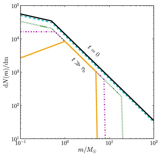
Schematic of the changes in the MF in a N = 105 cluster due to stellar evolution and the preferential ejection of low-mass stars, based upon figs 1 and 2 of Lamers et al. (2013). The lines represent the shape of the MF at different times, from cluster formation (t = 0) to late evolution (t ≫ τb). The initial MF (black, solid) is given by a Kroupa (2001) MF between 0.1 and 100 M⊙. Early evolution (for t < τe) removes stars uniformly across the MF, without changing its shape. At τe (cyan, dashed), the highest mass stars begin to explode as supernovae, removing them from the cluster. Meanwhile stars are ejected from the entire MF until τb (green, dotted), whereafter we assume stars are preferentially ejected from the low-mass end of the MF. The next line (magenta, dot–dashed) shows the progression of both stellar evolution and the preferential ejection of low-mass stars simultaneously, until late times when N ≪ N0 (orange, solid). For these last lines, the slope of the MF at the low-mass end inverts due to the absence of (remaining) low-mass stars. It is apparent that the two effects affect opposite ends of the MF.
![Comparison of our analytic fit for τe (as a function of mup; see equation 6) to the main-sequence lifetimes of stars predicted by the models of Hurley et al. (2000). Note that by using our definition of τe, we are able to invert the function and hence recover mup(t) as a function of t. Since the assumed mass of neutron stars and white dwarfs is m ≃ 1.2 M⊙ and we make the assumption that a fraction of these are retained by the cluster, τe is infinite for m ≤ 1.2 M⊙ [i.e. we do not expect to find mup(t) ≥ 1.2 M⊙ at any time]. For this figure, we predict τe for a range of stellar masses 1.2 M⊙ ≤ m ≤ 100 M⊙, with an expected main-sequence lifetime of a 100 M⊙ star τe = 3.3 Myr, and use a value a = 2.7. We note, however, that emacss assumes a Kroupa (2001) IMF with mlow = 0.1 M⊙, and a value of mup(t) that defines τe as shown by this plot.](https://oup.silverchair-cdn.com/oup/backfile/Content_public/Journal/mnras/442/2/10.1093/mnras/stu899/2/m_stu899fig3.jpeg?Expires=1749881606&Signature=3G0t~xVritXey3JD3gYVrwELIxKkHwAd714vvXuA2TaCd8s5YuBKnSQbv-SI2r9xe~k5hhr6-hzMGNCvgnnBZI8W5tadMbyfAvSJh6g1~ZnsVwAxtyuX72TQ1~OX9KGYqjS~9G8d6tHjrAAcXUZ4GQ5JgwFyfX-ZJJusmmc2tXNlWJiKrTM2g2N-xZpmcKp8H9KrB1p5pRLFOe2i4o3wQgTxrighTTEIEjiVD3qSqZZdPmW2rAQeN2MvnSlUYh8xJFU-e1Ci8xYFmSMe-TpI6v~XCwvUhEic2QnfViAYcl1prIfZm~zqSq5p3zr-PU1J6N2dx3jrVLY3MrPnDlPqTg__&Key-Pair-Id=APKAIE5G5CRDK6RD3PGA)
Comparison of our analytic fit for τe (as a function of mup; see equation 6) to the main-sequence lifetimes of stars predicted by the models of Hurley et al. (2000). Note that by using our definition of τe, we are able to invert the function and hence recover mup(t) as a function of t. Since the assumed mass of neutron stars and white dwarfs is m ≃ 1.2 M⊙ and we make the assumption that a fraction of these are retained by the cluster, τe is infinite for m ≤ 1.2 M⊙ [i.e. we do not expect to find mup(t) ≥ 1.2 M⊙ at any time]. For this figure, we predict τe for a range of stellar masses 1.2 M⊙ ≤ m ≤ 100 M⊙, with an expected main-sequence lifetime of a 100 M⊙ star τe = 3.3 Myr, and use a value a = 2.7. We note, however, that emacss assumes a Kroupa (2001) IMF with mlow = 0.1 M⊙, and a value of mup(t) that defines τe as shown by this plot.
Both this section and Section 4.2.1 consider very simple descriptions for the evolution of the MF, in which the only measurable quantity is |$\bar{m}$|. Although more complete descriptions for the MF exist (e.g. the ‘differential mass function’ of Lamers et al. 2013), in order to retain the clarity of this work we refrain from using more complex descriptions.
4.3 Energy of escapers during unbalanced evolution
Stars escape from SCs on account of either internal processes (i.e. stars are lost from isolated clusters; Baumgardt et al. 2002), or, for clusters tidally limited by the presence of a galaxy, interaction with the tidal field (Fukushige & Heggie 2000). The escape of stars causes SC mass to decrease over time, which will consequently increase the gravitational binding energy (i.e. escapers constitute a positive contribution E). As stars escape via the Lagrange points with v ≃ 0, the energy change due to each escaper will depend only on the potential experienced by the star when it escapes, i.e. |$\dot{E} = m_{\rm esc}\phi _{\rm e} \dot{N}$| and ϕe = −GM/rJ is the potential at the Jacobi surface rJ.
4.4 Post-collapse (balanced) evolution
All clusters will eventually reach a ‘balanced’ state (Gieles et al. 2011) at the time that a regulatory mechanism is formed in the core (roughly at core collapse; Hurley & Shara 2012). In this state, energy changes within the core (binary action, interactions with stellar- or intermediate-mass black holes and ongoing stellar evolution; Spitzer & Hart 1971; Heggie 1975; Gieles et al. 2010; Breen & Heggie 2013) are regulated by the behaviour of the cluster as a whole and not by local processes (Hénon 1961), leading to a radial flux of energy in the cluster that, for single-mass clusters, is constant per unit of relaxation time (|$\dot{E}\tau _{\rm rh}/E=\,$|constant).
For multi-mass models we find that this energy flux depends on time, such that |$\dot{E}\tau _{\rm rh}/E= f(t)$| (a monotonically decreasing function of time). This decrease emanates from the decreasing ratio between mup(t) and mlow, which decreases the rate at which energy can be transported through a cluster by relaxation. We have previously accounted for this decreasing efficiency of relaxation by including a ψ term (equation 5) in the definition of |$\tau _{\rm rh}^{\prime }$|. Hence, for clusters with an evolving MF, we find that |$\dot{E}\tau _{\rm rh}^{\prime }/E=\,$|constant, and that the constant is once again given by ζ (see equation 12).
5 CHANGES IN CLUSTER PROPERTIES DURING UNBALANCED EVOLUTION
In Section 4, we examined the mechanisms through which the external energy of an SC changes. This change in energy is related by equation (2) to a number of cluster properties; the loss of stars (|$\dot{N}$|), a change in cluster half-mass radius (|$\dot{r}_{\rm h}$|), and a change in the energy form factor due to a changing density profile (|$\dot{\kappa }$|). We examine the evolution of each property in turn below (for unbalanced clusters).
5.1 Escape of stars
5.1.1 Relaxation-driven escape
In Paper I we developed a description for the dimensionless escape rate ξe using the works of Gieles & Baumgardt (2008) and Fukushige & Heggie (2000). From these works, we showed that |$\xi _{\rm e}\propto \mathcal {R}_{\rm hJ}^{3/2}(N/\ln \gamma _{\rm c}N)^{1/4}$| where |$\mathcal {R}_{\rm hJ}\equiv r_{\rm h}/r_{\rm J}$| and can be understood as a RV filling factor. This term implies that ξe will be higher if rh is larger compared to rJ. The second term [(N/ln γcN)1/4] reduces the rate of escape from low-N systems, and accounts for the ‘escape time effect’ in which escape is delayed due to the anisotropic geometry of the Jacobi surface (Baumgardt 2001).
In Paper II we introduce two additional terms, f and |$\mathcal {F}$|, to improve the description of ξe for the unbalanced regime. The first of these terms, f ≃ 0.3, accounts for the lower escape rate observed in N-body simulations for unbalanced SCs (Lamers et al. 2010, Paper II). The second term, |$\mathcal {F}$|, accounts for the progress of core collapse, and is defined in Paper II as |$\mathcal {F}= \mathcal {R}_{\rm ch}/\mathcal {R}_{\rm ch}^{\rm min}$|.
The values of N1, |$\mathcal {R}_1$| and z determined in Paper I are true for clusters of single-mass stars, but do not necessarily remain useful for multi-mass clusters. We therefore redefine these quantities for clusters with MFs through comparison against N-body simulations, and note that they remain constant throughout both unbalanced and balanced evolution.
5.1.2 Induced escape
Although equation (32) is by construction somewhat approximate, this is unlikely to affect the application of emacss to realistic globular clusters (e.g. Harris 1996, 2010 version). This is because the majority of clusters are likely to have formed RV under-filling (see Alexander & Gieles 2013; Ernst & Just 2013), where find ≃ 0. Consequently, this term will only be applicable to a minority of clusters.
5.2 Change of the density profile
The original emacss (Paper I) correctly reproduces the evolution of virial radius (rv), but ignores the variation of κ and therefore assumes that rh/rv = 1 throughout SC evolution. During the balanced phase, this is a reasonable assumption as the variation in κ is mild. During unbalanced evolution however, the variation of κ is significant since the central density changes extremely quickly as the core undergoes collapse (Giersz & Heggie 1996). This is discussed in depth in Paper II for clusters of single-mass stars, where it is shown that κ varies on account of a varying |$\mathcal {R}_{\rm ch}$|.
In Paper II, κ is shown to be adequately described by an error function of |$\mathcal {R}_{\rm ch}$| which varies between κ0 ≃ 0.2 at birth (the initial value of κ for a W0 = 5 King 1966, model), and κ1 ≃ 0.24 at late times (roughly the value of κ for the typical density profile measured during the balanced evolution following core collapse). This evolution of κ corresponds to the change in energy form factor for a cluster during the ‘gravothermal catastrophe’ (Lynden-Bell & Eggleton 1980), which is generally only experienced by clusters of single-mass stars. For clusters containing (or containing stars sufficiently massive to evolve into) black holes, the core-radius is also linked to the retention of black holes, which is a random effect and hence cannot be reliably modelled. The evolution of half-mass radius, however, does not depend upon the energy sources in the core, and thus can be modelled without knowledge of the core radius and black hole retention (Breen & Heggie 2013; Lützgendorf et al. 2013).
5.3 Evolution of the half-mass radius
6 CHANGES IN CLUSTER PROPERTIES DURING BALANCED EVOLUTION
Once an SC has reached a state of balanced evolution, the energy production is controlled by the whole cluster as opposed to the energy-generating core. In this state, the energy change per |$\tau _{\rm rh}^{\prime }$| is given by a single quantity (ζ), and does not depend on any of the mechanisms outlined in Sections 4.1, 4.2 and 4.3. Like in the unbalanced phase, the change of energy leads to several dynamical effects, although unlike in the unbalanced phase the density profile does not significantly change. We are left therefore with three evolutionary effects: the escape of stars, expansion or contraction of the half-mass radius, and the changing mean mass of stars.
6.1 Escape of stars
6.2 Changing mean mass of stars
Although the change in |$\bar{m}$| due to stellar evolution no longer defines energy production in the balanced phase, stellar evolution will continue to reduce the mass of the highest mass stars, and escaping stars will typically continue to deplete the low-mass end of the MF. We find therefore that once again γ = γs + γe in balanced evolution, although this is no longer related to ϵ.
6.3 Expansion and contraction
7 COMBINED OPERATION OF EMACSS
Following the philosophy outlined in Papers I and II, we encapsulate the entire evolution of clusters in terms of several key quantities. Energy changes are categorized by a single parameter, ϵ, which takes one of three forms at each stage of evolution: unbalanced evolution before and after τe, and balanced evolution. The equations used to calculate the changing energy in each of these regimes are summarized in Table 1, while the energy change due to the impact of these three processes is illustrated in Fig. 4.
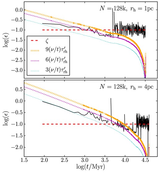
Evolution of ϵ as a function of time for the rh = 1 pc and rh = 4 pc, N = 128k SCs. In each plot, the (black) solid line is calculated using equation (7) from N-body data. The (red) dashed line is ϵ = 0.1 (i.e. balanced evolution), while the three dotted lines are the energy changes due to stellar evolution for different (constant) mass segregation factors. Core collapse is evident as a jump in ϵ. The N-body data cross several of the dotted lines due to increasing mass segregation. We do not see a period without internal energy changes as the N-body simulations do not have sufficient resolution in the first ≃100 Myr for this to be apparent.
The definitions of ϵ during the three phases of cluster evolution. The quantity nc defines a number of elapsed modified relaxation times at which balanced evolution begins (which occurs when t = τb), and is determined by comparison with N-body simulations. The remaining quantities use are defined in Tables 2 and 3.
| t < τe | |${\epsilon =\displaystyle \frac{1}{\kappa }\frac{m_{\rm esc}}{\bar{m}}\frac{r_{\rm h}}{r_{\rm J}}\xi }$| | Unless balance begins before the supernovae of the most massive stars, the energy of an SC does not change by any internal processes in the first few Myr (depending on the upper limit of the MF). It may, however, change due to external processes, such as the direct removal of stars by an external tidal field. We include this contribution, although note that it is negligible for clusters that are initially sufficiently compact. |
| τe < t < τb | |${\epsilon =\displaystyle \frac{1}{\kappa }\frac{m_{\rm esc}}{\bar{m}}\frac{r_{\rm h}}{r_{\rm J}}\xi +\mathcal {M}\gamma _{\rm s}}$| | Unbalanced evolution, described in Section 4.2.1. The first term accounts for the energy change due to stars escaping directly by dynamical processes. Meanwhile, the second term represents the decrease in |$\bar{m}$| and hence increase in cluster energy through stellar evolution (which are related via equation 2). The extent of this energy change depends on whether the mass loss occurs centrally or uniformly (i.e. depends upon the degree of mass segregation, |$\mathcal {M}$|). |
| t > τb | |${\epsilon =\displaystyle \zeta }$| | Balanced evolution, defined in Paper I; |$\dot{E}/E\tau _{\rm rh}= {\rm const}$| for clusters of single-mass stars, but is time dependent for multi-mass clusters due to the decreasing range of the MF. In this paper, ϵ is related to |$\tau _{\rm rh}^{\prime }$| such that |$\dot{E}/E\tau _{\rm rh}^{\prime } = \zeta$|, and the time dependence due to an evolving MF is incorporated into our definition of |$\tau _{\rm rh}^{\prime }$|. This state continues until very near the final dissolution of the cluster when N ≃ 200 and balanced evolution breaks down because τrh becomes comparable to the crossing time. |
Based on Fig. 4, we find that ζ = 0.1 (as in Paper II) fits our data when ψ1 = 8.0 and ψ0 = 1.6. This implies that even during the late stages of balanced evolution, the conduction of energy is more efficient for an SC with an MF than an equal-mass cluster. as previously suggested (e.g. Lamers et al. 2013), this result is consistent with clusters’ MFs evolving towards a narrow (delta function like) shape similar to that of single-mass clusters. However, such clusters retain some range of MF for their entire lifespan. We consequently adopt these values, such that ψ1 = 8.0, ψ0 = 1.6 and ζ = 0.1 hereafter.
The transition between the second and third stages of energy production (the start of balanced evolution) occurs after a time τb whose physical value is not known at t = 0. The transition between the first and second stages occurs when the highest mass stars present explode as supernova (at τe = 3.3 Myr for mup = 100 M⊙ stars), unless the SC is undergoing balanced evolution before this time.
Whereas the energy changes in an SC are summarized in Table 1, the consequences of changing the energy of an SC are summarized in Table 2. We also define the dimensionless parameters involved in SC evolution, and the ancillary equations used by our model. Finally, Table 3 summaries the key scaling factors and constants present. When known, the values of these parameters are quoted from literature.
The main equations used by emacss. The first section defines the differential equations that calculate the evolution of the measurable quantities (e.g. N, |$\bar{m}$|, and rh). The second section defines the dimensionless factors used in these equations, while the third section defines additional factors used by the preceding equations in each time-step. Additional parameters derived from the variables modelled by emacss are defined in the final section.
| Output properties evolved by emacss | |
| |$\dot{E} = \frac{\epsilon |E|}{\tau _{\rm rh}^{\prime }}$| | Rate of change of the external energy of stars. Virial equilibrium is assumed throughout, such that E = U/2. |
| |$\dot{N} = -\frac{\xi N}{\tau _{\rm rh}^{\prime }}$| | Rate of change of the total number of bound stars. |
| |$\dot{r}_{\rm h}= \frac{\mu r_{\rm h}}{\tau _{\rm rh}^{\prime }}$| | Rate of change of the half-mass radius. |
| |$\dot{\bar{m}} = \frac{\gamma \bar{m}}{\tau _{\rm rh}^{\prime }}$| | Rate of change of the mean mass of bound stars. |
| |$\dot{\kappa } = \frac{\lambda \kappa }{\tau _{\rm rh}^{\prime }}$| | Rate of change of the energy form factor, related to the density profile. |
| |$\dot{\mathcal {M}}= \mathcal {M}\frac{\mathcal {M}_1 - \mathcal {M}}{\tau _{\rm rh}^{\prime }}$| | Rate of change of the concentration parameter for evolving stars. Defined so as to express the efficiency of the adiabatic expansion caused by stellar evolution [i.e. |$\dot{E}/|E| = -\mathcal {M}\dot{\bar{m}}/{\bar{m}}$|, and so |$\dot{r}_{\rm h}/r_{\rm h}= -(\mathcal {M}-2)\dot{\bar{m}}/{\bar{m}}$|]. |
| |${\dot{\bar{m}}_{\rm s}}= \frac{\gamma _{\rm s}\bar{m}}{\tau _{\rm rh}^{\prime }}$| | Rate of change of the mean mass of stars due only to the in situ mass loss caused by stellar evolution. If escaping stars have no preferential mass (e.g. all masses of stars are ejected), |$\bar{m}\equiv \bar{m}_{\rm s}$|. |
| Dimensionless (differential) parameters | |
| ξ = ξe + ξi | Dimensionless escape rate per |$\tau _{\rm rh}^{\prime }$| due to both direct and induced mechanisms. |
| |$\xi _{\rm e}= \mathcal {F}\xi _0(1-\mathcal {P})+\left[f+(1-f)\mathcal {F}\right]\frac{3}{5}\zeta \mathcal {P}$| | Direct relaxation driven escape rate. The first term comes from internal effects (Baumgardt et al. 2002) and the second from mass loss due to a tidal field (Paper I and references therein). |
| ξi = findγs | Dynamical escape rate per |$\tau _{\rm rh}^{\prime }$| induced by stellar evolution. |
| μ = ϵ − 2ξ + 2γ + λ | Dimensionless change of rh per |$\tau _{\rm rh}^{\prime }$| due to dynamical and stellar evolution. Responds so as to maintain the balance of energy (i.e. by conservation of energy). |
| γ = γs + γe | Dimensionless change in |$\bar{m}$| due to both stellar evolution and the preferential ejection of low-mass stars. |
| |$\gamma _{\rm s}= -\frac{\nu \tau _{\rm rh}^{\prime }}{t}\frac{\bar{m}_{\rm s}}{\bar{m}}$| | Dimensionless change in |$\bar{m}$| due to stellar evolution. |
| |$\gamma _{\rm e}= \left[1-\frac{m_{\rm esc}}{\bar{m}}\right]\mathcal {S}\mathcal {U}\xi$| | Dimensionless change in |$\bar{m}$| due to the preferential ejection of low-mass stars. |
| $\lambda = \left\{\begin{matrix}
0, & n\,{<}\,n_{c}/2,\\
(\kappa _{1}-\kappa )\left ( \frac{2n}{n_{c}}-1 \right ), & {\rm otherwise,}
\end{matrix}\right.$ | Dimensionless change in the energy form factor, most significant just prior to core collapse (e.g. see Paper II). In Paper II an alternative definition is used to represent the gravothermal catastrophe. However, since SCs with MFs do not undergo the gravothermal catastrophe, we use an approximate form in this study. |
| Variable factors | |
| |$\mathcal {P}= \left(\frac{\mathcal {R}_{\rm hJ}}{\mathcal {R}_{1}}\right)^z\left[\frac{N\log (\gamma _{\rm c}N_1)}{N_1\log (\gamma _{\rm c}N)}\right]^{1-x}$| | Function parametrising the rate of escape due to a tidal field (Paper I). |
| $\mathcal {F}= \left\lbrace \begin{array}{@{}ll@{}}
0, & \,\,\, n {<} n_{\rm c}/2,\\
\left(\frac{2n}{n_{\rm c}}-1\right), & \,\,\, n_{\rm c}/2 \le n \le n_{\rm c},\\
1, & \,\,\, n_{\rm c}{<} n, \end{array}\right.$ | Smoothing factor to connect the escape rate in unbalanced evolution to the escape rate in balanced evolution. In Paper II it was assumed |$\mathcal {F}= \mathcal {R}_{\rm ch}^{\rm min}/\mathcal {R}_{\rm ch}$|, although rc is not available for this case. We therefore use an approximation that behaves in an equivalent manner. |
| |$\tau _{\rm e}(m) = \tau _{\rm e}(m_{\rm up})\left[1+\frac{\ln (m/m_{\rm up})}{ \ln (m_{\rm up}/m_{\rm up}^{\infty })}\right]^{a}$| | Time before the supernova of the most massive star, as a function of the upper limit of the MF (mup). Based on the analytic description of Hurley et al. (2000): see Fig. 3. This function can be inverted to give mup(t) as a function of t. |
| |$\mathcal {S}= [(\mathcal {M}-3)/(\mathcal {M}_1-3)]^q$| | Factor relating the mass segregation to the depletion of low-mass stars. |
| |$\mathcal {U}= (m_{\rm up}(t)-\bar{m})/(m_{\rm up}(t))$| | Factor to ensure |$\bar{m}{<} m_{\rm up}(t)$| at all times. |
| |$m_{\rm esc}= \mathcal {X}\left(\bar{m}-m_{\rm low}\right)+m_{\rm low}$| | (Average) mass of an escaping star. |
| ${f}_{\rm ind}= \left\lbrace \begin{array}{@{}ll@{}}
\mathcal {Y}\left(\mathcal {R}_{\rm hJ}-\mathcal {R}_{1}\right)^b, & \mathcal {R}_{\rm hJ}> \mathcal {R}_{1}, \\
0, & {\rm otherwise.} \end{array}\right.$ | Approximation for the relationship between induced escape to mass loss through stellar evolution (see Lamers et al. 2010). |
| $\psi (t) = \left\lbrace \begin{array}{@{}ll@{}}
\psi _{\rm 1}, & \,\,\, t \le \tau _{\rm e}, \\
(\psi _{\rm 1}-\psi _{\rm 0})\left[\frac{t}{\tau _{\rm e}(m_{\rm up})}\right]^{y}+\psi _{\rm 0}, & \,\,\, t {>} \tau _{\rm e}.
\end{array}\right.$ | Modification to the standard definition of τrh, adjusting to account for the presence of a MF. Approximately represents |$\psi = \overline{m^{\beta }}/\overline{m}^{\beta }$|: see (Spitzer & Hart 1971). |
| Derived cluster properties | |
| |$\tau _{\rm rh}= 0.138\frac{\left(Nr_{\rm h}^3\right)^{1/2}}{\sqrt{G\bar{m}}\log (\gamma _{\rm c}N)}$| | Mean relaxation time of stars within the half-mass radius (Spitzer 1987). |
| |$\tau _{\rm rh}^{\prime } = \frac{\tau _{\rm rh}}{\psi (t)}$| | Modified relaxation time of stars within the half-mass radius, adjusted to consider the presence of a MF. See (Spitzer & Hart 1971). |
| |$n= \int ^{t}_0 \frac{{\rm d}t}{\tau _{\rm rh}^{\prime }}$| | Number of modified relaxation times that have elapsed at time t. |
| |$r_{\rm J}= R_{\rm G}\left[\frac{N\bar{m}}{2M_{\rm G}(<R_{\rm G})}\right]^{\frac{1}{3}}$| | Jacobi (tidal) radius for an isothermal galaxy halo. For a point-mass galaxy the factor of 2 in the denominator is replaced by a factor of 3. The mass contained within the galactocentric (orbital) radius is defined by MG(<RG). |
Definitions of constants used by emacss to define cluster evolution. The values of these constants are taken from literature where possible, or calibrated against N-body data when not.
| ζ = | Fractional conduction of energy for clusters with globular cluster like MFs. In Paper I we find (for clusters of single-mass stars) ζ0 = 0.1. For this study, we retain this definition although note that the conduction of energy is time dependent (owing to our redefinition of |$\tau _{\rm rh}^{\prime }$|). |
| y = | Power-law exponent used to express the width of the stellar MF as a function time. Gieles et al. (2010) show that a good approximation to the theory of Spitzer & Hart (1971) is provided by y = −0.3. |
| γc = | Argument of the Coulomb Logarithm. From Giersz & Heggie (1996), γc = 0.11 for single-mass clusters and γc = 0.02 for multi-mass clusters. |
| ξ0 = | Dimensionless escape rate of an isolated cluster. From Paper I (for clusters of single-mass stars), ξ0 = 0.0141. |
| |$\mathcal {R}_{1}$| = | Ratio of rh to rJ. From Hénon (1961) for RV filling clusters of single-mass stars, |$\mathcal {R}_{1}= 0.145$|. For multi-mass clusters, we measure from Fig. 5a scaling relationship between |$\mathcal {R}_{1}$| and N1, and show that |$\mathcal {R}_{1}= 0.22$| lies upon the track of all our simulations where N1 = 1000. |
| z = | Power-law exponent used to express the scaling of ξe with rh around |$\mathcal {R}_{1}$|, see Gieles & Baumgardt (2008). It is shown in Paper I that z = 1.61 for clusters of equal-mass stars. |
| x = | Power-law exponent used to express the scaling on ξe with N due to the escape time effect. From Baumgardt (2001), x = 0.75. |
| |$\mathcal {X}$| = | Factor determining the mean (average) mass of ejected stars. If |$\mathcal {X}= 0$|, mesc = mlow, while if |$\mathcal {X}= 1$|, |$m_{\rm esc}= \bar{m}$| and |$0 \le \mathcal {X}\le 1$|. |
| N1 = | Scaling factor, defining an ideal cluster for which the ratio |$\mathcal {R}_{\rm hJ}=\mathcal {R}_{1}$|. From Paper II (for clusters of single-mass stars), N1 ≃ 15 000. For multi-mass clusters, we measure from Fig. 5a scaling relationship between |$\mathcal {R}_{1}$| and N1, and show that N1 = 1000 lies upon the track of all our simulations where |$\mathcal {R}_{1}= 0.22$|. |
| ν = | Power-law exponent used to express the change of |$\bar{m}$| with respect to time due to stellar evolution (typically) at the high-mass end of the MF. From Gieles et al. (2010) for a Kroupa (2001) IMF, ν = 0.07. |
| τe = | Time before the start of stellar evolution (i.e. main-sequence lifetime of the most massive star present). From stellar evolution models with a maximum star mass of 100 M⊙, τe = 3.3 Myr. |
| a = | Power defining the relationship between main-sequence lifetime and stellar mass. Fit in Fig. 3 against the stellar evolution theory of Hurley et al. (2000), where it is shown a = −2.7 provides a satisfactory fit. |
| nc = | Number of modified relaxation times (|$\tau _{\rm rh}^{\prime }$|) that elapse prior to the start of balanced evolution. We also define balanced evolution as beginning at time τb, although this cannot be calculated at t = 0. |
| |$\mathcal {M}_{\rm 1}$| = | Scaling factor defining the efficiency of energy production in a fully mass segregated cluster. |
| f = | Factor by which the escape rate is reduced in unbalanced evolution. From Paper II, f = 0.3. |
| κ0 = | Initial energy form factor, κ0 ≃ 0.2 for a King (1966) or Plummer (1911) model. |
| κ1 = | Energy form factor during balanced evolution. From Paper II, κ1 ≃ 0.24. |
| ψ0 = | Modification factor for |$\tau^{\prime}_{\rm rh}$| at late times (i.e. with negligible range of remaining MF). Measured in Section 7 to be ψ0 = 1.6. |
| ψ1 = | Modification factor for |$\tau^{\prime}_{\rm rh}$| at early times (t = 0). Measured in Section 7 to be ψ1 = 8.0. |
| q = | Scaling index that relates the degree of mass segregation to the degree of low-mass depletion. |
| |$\mathcal {Y}$| = | Factor defining the |$\mathcal {R}_{\rm hJ}$| dependence of ξi. |
| b = | Power scaling the induced mass loss to RV filling factor, determined by comparison against N-body data. |
There are several new parameters for which literature values are not available. Specifically, for a cluster in isolation the maximum efficiency factor for energy production by stellar evolution, |$\mathcal {M}_{\rm 1}$|, is not known, and the number of scaled |$\tau _{\rm rh}^{\prime }$| that pass before balanced evolution begins (nc) is not defined. Furthermore, we use N-body data to determine an approximate value for the excess mass of a typical ejected star (|$\mathcal {X}$|), and the index defining the degree to which mass segregation affects low-mass depletion (q).
Because the direct escape rate from multi-mass clusters is not necessarily the same as for clusters of single-mass stars, we need to redefine N1, z and |$\mathcal {R}_{1}$|. The definitions of N1 and |$\mathcal {R}_{1}$| are highly (though not totally) degenerate (see Paper I, Appendix A), and define coordinates in an |$(N,\mathcal {R}_{\rm hJ})$| space through which (contracting and RV filling) clusters will eventually evolve. The relationship between these parameters is illustrated in Fig. 5, from which we choose a pair of parameters |$(N_1, \mathcal {R}_{1}) = (1000,0.22)$| for scaling. We have not used the original definition |$\mathcal {R}_{1}= 0.145$| from Hénon (1961), Paper I and II since this value is significantly lower than the |$\mathcal {R}_{\rm hJ}$| values measured in any of our new N-body simulations. While it would be possible to extrapolate to a much higher N1 where |$\mathcal {R}_{\rm hJ}=0.145$|, the corresponding N1 is well above our range of N under test and would significantly change ξe due to the N dependence of the Coulomb logarithm.
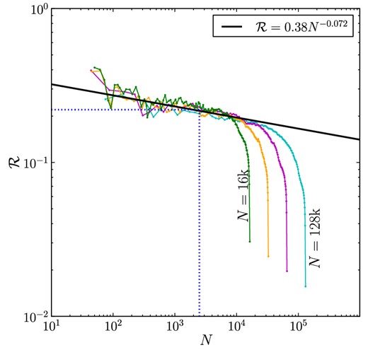
Evolution of |$\mathcal {R}_{\rm hJ}$| as a function of N for N-body simulations. In this figure, the evolution of time goes from right to left. The simulations have N = 16, 32, 64 and 128k stars as labelled, and begin with rh = 1 pc. All the clusters begin their evolution with expansion, but eventually evolve towards the same track in the |$N-\mathcal {R}_{\rm hJ}$| space once RV filling. The (black) solid line is a single-power-law fit, while the (blue) dotted lines demonstrate a reference pair of N and |$\mathcal {R}_{\rm hJ}$| that lie upon the track of common evolution, well within the region in which all clusters are RV filling. We let this pair be N1 and |$\mathcal {R}_{1}$|, and therefore choose N1 = 1000 and |$\mathcal {R}_{1}= 0.22$| for multi-mass clusters with stellar evolution.
Finally, our definition of the efficiency of induced mass loss is new and therefore has not been previously measured. To this end, we define values for |$\mathcal {Y}$| and b by comparison against N-body simulations of RV filling clusters. The parameters that are optimized by comparison against N-body data in Section 8 are |$\mathcal {M}_{\rm 1}$|, nc, z, |$\mathcal {X}$|, |$\mathcal {Y}$|, q and b.
7.1 The model (emacss)
Using the quantities, properties, and equations defined in Tables 1 –3, we extend the theoretical framework upon which emacss is based. As in Papers I and II, we solve the various differential equations for incremental time-steps using Runge–Kutta numerical integration.
In Paper I, it is trivial to calculate an appropriate time-step size for the Runge–Kutta scheme, since clusters of single-mass stars have only one time-scale (relaxation) defining their evolution. Hence, the step-size is always set to be 0.1τrh. In Paper II, however, a second time-scale (the core relaxation time-scale) becomes relevant, and becomes significantly shorter than 0.1τrh (and hence paramount for accuracy) for the runaway stages of core collapse. To compensate for this, in Paper II a combined time-step is used including both τrh and the core relaxation time. For multi-mass clusters there are again two distinct time-scales: relaxation, and stellar evolution (which has a time-scale ≃ t; see equation 15). A time-step optimized for stellar evolution will be shorter than relaxation when t is small, but will quickly grow to become much larger than τrh.
The sequence of calculations performed by emacss is as follows.
An (estimated) duration of the next time-step is computed from previous time-step duration and accuracy.
The change in energy during the upcoming time-step, ϵ, is computed by the formulae in Table 1, while the dimensionless constants (|$\xi _{\rm e}, \xi _{\rm i}, \mu , \gamma _{\rm s}, \gamma _{\rm e}, \mathcal {M}_1, \lambda$|) and characteristic properties (|$\tau _{\rm rh}, \tau _{\rm rh}^{\prime }, r_{\rm J}, {f}_{\rm ind}$|) are determined.
A fifth order Runge–Kutta integration step is applied to equations (7) through (11), updating parameters as required. The new state of the cluster (e.g. N, |$\bar{m}$|, rh, κ) is found.
The truncation error due to the approximations used by the numerical integrator is examined. If it is large (>10−4 per cent), the code repeats from step (i) using a smaller time-step. If it is acceptable, or if further reduction would cause an overly small time-step (see equation 37), the step is completed and the code progresses. The values are chosen such that a cluster's lifecycle is described by ≃1000 time-steps, which is fewer than previous versions on account of the efficiency increase offered by the adaptive Runge–Kutta scheme.
Specified values are output.
Steps (i) through (v) are repeated until N ≤ 200, which is consistent with Papers I and II (N = 200) and represents the ‘breakdown’ of balanced evolution due to stochastic effects.
For the sake of simplicity, the working of emacss is performed in N-body units (i.e. |$G =N\bar{m}= -4E = r_{\rm v}= 1$|; Heggie & Mathieu 1986), although conversion to physical units (Myr, M⊙, pc) is trivial. In order to facilitate easy comparison to ‘real’ SCs, this conversion is (by default) performed at output.
8 GENERAL RESULTS
As emacss is intended to model SCs evolving with a range of initial conditions and tidal environments, we benchmark the efficacy of our prescription against the N-body data base outlined in Section 2. We first optimize our prescription for simple (isolated) models, before increasing the complexity through the addition of a tidal field. For isolated clusters we have just two undefined parameters (|$\mathcal {M}_{\rm 1}$| and τb), while there are five additional parameters for tidally limited clusters (z, |$\mathcal {X}$|, |$\mathcal {Y}$|, b and q). We first fit |$\mathcal {M}_{\rm 1}$| and τb for our simulations of isolated clusters in Section 8.1, before fitting z, |$\mathcal {X}$|, |$\mathcal {Y}$|, b and q for our tidally limited simulations in Section 8.2. We also show some additional comparisons against clusters in additional tidal fields and on eccentric orbits in Appendix A. Throughout, we use |$(N_1, \mathcal {R}_{1}) = (1000,0.22)$| as demonstrated in Section 7.
8.1 Isolated clusters
Fig. 6 shows the evolution of several parameters (N, rh, |$\bar{m}$|, E) from N-body simulations of isolated SCs (see Section 2). Over-plotted are the equivalent tracks predicted by emacss for clusters with the same initial conditions, with our best-fitting parameters of |$\mathcal {M}_{\rm 1}= 4$| and nc = 12.5.
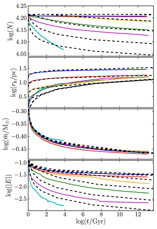
Comparison of N (top), rh, |$\bar{m}$|, and E (bottom) as a function of t for the model described in Sections 4, 5 and 6 to N-body data for isolated clusters from Section 2. The simulations are chosen such that the range of τrh0 is logarithmically spaced between 0.03 and 3 Gyr, with the topmost (blue) track being that of the τrh0 = 3 Gyr simulation and the lowest (cyan) being the τrh0 = 0.03 Gyr simulation.
The evolution of |$\bar{m}$| in the third panel is well described by a single-power law for isolated clusters, using the same ν = 0.07 as measured by previous studies (e.g. Gieles et al. 2010). This is consistent with the loss of mass due to stellar evolution, which is (for isolated clusters) the predominant cause of mass loss. Further to this, an expansion of rh such that |$\dot{r}_{\rm h}/r_{\rm h}= -(\mathcal {M}-2){\dot{\bar{m}}_{\rm s}}/\bar{m}$| is shown to provide an adequate description of the rh evolution, implying that |$\mathcal {M}$| evolves in a similar manner to that suggested in Section 5, and that energy evolves such that |$\dot{E}/|E| = -\mathcal {M}{\dot{\bar{m}}_{\rm s}}/\bar{m}$|. The start of balanced evolution is evident as an upturn in the rh evolution in both N-body data and the predictions of emacss, suggesting that our value nc = 12.5 is appropriate for these clusters.
We find that the escape rate from isolated clusters with stellar evolution is somewhat over-predicted if we retain the description of escape from Paper I (see equation 27), whereby (in isolated clusters) the fraction of escapers ξ0 = 0.0142 per |$\tau _{\rm rh}^{\prime }$|. The over-prediction of ξ is accounted for by our use of |$\tau _{\rm rh}^{\prime }$| which (at early times) is a factor of ∼8 smaller than τrh. We find this over-prediction is reduced if we redefine ξ0 = 0.0075. The value |$\mathcal {M}_{\rm 1}= 4$| chosen is somewhat lower than expected. However, there is some data (specifically, the rh increase of the short initial τrh clusters) to suggest that the mass segregation is higher than |$\mathcal {M}_{\rm 1}= 4$| within the first ≃1 Gyr, which is evidenced by the under-predicted expansion and energy increase produced by emacss. A higher |$\mathcal {M}_{\rm 1}$| results in excessive expansion of long τrh clusters at times ≳10 Gyr. This suggests that the mass segregation is more severe than |$\mathcal {M}_{\rm 1}= 4$| when high-mass stars are still present, although the effect reduces as high-mass stars evolve. The value obtained, |$\mathcal {M}_{\rm 1}= 4$|, therefore represents a compromise value. Despite this, rh is reproduced to within a factor of 2, suggesting a good qualitative description for the evolution of isolated clusters is obtained by our prescription, and note anyway that the numerical discrepancy is acceptable since realistic clusters do not evolve in a completely isolated state.
8.2 Clusters in tidal fields
Figs 7 –9 show the evolution of all parameters for the N-body simulations of SCs in tidal fields at RG = 8.5 kpc. Our remaining simulations – those of initially RV filling clusters at RG = 2.8 kpc or RG = 15 kpc, and those on eccentric orbits – are additionally shown in Appendix A. Once again, in all cases we have over-plotted the results of emacss using the best-fitting z, |$\mathcal {X}$|, |$\mathcal {Y}$|, b and q, while we use the |$\mathcal {M}=4$| and nc = 12.5 defined in Section 8.1. For these clusters, emacss provides a reasonable estimation of the properties of our N-body simulations, and exhibits similar (qualitative) features throughout.

Comparison of the emacss model described in Sections 4–6 to N-body data for a series of N-body simulations of clusters in tidal fields (approximated as isothermal haloes with VG = 220 km s−1 and RG = 8.5 kpc). The left column plots N, rh, |$\bar{m}$|, E, |$\mathcal {R}_{\rm hJ}$| and κ as a function of time, while the right column plots the same properties as a function of log (N). The initial conditions of the N-body simulations are described in Section 2, with N0 = 128 k (cyan track; longest surviving), N0 = 64 k (magenta), N0 = 32 k (orange), N0 = 16 k (green; shortest surviving) stars. The clusters are allowed to evolve until their eventual dissolution. For these SCs, rh0 = 1 pc.
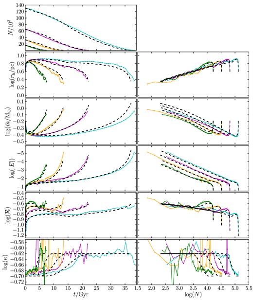
As Fig. 7, but with simulated clusters of larger initial radii. For these clusters, rh0 = 4 pc.

We find optimal values for our parameters to be z = 2.0, |$\mathcal {X}= 0.55$|, |$\mathcal {Y}=90$|, b = 1.35 and q = 2. In this case, z is somewhat higher than for the case of single-mass mass clusters, which may be caused by the mass segregation of the different stellar species. Because of mass segregation, low-mass species will form the majority of the SC halo, which (for the same density profile) will lead to increased numbers of stars in the outermost orbits. Consequently, the escape rate ξe is more sensitive to |$\mathcal {R}_{\rm hJ}$|, as suggested by a higher value of z. This theory is also supported by the value of |$\mathcal {X}= 0.55$|, since this implies that the escaping stars are (on average) mid-way between |$\bar{m}$| and mlow, and therefore have |$m {<} \bar{m}$|. If the majority of escapers are assumed to originate in the cluster halo, the value |$\mathcal {X}{<} 1$| confirms that the halo consists mainly of low-mass stars.
The power-law scaling for the rate of low-mass star depletion, q, is a free parameter, for which we find q = 2 fits well. This implies that the effects of mass segregation (represented by |$\mathcal {M}$|) are felt somewhat more strongly amongst the low-mass species (segregating outward into the halo) of the halo than the high-mass species (segregating inward towards the cluster core). If q is varied, we find that q ≪ 2 represents too weak a relationship between mass segregation and low-mass depletion (and too late an upturn in |$\bar{m}$|), while q ≫ 2 is too strong (with the upturn of |$\bar{m}$| occurring too early). The value q = 2 implies that mass segregation is slightly more strongly felt by low-mass species, perhaps as a consequence of high-mass stars starting to fall inward early and leaving a low-mass halo behind.
Since |$\mathcal {X}$| controls the ‘typical’ escaper mass and not (directly) a physical value, the value of |$\mathcal {X}$| is (reasonably) invariant throughout cluster evolution. This means that the mass of a (typical) escaping star will (correctly) increase as |$\bar{m}$| grows. This increase is also shown in the N-body data, and slows appropriately once |$\bar{m}$| approaches mup(t) (due to the increasing |$\mathcal {U}$| parameter). For the sake of simplicity, we retain a time invariant |$\mathcal {X}$|, and encompass the variation of mesc with respect to |$\bar{m}$| through |$\mathcal {U}$|. Further, we note that evolving stars are ipso facto assumed to lose all their mass, and hence that p = 0 (Section 4.2.2) throughout cluster evolution. Both these factors could be incorporated into a more exact model, and allowed to vary so as to offer an improved description of the evolution of cluster stars. A manner in which full variation of the MF could be built upon the work of Lamers et al. (2013), although for the sake of brevity we do not attempt this here, and caution that such models will be liable to significant stochastic effects.
Finally, the values found for |$\mathcal {Y}=90$| and b = 1.35 suggest that the induced mass loss increases quite rapidly once |$\mathcal {R}_{\rm hJ}> \mathcal {R}_{1}$|. This increased mass loss would imply that substantially overfilling clusters are unlikely to survive for a significant period of time. Instead, such RV overflowing clusters will lose their outermost stars very quickly, with the result that rh shrinks faster than rJ and the cluster returns to a filling- or under-filling state.
As in isolated clusters, the early unbalanced evolution of under-filling clusters is dominated by expansion, caused by the energy increase due to stellar evolution's mass loss. If SCs expand sufficiently to become RV filling before the end of the unbalanced phase, the rate of escape due to relaxation increases and the cluster will contract owing to a decreasing rJ. At the moment of core collapse however, ϵ instantaneously increases by a factor of ≃ 2–3, potentially leading to a secondary expansion (and later contraction) during balanced evolution. We find therefore that many of our RV under-filling clusters experience ‘double peaked’ radius evolution, depending on the range of the MF and the ratio |$\mathcal {R}$| at the time of core collapse.
For RV filling clusters, unbalanced evolution once again begins with an adiabatic expansion. However, in this case, the expansion very quickly causes the cluster to become over-filling, and hence always results in significant induced mass loss, meaning that the majority of the stars of a filling SC escape before core collapse. Furthermore, once a filling cluster reaches core collapse, it remains RV filling and hence continues to contract for the remainder of its life-cycle. For both filling- and under-filling SCs, the evolution of N is a smooth function of t since both ξe and ξi are functions of |$\mathcal {R}_{\rm hJ}$|, despite ϵ varying discontinuously.
Despite general success, there are several minor discrepancies between the N-body data and the emacss models for the various simulations. Some of these are random effects occurring in the N-body simulations (such as the fluctuations of post-collapse rh seen in the N-body simulations of Fig. 9 or the energy evolution of the 64k run in Fig. 8, which are simply the results of stochastic noise in the simulations). Others are accounted for by the various approximations made by our code – equation (27) approximates the geometry of the Jacobi surface and induced mass loss, which leads to the majority of the minor oscillation of N (or |$\mathcal {R}_{\rm hJ}$|, since rJ ∝ N1/3) in emacss when compared to N-body data. We also find that the |$\mathcal {R}_{\rm hJ}$| evolution shown in Fig. 9 is a somewhat less smooth curve for emacss than for the N-body data, which is most likely a consequence of the simplifications in the approximation for induced mass loss. Induced mass loss is likely to be a more complex process than appreciated by equations (31) and (32), as suggested in Lamers et al. (2010). Our most approximate overall quantity is the fitting function used for κ, which demonstrates the loosest fit to N-body data and perhaps exemplifies the weakest area of our code. This quantity is, however, of negligible importance for the overall properties we seek to model and which can be compared to observations.
The mean mass of stars in tidally limited N-body simulations shows an initial power-law decrease similar to that of isolated clusters. However, as predicted in Section 4.2.3, this eventually turns into an increasing |$\bar{m}$| due to the preferential ejection of low-mass stars. We find that emacss recovers this upturn to occur correctly for the majority of SC's lifetime.
9 CONCLUSIONS
We have enhanced the emacss prescription for SC evolution first presented in Papers I and II and originally based upon the work of Hénon (1961, 1965), and Gieles et al. (2011). Our enhancements incorporate the results of Lamers et al. (2010) (to describe the effect of stellar evolution upon escape) and Gieles et al. (2010) (to describe the effect of stellar evolution upon half-mass radius), and include the addition of a full stellar IMF, stellar evolution, mass segregation, and an improved model of the pre-core-collapse (‘unbalanced’) evolution of SCs. We have compared this prescription against a series of N-body simulations, and demonstrate that it remains accurate over the entirety of an SC's lifetime throughout a range of tidal environments.
We find three (almost independent) energy sources driving various epochs of SC evolution. For the first ≲ 3 Myr, the change in energy is ≃0, as little stellar- or dynamical evolution occurs in this interval. Furthermore, binaries are unlikely to be forming except for in very compact clusters3 (Statler, Ostriker & Cohn 1987). After a period of time that depends upon the mass of the highest mass stars present (τe ≃ 3.3 Myr for stars of 100 M⊙), the highest mass stars will begin to evolve off the main sequence, leading into a second stage of evolution with energy ‘produced’ by stars evolving within the SC potential. This is an ‘unbalanced’ phase, where energy production is controlled by the rate of stellar evolution and is not in balance with two-body relaxation. The final stage is a balanced phase, similar to that discussed in Gieles et al. (2011). The unbalanced stage can be very short for very compact clusters with τrh ≃ 1 Myr, which can undergo core collapse during the first few Myr; for these clusters, binaries are formed early, and the cluster enters balanced evolution shortly after formation.
SCs respond to the input of energy through stellar evolution mainly by expansion and the escape of stars. If SCs are initially Roche volume (RV) under-filling, escape is at first negligible and a good approximation for the expansion is given by |$\dot{r}_{\rm h}/r_{\rm h}\propto -\dot{\bar{m}}/\bar{m}$|, with the constant of proportionality depending upon mass segregation. As SCs become increasingly RV filling, the rate of induced escape increases, leading to a decreasing rate of expansion. However, even for initially RV filling clusters, early evolution is dominated by expansion, albeit with significant numbers of escapers.
The proportionality between |$\dot{\bar{m}}/\bar{m}$| and |$\dot{r}_{\rm h}/r_{\rm h}$| will vary over the course of unbalanced evolution, since the energy released by stars evolving depends upon the specific potential where stellar evolution is occurring. Mass loss substantially occurs through the winds and supernovae of the most massive stars, such that the energy release will correlate with the location of high-mass stars (in particular, their location at the time of their death). By extension, the location of the high-mass stars will strongly correlate with the degree of mass segregation in the cluster (Khalisi, Amaro-Seoane & Spurzem 2007). For an initially homologous distribution of stars, mass segregation occurs due to dynamical friction, which acts on (approximately) a relaxation time-scale. The efficiency of energy generation will increase at the same rate. From equation (18), we express the energy generation by stellar evolution in a cluster by a factor |$\mathcal {M}$|, where |$\mathcal {M}\simeq 3$| for a homogeneous distribution of evolving stars and the maximum segregation factor a cluster can achieve is |$\mathcal {M}= 4$|. For our isolated clusters, we find some evidence that |$\mathcal {M}_{\rm 1}$| may be >4 at early times (i.e. an even faster loss of energy occurs) when τrh is short. This would suggest that the maximum degree of mass-segregation is dependent on the upper limit of the MF. However, in the interests of brevity, we find that |$\mathcal {M}_{\rm 1}= 4$| provides an adequate compromise value overall.
The definition of the escape rate of stars due to two-body relaxation (ξe) is similar to its definition for single-mass clusters (Papers I and II). However, the scaling values [i.e. the reference |$(N_1,\mathcal {R}_{1})$| pair through which all clusters evolve once RV filling] take different values. Choosing N1 = 103, we find a higher |$\mathcal {R}_{1}= 0.22$| for multi-mass clusters than for single-mass clusters. The scaling of ξe with |$\mathcal {R}_{\rm hJ}$|, z = 2.0, is also higher than in the case of single-mass clusters, probably on account of mass segregation. This occurs because halo stars are typically of lower than average mass, and are hence on more distant orbits for a given rh to be measured. Consequently, the higher value of z represents a ξe that is more sensitive to |$\mathcal {R}_{\rm hJ}$|.
For RV filling- or over-filling clusters, we find an additional escape process – escape induced by stellar evolution, by the process introduced in Lamers et al. (2010). As stars evolve, the cluster will lose overall mass. This mass loss will reduce the radius of the Jacobi surface, which will leave outlying stars outside the Jacobi surface and unbound from the cluster. We use a very simple prescription for the efficiency of induced escape, such that the extent of this process is controlled solely by |$\mathcal {R}_{\rm hJ}$|. This ratio is used to express the ease through which outlying stars can be removed from the cluster by the shrinking Jacobi radius. The time taken for this induced escape to start is not accounted for by this simple expression (e.g. the delay time in Lamers et al. 2010), although we use reduced ‘efficiency’ find instead. Overall, we find that the relationship between induced escape ξi and RV filling |$\mathcal {R}_{\rm hJ}$| increases rapidly once a cluster becomes RV filling or over-filling, and is negligible for under-filling clusters.
In agreement with Paper II, our results suggest that the mass-loss rate for unbalanced evolution is a factor of ≃3 smaller than that for balanced evolution, which we attribute to different and less efficient channels through which stars escape. Meanwhile, escaping stars are on average less massive than the mean mass (we find an ‘average’ escaper mass approximately mid-way between the low-mass end of the MF mlow and |$\bar{m}$| best fits our data). This is indicative that the stars escaping do so with a range of masses, typically|$m_{\rm esc}{<} \bar{m}$|. We note, however, that |$\bar{m}$| will initially decrease (as the cluster mass segregates), but will then increase as a result of the depletion of low-mass stars. We find only a very weak relationship between the degree of mass segregation and the low-mass depletion, from which we infer that lower mass species are preferentially ejected even before becoming the dominant constituent of the cluster halo. This would imply that three-body encounters, and the direct ejection of low-mass stars by relaxation, play a large role in cluster evolution.
Finally, we find that ≃ 12.5 modified relaxation times [where |$\tau _{\rm rh}^{\prime } = \tau _{\rm rh}/\psi (t)$|] pass before the cluster reaches balance at core collapse, which is comparable with the mass segregation time for multi-mass clusters, and agrees with the time taken for clusters to reach a roughly equilibrium distribution of mass species (e.g. the mass segregation times measured by Portegies Zwart & McMillan 2002).
The new version of emacss is publicly available.4 The code is bench marked against N-body simulations, and can be used to efficiently model several properties of clusters (e.g. for the purpose of statistical studies of synthetic SC populations, Alexander & Gieles 2013; Shin et al. 2013). In addition, due to the speed of the prescription, potential applications exist as an iterative tool to search for the initial conditions of observed clusters.
Despite these successes, the code still retains only a descriptions of a few physical observables of clusters (e.g. only the total mass, mean stellar mass, and radius are included, while the mass function, density profile and velocity dispersion profile are not modelled directly). Moreover, some physical effects: the retention of black holes and neutron stars; and realistic ejection mechanisms for low-mass stars are only approximately considered. Finally, emacss does not directly model eccentric cluster orbits (instead relying on approximation), and does not yet consider changing orbits (e.g. dynamical friction). Further work is therefore forthcoming to improve the description of the tidal field and number of observable SC properties considered. However, the present code produces comparable results to N-body simulations for a wide range of initial conditions, and can readily be used to effectively model galactic SCs, using appropriate approximations where required (e.g. see Heggie & Giersz 2008). Several studies are forthcoming to explore the use of this code as a population modelling tool (e.g. Pijloo et al., in preparation; Alexander et al., in preparation).
All the authors are grateful to the Royal Society for an International Exchange Scheme Grant between the University of Queensland, Australia, and the University of Surrey, UK, through which this study was made possible. PA acknowledges the UK Science and Technology Facilities Council for financial support via a graduate studentship. MG thanks the Royal Society for financial support via a University Research Fellowship and an equipment grant. HB acknowledges support from the Australian Research Council through Future Fellowship grant FT0991052. Finally, the authors would like to thank our anonymous reviewer for helpful comments and suggestions.
Though only for initially very compact clusters. For a cluster of N = 105 and |$\bar{m}= 0.638\,{\rm M}_{{\odot }}$| an initial half-mass radius of 0.2 pc is required for a core-collapse time ≃ 0.1τrh < 2 Myr.
The cluster either expands towards an RV filling state, or is RV filling with roughly constant density within the Jacobi surface rh(t) ∝ rJ(t).
Unless primordial binaries are present (see e.g. Heggie, Trenti & Hut 2006).
REFERENCES
APPENDIX A: ADDITIONAL COMPARISON AGAINST SIMULATIONS
In this Appendix we show the comparison of N-body data from simulated clusters presented by Baumgardt & Makino (2003) against the equivalent (predicted) evolution of emacss. The clusters simulated are located at RG = 15 kpc (Fig. A1) or RG = 2.8 kpc (Fig. A2), and are all initially RV filling in the same way as those in Fig. 9. Finally, we show simulated clusters and equivalent evolutionary tracks for clusters on e = 0.5 eccentric orbits with apocentric distance RA = 8.5 kpc, in Fig. A3.
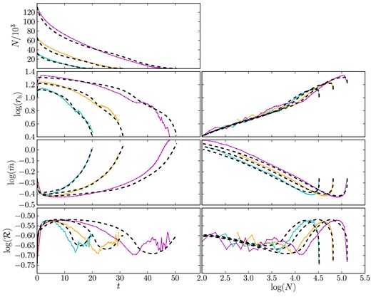
Comparison of the emacss model described in Sections 4–6 to N-body data for a series of RV filling N-body simulations of clusters in tidal fields. The clusters are located within an isothermal galaxy halo with VG = 220 km s−1, at RG = 15 kpc. The left column plots N, rh, |$\bar{m}$|, and |$\mathcal {R}_{\rm hJ}$| as a function of time, while the right column plots the same properties as a function of log (N). The initial conditions of the N-body simulations are described in Section 2, with N0 = 128 k (cyan track; longest surviving), N0 = 64 k (magenta), N0 = 32 k (orange) stars. The clusters are allowed to evolve until their eventual dissolution. For these SCs, |$\mathcal {R}_{1}\simeq 0.19$|. The observed discrepancies are most likely effects of the (simplified) definitions of find and γe, which follow from the fact that simulations show the highest RV filling and consequently the fastest induced escape.
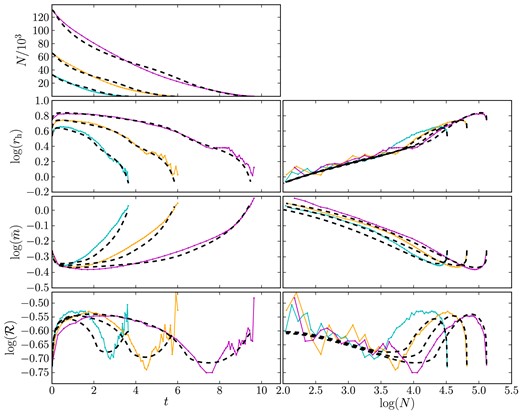
Same as Fig. A1 but for clusters located at RG = 2.8 kpc.
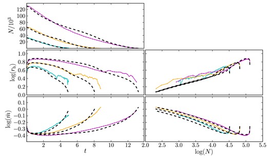
Same as Figs A1 and A2 but clusters on e = 0.5 eccentric orbits with apocentre RA = 8.5 kpc. The three clusters shown have initial rh chosen to be RV filling, such that |$\mathcal {R}_{1}\simeq 0.19$|. In these simulations, we have used the approximation of Baumgardt & Makino (2003), and have therefore approximated the eccentric orbit as a circular orbit at radius RG = RA(1 − e) (see Section 3.4). We find that emacss predicts mass loss and total lifetime extremely well, although during the balanced phase the half-mass radius is under-predicted by a factor of ≲2. While this factor is comparable with the case of a circular orbit, we find increasing discrepancies between N-body simulation of emacss prediction for higher eccentricities (e.g. ≳2 in rh, or ≃1000 in N for e = 0.8). However, such uncertainty is comparable with the assumptions made for statistical studies of observational SCs (e.g. see Alexander & Gieles 2013; Shin et al. 2013). We suggest that the under-prediction of radius occurs since the clusters spend a substantially greater fraction of their lifetime near apocentre, where the cluster can expand further than predicted by our circular orbit approximation. As the cluster passes through apocentre, stars are stripped away (hence leading to our correct mass-loss description), while the rapidly varying tidal field strength causes adiabatic shocking in the cluster (e.g. see Weinberg 1994a,b). The consequence of this injection of energy is expansion, according to equation (34), with comparatively few escapers due to the weaker tidal field.
