


Abstract
Microlensing observations indicate that quasar accretion discs have half-light radii larger than standard theories predict. The observations of Blackburne and colleagues suggest that these half-light radii may have a weak wavelength dependence. We consider disc temperature profiles that might match these observations. Nixon and colleagues have suggested that misaligned discs around spinning black holes can have annuli torn off them at radii where the Lense–Thirring torque overcomes the disc's viscosity. These annuli precess, spread radially, and intersect with the remaining disc, heating the disc at potentially large radii. However, unless the intersections occur at an angle of <1°, highly supersonic collisions will shock heat intersecting gas to T ∼ 107 K. Discs with such shock-heated regions have significantly larger half-light radii, but are overluminous in X-rays. If instead heating occurs through intermittent weak shocks, the X-ray luminosities are consistent with observations but the half-light radii are not significantly larger. We also study two phenomenological disc temperature profiles. Discs with a temperature spike at relatively large radii and lowered temperatures at radii inside the spike yield improved and acceptable fits to microlensing sizes in most cases. Such temperature profiles could in principle occur in sub-Keplerian discs partially supported by magnetic pressure. However, such discs overpredict the fluxes from quasars studied with microlensing except in the limit of negligible continuum emission from radii inside the temperature spike.
1 INTRODUCTION
Quasar accretion disc half-light radii can be inferred using observations of gravitationally lensed quasars (see e.g. Wambsganss 2006). Microlensing by stars in the lensing galaxy causes the flux ratios of the lensed images to deviate from the predictions of models with smooth mass distributions. The amplitude of these deviations depends on the size of the emission region at the wavelength being observed relative to the typical Einstein radius of the lensing stars.
Observationally, it has been found that quasar accretion discs have microlensing sizes (inferred from microlensing observations) which are larger than the thin disc theory sizes (Morgan et al. 2010) predicted using each quasar's estimated BH mass and assuming accretion at the Eddington rate, 10 per cent accretion efficiency and an average disc inclination to the line of sight of 60°. In the three studies to date with sample sizes of 10 or more objects, the microlensing sizes range from a factor of ∼1.8 ± 1.6 higher on average at mean rest-frame wavelength 2660 Å (Morgan et al. 2010, hereafter M10) to a factor of |${\sim } 5_{-4}^{+3}$| (Jiménez-Vicente et al. 2012) to |${\sim } 10^{+7}_{-5}$| (Blackburne et al. 2011, hereafter B11)1 higher on average at mean rest-frame wavelength 1736 Å.
The above results show that microlensing sizes are larger than theory sizes at only marginal significance (assuming accretion at the Eddington limit, which may be an overestimate; see Kollmeier et al. 2006). However, microlensing sizes are significantly larger than quasar flux sizes (M10). Flux sizes are found by determining how large a standard disc would need to be to generate the specific luminosity corresponding to the observed magnification-corrected flux of the quasar at a given wavelength. M10 find that microlensing sizes are ∼4 ± 2 times larger than flux sizes. Similar results have been obtained in studies of individual objects (e.g. Morgan et al. 2008, 2012; Dai et al. 2010; Poindexter & Kochanek 2010; Mediavilla et al. 2011).
As for the wavelength dependence of quasar half-light radii, the microlensing sizes in the study of B11 are very weakly dependent on wavelength in 10 of 11 cases studied, implying in the simplest case a temperature profile steeply decreasing with radius at temperatures that generate ultraviolet emission. On average, B11 find R1/2 ∝ λν with ν = 0.17 ± 0.15 ± 0.13 (quoting random and systematic errors), where ν = 4/3 is predicted by theory. The only published study besides that of B11 which includes size measurements of more than one quasar at more than one wavelength is that of Jiménez-Vicente et al. (2014), who study one image pair in each of eight lensed quasars (and three image pairs in another lensed quasar) and find ν = 0.8 ± 0.2. For the only quasar in both samples (HE0435−1223), they find |$\nu =0.75_{-0.4}^{+0.8}$| while B11 find ν = 0.67 ± 0.55.
The results of B11 that 10 of 11 objects considered have ν < 4/3 can also be contrasted with studies of six individual objects which have found values consistent with ν = 4/3 in at least five of six cases. Four studies have utilized multi-epoch photometry to study microlensing sizes as a function of wavelength in three quasars, finding for HE 1104−1805 |$\nu =1.64_{-0.42}^{+0.63}$| (Poindexter, Morgan & Kochanek 2008) and |$\nu =1.0_{-0.56}^{+0.30}$| (Blackburne et al. 2013), ν = 1.2 ± 0.3 for Q 2237+0305 (Eigenbrod et al. 2008), and ν = 1.3 ± 0.3 for HE 0435−1223 (Mosquera et al. 2011), as compared to ν = 0.67 ± 0.55 for that object in B11. Three single-object studies have utilized single-epoch photometry in a similar fashion to B11 to infer a quasar's microlensing size as a function of wavelength, finding |$\nu =1.48_{-0.43}^{+0.60}$| for MG 0414+0534 (Bate et al. 2008), as compared to ν = 1.50 ± 0.84 for that object in B11, ν = 1.0 ± 0.5 for SBS 0909+532 (Mediavilla et al. 2011), ν < 4/3 at 94 per cent confidence for SDSS J0924+0219 (Floyd, Bate & Webster 2009), as compared to ν = 0.17 ± 0.49 for that object in B11.
In this admittedly small number of studies, there is no statistically significant difference between the single-object ν values derived from single-epoch photometric studies and those derived from multiple-epoch studies.2 Nonetheless, the values of ν measured in the sample of B11 are on average lower than those measured in the studies quoted above. Further studies of microlensed quasars (e.g. Mosquera & Kochanek 2011) are clearly needed to determine whether the values of ν measured by B11 are correct by measuring ν for the same objects using different methods. Meanwhile, investigation of plausible explanations for unexpectedly large sizes and possible non-standard temperature profiles in quasar accretion discs is warranted, and we undertake such an investigation herein.
To summarize: there is marginal evidence that quasar accretion discs are larger than their theory sizes (though the evidence strengthens if quasars are not typically accreting at the Eddington limit), considerable evidence that they are larger than their flux sizes, and possible evidence that their half-light radii have a shallower wavelength dependence than is predicted by theory, implying a steeper temperature profile than predicted. As discussed in M10, a complication to the latter issue is that reconciling the three size measurements may require flatter temperature profiles (β < 3/4, which may help explain the ultraviolet spectral slope of quasars; see Gaskell 2008). The two constraints are not necessarily contradictory; a non-monotonic temperature profile can be locally steep yet effectively flat overall. If the correct temperature profile and physical parameters are used, theory sizes and flux sizes should agree with each other and with the microlensing sizes and the observed wavelength dependence of the sizes should match that predicted by the temperature profile.
Other options discussed in M10 to explain discrepant size measurements include low accretion efficiency for unobscured quasars or increasing the apparent disc size through contamination by line emission arising on larger physical scales or through scattering (see also Dai et al. 2010). For example, a large fraction of the disc continuum could be intercepted by a strongly warped disc (e.g. Nayakshin 2005; Tremaine & Davis 2013). In that case, the half-light radius will increase with a wavelength dependence related to the disc albedo, as radiation not scattered by the disc will be absorbed and reradiated at the local equilibrium temperature (which will be lower than the characteristic temperature of the continuum emission from smaller radii).
Disc sizes also increase with Eddington ratio, so super-Eddington accretion may also help explain discrepant size measurements. Furthermore, Abolmasov & Shakura (2012) have suggested that the steep temperature profile found by B11 arises from the formation of a scattering photosphere in gas outflowing from the inner regions of an accretion disc undergoing super-Eddington accretion (see also Bonning et al. 2013; Sutton, Roberts & Middleton 2013). The small size of the X-ray emitting regions in quasars (e.g. Morgan et al. 2012) could be explained in their model if the outflowing gas forms a Compton-thick funnel-shaped wind and photosphere, so that quasars are only visible within the cone of the funnel because the funnel obscures both the X-ray and UV continuum source regions when viewed from other angles.
Another possible explanation for the temperature profiles found by B11 may arise from changes to an accretion disc resulting from misalignment of its initial angular momentum vector and the angular momentum vector of a spinning BH. Any material in the vicinity of a massive spinning object experiences a precession induced by the frame dragging due to the object (Lense & Thirring 1918). The result of this precession, known as the Lense–Thirring effect, on a misaligned disc around the object is that each individual ring in the disc will precess at different rate, warping the disc.
Bardeen & Petterson (1975) showed that the discs around spinning BHs evolve in such a way that in the final configuration the disc is warped, with the orbital angular momentum of the inner region either aligned or anti-aligned with the spin axis of the BH while the disc's outer region remains unperturbed. Warped-disc dynamics has been the subject of extensive research (e.g. Papaloizou & Pringle 1983; Kumar & Pringle 1985; Pringle 1992; Papaloizou & Lin 1995; Ogilvie 1999; Lubow, Ogilvie & Pringle 2002).
In several recent papers (Nixon & King 2012; Nixon, King & Price 2012a; Nixon et al. 2012b, hereafter NKPF; Nixon & Salvesen 2014), it has been suggested that the inner regions of inclined discs could evolve by tearing apart instead of smoothly warping. NKPF showed that for realistic parameters, the inner region of randomly oriented accretion discs around a spinning BH will tear, due to the Lense–Thirring effect. If the angle between the outer disc and the BH spin is in the range ∼ 45°-135°, the misalignment between the inner edge of the outer disc and the annulus (of width ∼H) torn-off will be >90° after half a precession period. The rotational velocities of those gas parcels will then be partially opposed, leading to cancellation of angular momentum and rapid infall (see Nixon et al. 2012a). NKPF suggested that, given the smallness of the misalignment angle upper limit for avoiding disc tearing (of order a few degrees), the effect should be common in accretion around the supermassive BHs that power quasars.
When gas in a precessing annulus torn from a disc intersects with gas in an annulus still connected to the disc, the intersecting gas will be collisionally heated. High-temperature gas in intersection regions at relatively large distances from the central BH can in principle help explain the large, relatively wavelength-independent half-light radii inferred for quasar accretion discs. In addition, the wide range of behaviours possible in the torn disc model as a function of the initial disc–BH spin misalignment angle could in principle help explain the wide range of wavelength dependences in quasar accretion disc half-light radii (B11).
In this paper we examine whether the temperature profiles of torn and other non-standard discs can simultaneously reproduce the observed spectral energy distributions (SEDs) and inferred large half-light radii of quasar accretion discs. In Section 2 we outline the initial torn disc model used in our study. In Section 3 we discuss the temperature profiles and SEDs for selected torn discs. In Section 4 we explore a small set of additional temperature profiles. We discuss our results in Section 5. Where necessary, we assume a flat universe with ΩM = 0.3, |$\Omega _\Lambda =0.7$|, and H0 = 70 km s−1 Mpc−1.
2 TORN DISC TOY MODEL
Our initial model begins with accreting material forming a Keplerian disc at large radii from the BH. The disc's spin axis is oriented at a random angle 0° < θ < 180° relative to the BH spin axis.
The disc spreads inwards and different annuli in it precess at different rates due to the Lense–Thirring effect, so the disc warps as it spreads inwards. The disc eventually reaches a radius where viscous dissipation cannot overcome the shear between adjacent annuli imposed by the Lense–Thirring effect. The innermost annulus of the disc then tears away from the rest of the disc and precesses independently. This annulus has width ∼H, where H is the local disc height.
There will be two contact points between the precessing annulus and the next innermost annulus (which forms the inner edge of the outer disc). At these points gas from each annulus on intersecting orbits is likely to shock, converting some orbital motion to heat. The post-shock gas will be unable to remain in circular orbits at the intersection radius. The original NKPF picture consists of gas intersecting at angles up to 2θ.
2.1 Break radius and circularization radius
2.2 Shock heating
If gas is shock heated to a temperature higher than the Compton temperature of the ambient radiation field, the gas will cool by transferring its thermal energy to the radiation field through inverse Compton scattering. The Compton temperature of a quasar radiation field is ∼107 K (equations 25 and 26 of Sazonov, Ostriker & Sunyaev 2004). We therefore cap the value of Tsurf at 107 K.
3 TORN DISC TOY MODEL SEDs AND HALF-LIGHT RADII
The temperature profile and SED of a torn disc ultimately depend on the disc/BH spin misalignment angle θ, the dimensionless BH spin parameter a (0 ≤ a ≤ 1),3 the dimensionless viscosity parameter α, the disc height to radial distance ratio H/R, and the BH mass MBH and normalized mass accretion rate |$\dot{M}c^2/L_{\rm Edd} \propto \dot{M}/M_{\rm BH}$|. B11 write this latter quantity as fEdd/η, where the Eddington ratio is |$f_{\rm Edd}=L_{bol}/L_{\rm Edd} =\dot{M}/\dot{M}_{\rm Edd}$| and the accretion efficiency is |$\eta =L_{{\rm bol}}/\dot{M}c^2$|. B11 assumed η = 0.15 and fEdd = 0.25, whereas in all cases we assume a Schwarzschild BH (η = 0.057). To match the value of fEdd/η used by B11, we assume fEdd = 0.1. We also assume H/R = 1.7 × 10⁻³ (so that the disc height at any radius is H = 1.7 × 10⁻³R), α = 0.1, and MBH = 109M⊙. In our illustrative calculations below, we adopt a SS73 temperature profile (valid only for a = 0) even for the case of a ≠ 0, as our arguments are insensitive to the differences between SS73 and NT73 SEDs.
3.1 Single-Rb case
Equations (4), (5) and (7) generate a family of temperature profiles as a function of θ which consist of:
a normal SS73 disc (Tsurf = TSS73) at R < Rcirc(θ),
a gap at Rcirc < R < Rb(θ) − H(Rb),
a shock-heated region (Tsurf = TSS73 + ΔT) at radii Rb − H(Rb) < R < Rb + H(Rb),
and a normal SS73 disc again at R > Rb + H(Rb).
To find the temperature profile for the scenario put forth by NKPF, in which the precessing disc intersects with its neighbouring annulus over half to one precession periods, for a given θ we use equation (7) to calculate Tsurf(Rb) = TSS73(Rb) + ΔT(Rb) for η = θ (θ ≤ 90°) or η = 180° − θ (θ ≥ 90°), as the average of η over one precession period is about half the maximum η.
We then calculate SEDs and half-light radii using the Lλ values from the regions R < Rcirc, Rb − H < R < Rb + H and R > Rb + H, assuming thermal emission from optically thick gas in all regions.
Fig. 1 shows an SS73 disc SED and the SEDs resulting from these shock-heated disc temperature profiles. The SEDs are much bluer and more X-ray luminous than observed quasar SEDs. (Note that the SS73 disc model is known to be a poor fit to observations at λ ≲ 1000 Å, and that at X-ray wavelengths an additional power-law component is needed in addition to thermal disc emission. Those wavelengths are plotted here to examine if an SED overpredicts the short-wavelength emission, not in expectation of a good fit at short wavelengths from any SED, even a baseline SS73 one.)
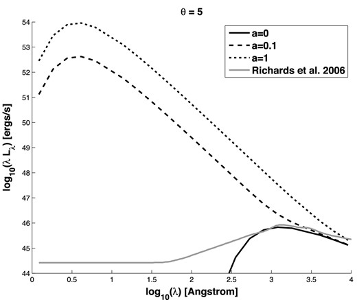
SEDs of accretion discs with MBH = 109 M⊙ and fEdd = 0.1. The solid black line is the SED of an accretion disc with a = 0. The dashed and dotted lines show the SEDs of discs tilted by θ = 5° from the spin axis of BHs with a = 0.1 and 1, respectively, that tear and shock heat to T = 107 K at Rb over an annulus of width 2H(Rb). The grey line is the mean quasar SED from Richards et al. (2006).
We have assumed that an entire annulus at Rb is at the post-shock temperature, but it may be more accurate to assume that only the two intersection regions of surface area (2H)2 on each face of the disc are at that temperature. Fig. 2 shows the SEDs in that case; they are still much bluer and more X-ray luminous than observed quasar SEDs. However, we note that if the local cooling time is short enough, the effective post-shock temperature may be lower than the peak shock-heated value we assume. This complication is beyond our toy model and so we do not consider it here.
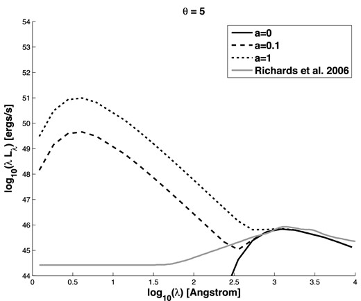
Same as Fig. 1, except that shock heating occurs only in the intersecting regions of the torn annulus and the adjacent annulus that forms the inner region of the outer disc.
We do not model the thermal and radiation pressure associated with such strong, high-temperature shocks, which would likely prove disruptive to the disc farther out. It is sufficient for our purposes to note that if the disc is disrupted then this toy model cannot explain the sizes of steady-state discs, while if the disc is somehow not disrupted then its SED in this toy model will not match observations.
We discuss the half-light radii results for this and the next model in Section 3.3.
3.2 Small-η case
Large intersection angles between the precessing annulus and the outer disc lead to high-temperature shock-heated regions and SEDs which in this toy model is inconsistent with a standard quasar SED. A more plausible alternative picture is one in which the intersection angle never becomes large.
As the annulus at Rb starts precessing, the intersection angle between it and the next annulus out will grow with time. The relative velocity between those annuli will also grow with time. Shock heating between the two annuli will happen once the magnitude of their relative velocity is sufficiently large, rather than at the maximum relative velocity possible for that value of θ. Therefore, the relative velocity at the time of intersection may not depend on θ, and the shock-heated temperature may be considerably lower than 107 K.
We now imagine a different scenario for a disc oriented at θ. An annulus breaks off at Rb(θ), precesses by η = 0| $_{.}^{\circ}$|1, shocks, and reorients itself and its adjacent annulus to θ − 0| $_{.}^{\circ}$|05. Part of this reoriented annulus will be subject to breaking at Rb(θ − 0| $_{.}^{\circ}$|05), as the separation between the two break radii will be less than H for most θ.
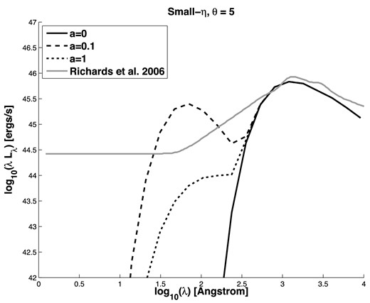
The solid black line is the SED of an accretion disc with a = 0. The dashed and dotted lines show the SEDs of discs tilted by θ = 5° from the spin axis of BHs with a = 0.1 and 1, respectively, that tear and shock heat in multiple, short-lived shocks, each with intersection angle η = 0| $_{.}^{\circ}$|1. See Section 3.2 for a discussion of why the a = 1 curve and not the a = 0.1 curve is most similar to the a = 0 curve. The grey line is the mean quasar SED from Richards et al. (2006).
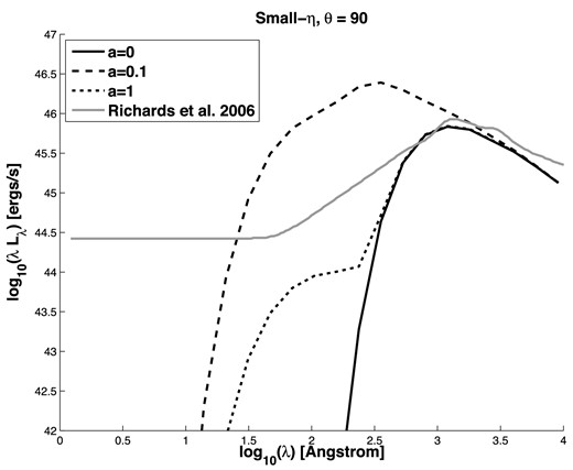
Same as Fig. 3, except for θ = 90°.
Note that the SEDs in the small-η scenario could in principle be consistent with the range of observed quasar SEDs if most BHs are rapidly spinning, so that cases with a ≫ 0.1 in Figs 3 and 4 were much more common than cases with a ≲ 0.1. (The first test of that possibility would be to see if the SEDs are relatively unchanged when calculated assuming an NT73 disc with the appropriate value of a instead of an SS73 disc.) However, the SEDs predicted for low spins (a ≈ 0.1; consistent with the accretion picture of King & Pringle 2006, 2007) do show a soft X-ray component which has recently been shown to be ubiquitous in type 1 AGN (Scott, Stewart & Mateos 2012).
3.3 Torn disc toy model results
Table 1 gives the half-light radii at λ = 1736 Å inferred by B11 (microlensing sizes) and calculated for the scenarios considered in this section (theory sizes), all for quasars of mass MBH ≃ 109 M⊙.
Model accretion disc half-light radii at λ = 1736 Å.
| Model | Shocked region | a | θ(°) | log (r1/2in cm) |
|---|---|---|---|---|
| Inferred (B11) | – | – | – | 15.97−16.61 |
| SS73 | None | 0 | – | 15.55 |
| Single-Rb torn disc | Full annulus | 0.1 | 5 | 15.19 |
| Single-Rb torn disc | Full annulus | 0.1 | 90 | 15.90 |
| Single-Rb torn disc | Full annulus | 1 | 5 | 15.86 |
| Single-Rb torn disc | Full annulus | 1 | 90 | 16.56 |
| Single-Rb torn disc | Intersections only | 0.1 | 5 | 15.55 |
| Single-Rb torn disc | Intersections only | 0.1 | 90 | 15.98 |
| Single-Rb torn disc | Intersections only | 1 | 5 | 15.56 |
| Single-Rb torn disc | Intersections only | 1 | 90 | 16.56 |
| Small-η torn disc | Intersections only | 0.1 | 90 | 15.64 |
| Small-η torn disc | Intersections only | 0.3 | 90 | 15.59 |
| Small-η torn disc | Intersections only | 1 | 90 | 15.56 |
Most torn disc cases have larger half-light radii than the SS73 case. However, only the single-Rb, a = 1, θ = 90° torn disc cases (with a shocked region over the full annulus or at the intersections only) have half-light radii large enough to match the observationally inferred results of B11.4 Within the uncertainties, single-Rb torn discs with full-annulus shocked regions around BHs with a = 1 might match the observed range of r1/2 for a reasonable distribution of angles θ. However, those scenarios do not produce SEDs consistent with observations. And while the small-η scenarios are consistent with observed SEDs for certain parameter choices, none of those scenarios result in half-light radii large enough to match the observations when averaged over a reasonable range of θ values.
These conclusions hold if fEdd is increased from 0.1 to 1.0. In that scenario the temperature of the disc will be higher at all radii (equation 1), increasing log (r1/2) by 0.33 in the SS73 case (equation 2), which reduces but does not eliminate the size discrepancy. However, because H/R increases with fEdd (SS73 equation 2.8), the values of Rb for torn discs will shrink as fEdd increases (equation 4). That will lead to smaller values of log (r1/2) for torn discs in cases where the shocked region dominates the emitted flux and values of log (r1/2) only 0.33 higher in most other cases.
Lastly, we note that this toy model is a simple description of torn discs and that further work is needed to realize the full dynamics and observational properties of this mode of accretion.
4 PHENOMENOLOGICAL MODEL TESTS
In this section we consider whether better matches to observations can be obtained with two phenomenological models for disc temperature profiles that do not involve torn discs. These models are energetically plausible but are not rigorously derived; our intention is simply to explore how well simple combinations of an underlying disc and a temperature spike can match observations.
We consider the constraints placed on these two phenomenological models by the quasar accretion disc half-light radii inferred by B11 (microlensing sizes; see Section 1). B11 characterize the half-light radius’ dependence on wavelength in their sample as r1/2 = λν, with ν = 0.17 ± 0.15. The quantity ν is related to the slope β of a disc temperature profile T(R) ∝ R−β as β = ν−1; thus, B11 constrain |$\beta \simeq 6_{-3}^{+\infty }$|.
The weak dependence of the half-light radii on wavelength seen by B11 extends over the wavelength range 0.1-1 μm, corresponding to wavelengths of light emitted by blackbodies at temperatures of approximately 3000 < T < 30 000 K.
Therefore, one simple explanation for the results of B11 is that quasar accretion discs contain a region where the temperature drops from T ≳ 30 000 K to T ≲ 3, 000 K following a power law of the approximate form T(R) ∝ R−β with |$\beta \simeq (6_{-3}^{+\infty })$|.5
We parametrize our models in terms of MBH (fixed for each quasar), the Eddington ratio fEdd (for which we test a wide range of values), and other parameters appropriate to each of the two models we now present.
4.1 Forming disc model
Tabulated and derived parameters for quasars from B11.
| Lbol,opt | σ(log | Measured | SS73 | log (rI), | log (rI), | ||||
|---|---|---|---|---|---|---|---|---|---|
| MBH | (1046 | Lbol, opt) | log 〈r1/2〉 | log (rQ) | log 〈r1/2〉 | β = 3/4 | MR best fit | σr/σ | |
| Quasar | (109 M⊙) | erg s−1) | (log erg s−1) | (cm) | (cm) | (cm) | (cm) | (cm) | |
| HE 0230−2130 | 0.092 | 0.29 | 0.29 | 16.57 | 16.76 | 15.13 | 14.73 | 16.73 | 0.148 |
| MG J0414+0534 | 1.82 | 3.6 | 0.22 | 15.94 | 16.81 | 16.05 | 14.28 | 14.38 | 0.278 |
| HE 0435−1223 | 0.50 | 0.38 | 0.31 | 16.07 | 16.79 | 15.72 | 14.95 | 15.11 | 0.390 |
| RX J0911+0551 | 0.80 | 1.3 | 0.23 | 16.19 | 16.80 | 15.69 | 14.86 | 15.12 | 0.324 |
| SDSS J0924+0219 | 0.11 | 0.06 | 0.60 | 15.73 | 16.77 | 15.30 | 14.64 | 14.88 | 0.530 |
| HE 1113−0641 | 0.087 | 0.27 | 0.31 | 15.82 | 16.76 | 15.34 | 14.76 | 14.86 | 0.997 |
| PG 1115+080 | 1.23 | 1.1 | 0.41 | 16.69 | 16.81 | 15.99 | 15.21 | 15.59 | 0.626 |
| RX J1131−1231 | 0.06 | 0.08 | 0.24 | 15.51 | 16.76 | 15.36 | 14.88 | 14.94 | 0.342 |
| SDSS J1138+0314 | 0.04 | 0.38 | 0.31 | 15.98 | 16.75 | 14.83 | 14.64 | 15.05 | 0.944 |
| SDSS J1330+1810 | 1.5 | 4.7 | ... | 16.13 | 16.81 | 16.12 | 14.24 | ... | ... |
| WFI J2026−4536 | 0.79 | 2.5 | 0.31 | 16.42 | 16.80 | 15.77 | 15.03 | 15.41 | 0.474 |
| WFI J2033−4723 | 0.18 | 0.57 | 0.17 | 16.69 | 16.77 | 15.42 | 14.90 | 15.16 | 0.508 |
Values of MBH and Lbol,opt are taken from table 8 of B11. Uncertainties on Lbol,opt are discussed in Section 4.3. The measured log 〈r1/2〉 column gives the average of each object's log-prior, median r1/2 values from B11. The rQ values are discussed in Section 4.1. The SS73 〈r1/2〉 calculations used fEdd = 0.1 to match B11 given our assumed value of η (see Section 3). The rI flux sizes are discussed in Section 4.4, for both the β = 3/4 case and the best-fitting MR model. The σr/σ values are discussed in Section 4.3.
The values these parameters can take are constrained by energy conservation. The energy per second emitted from the disc in its forming region (R > Rb) must be no more than the energy available to the mass per second which has reached that radius from infinity. Consider the limiting case of the forming disc model, which consists of gas falling radially inward in the disc plane until it reaches Rb, at which point it circularizes on to the inner disc with kinetic energy per unit mass |$\frac{1}{2}v^2 = \frac{1}{2}GM_{\rm BH}/{R_{\rm b}}$|. The potential energy per unit mass gained by reaching Rb is GMBH/Rb. Thus, the forming region of the disc (R > Rb) can emit energy at a rate |$L\le \frac{1}{2}G\dot{M}M_{\rm BH}/{R_{\rm b}}$|, with the characteristic width and peak temperature of the extraction region dependent on β.
For this model we test values of β from 1 to 18, fEdd from 0.01 to 1, Thi from 10 000 to 70 000 K, and Rb = R(Tlo) with Tlo from 4000 K < Tlo < 28 000 K. We detail our results on this model and the next in Section 4.4.
4.2 Magnetically restrained disc models
A disc will have greater viscous dissipation (and thus higher temperatures) than a Keplerian disc if gas flowing inward through a disc has a rate of change of azimuthal speed with radius whose absolute magnitude is greater than that experienced in a Keplerian disc. If the magnitude of the rate of change in azimuthal speed is less than in the Keplerian case, the annulus will have a lower temperature than in the Keplerian case.
Both situations can occur (at different radii) in discs where magnetic pressure is important. Ogilvie (1997) has shown that a disc threaded by a strong poloidal magnetic field can have an angular velocity with order unity deviations from the Keplerian value. In the magnetically arrested disc model of Narayan, Igumenshchev & Abramowicz (2003), a strong poloidal magnetic field disrupts disc accretion at some radius, inside of which gas accretes at much less than the free-fall velocity (see also McKinney, Tchekhovskoy & Blandford 2012). We consider a range of ‘magnetically restrained’ (MR) models where gas accreting through a Keplerian disc at large radii reduces its orbital velocity to a fraction f < 1 of the circular velocity at Rb by the time it reaches radius Rb (increasing the local disc temperature in the process) and continues to orbit at a fixed fraction f of the Keplerian circular velocity vK at R < Rb; that is, f = constant = vorb(R)/vK(R) for all R < Rb. (Sub-Keplerian rotation is required in the inner region to ensure that gas moves inward at Rb instead of being flung outward.) Assuming that the radial velocities in the disc at R < Rb are still much less than the rotational velocities, the sub-Keplerian rotation reduces the dissipational heating at R < Rb, leading to temperatures at R < Rb which are |$\sqrt{f}$| times the temperatures in an SS73 disc with the same parameters. The combined profile has a cooler inner disc and warmer outer disc than in the forming disc model.
The values of these parameters are constrained by the fact that the disc has a fraction (1 − f 2) of the kinetic energy of the accreting gas at Rb available to emit as heat at R > Rb, in addition to the normal disc emission (|$\propto T_{\rm SS73}^4$|) at R > Rb. We derive the relationship between the parameters of this model in Appendix B (equation B5), and require all combinations of parameters we test to satisfy that relationship.
For these MR models we test the same parameter space of fEdd, Thi, Rb and β used for the forming disc model, plus values of f given by f = 0 and f = 0.01n2 for n = 2 to 9. We detail our results on this and the previous model in Section 4.4.
4.3 Random and systematic errors
For each quasar in B11, for a specific model and set of model parameters including that quasar's MBH we calculate half-light radii at the observed wavelengths and a bolometric luminosity at λ < 1μm. We then calculate the χ2 value of the model using the model and observed log Lbol, opt values from Pooley et al. (2007) and B11 and the model and inferred half-light radii. Most quasars have their half-light radius measured at eight wavelengths; thus, the half-light radius has eight times greater weight in the χ2 calculation than Lbol,opt does.
Inspection of fig. 6 of B11 shows that the error bars for a given object are generally larger than the scatter between points. Using those error bars would lead to misleadingly small χ2 and |$\chi ^2_\nu$| values. The σ values used in fig. 6 of B11 incorporate both random and systematic error, added together in quadrature as |$\sigma = \sqrt{\sigma _r^2+\sigma _s^2}$|. Adding random and systematic errors together can lead to erroneous results, but is likely an adequate approximation in in this case. The systematic errors considered by B11 were apparent flux ratio deviations arising from emission-line contamination of the observed magnitudes, confusion with adjacent objects on the images, and variability from time delays. Only the latter source of uncertainty is likely to systematically bias the half-light radii at all wavelengths in the same direction; emission-line contamination will vary between filters, and confusion with adjacent objects will vary with the colour of the objects. While we first consider only σr in our χ2 calculations, we also show the results of a conservative approach in which we consider the full σ.
To calculate the σr values, we assume that each quasar's total error in r1/2 in each filter (table 7 of B11) can be broken down into random and systematic errors, in proportion to the contribution of random and systematic errors to the uncertainties for all data points for that quasar (table 5 of B11). From the ratio σr/σs we determine the ratio σr/σ for each quasar (Table 2). The r1/2 error values used in our χ2 calculations are the quasar's uncertainties σ from table 7 of B11 multiplied by the quasar's ratio σr/σ from Table 2.
The uncertainty on Lbol,opt stems from both the uncertainty in estimating Lbol,opt and the uncertainty in the total magnification of the lensed quasar. Pooley et al. (2007) considered the former source of error, and that source's contribution to σ(log Lbol,opt) here equals the σ(log MBH) quoted there (for quasars not in their sample, we adopt their average value of σ(log MBH) = 0.26 as a representative error on log Lbol,opt). For the latter source of error, we find five lenses for which the modelled image magnifications in table 6 of B11 can be compared with magnifications given in the discovery paper of each lens. We find that the total magnifications in B11 are 9 ± 15 per cent higher than those in the literature. To be conservative, we add an additional ±9 per cent linearly and an additional ±15 per cent in quadrature to the uncertainties on Lbol, equivalent to adding ±0.04 linearly and ±0.06 in quadrature to the uncertainty on log Lbol. The final uncertainties used in our χ2 calculations are tabulated for each quasar in Table 2.
4.4 Phenomenological model results
For each quasar we calculate a temperature profile for all allowable combinations of the specified parameter values given for each model above. For each model – SS73, forming disc, and MR for values of f from 0 to 0.81 – we find the minimum χ2 value over all tested values of fEdd, Thi, Tlo and β. We plot the resulting half-light radii versus wavelength, temperature profiles, SEDs, and |$\chi ^2_{\rm min}$| values for each quasar individually in Figs 5–15 ; see the caption to Fig. 5 for details. We present the |$\chi ^2_{\rm min}$| values and best-fitting parameter values for the SS73, forming disc, and best-fitting MR models in Table 3. For ease of comparison with other size values, Table 2 presents I-band flux sizes rI for both the β = 3/4 case and the best-fitting MR models, calculated following Appendix C.
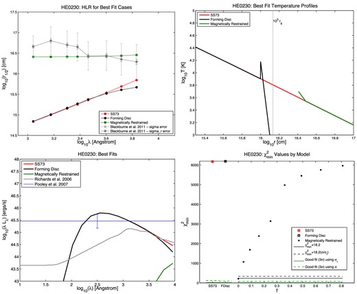
Half-light radius r1/2 versus wavelength (top left), temperature profile (top right), SED (bottom left), and |$\chi ^2_{\rm min}$| results (bottom right) for the quasar HE 0230. In the r1/2 plots, the measured points from B11 are shown in grey, with the random and full errors on each r1/2 value shown as the shorter and longer error bars, respectively. The best-fitting SS73 model is shown in red, the best-fitting forming disc model in black, and the best-fitting MR model in green. The same colours are used in the temperature profile plots. In the SED plots, the quasar's Lbol,opt value from Pooley et al. (2007) is shown as the horizontal blue line. The mean SED from Richards et al. (2006), summed from 102 to 104 Å, is normalized to that value as a reference for the typical shape of a quasar's ultraviolet/optical SED. In the |$\chi ^2_{\rm min}$| plots, the red open square on the left shows the SS73 disc |$\chi ^2_{\rm min}$|, the black open square next to it shows the forming disc |$\chi ^2_{\rm min}$|, and the circles show the |$\chi ^2_{\rm min}$| for the MR disc model at each value of f tested, where f = vorb/vK. The solid green line segments show, for each model, the upper limit for a statistically acceptable fit at the 99.73 per cent (3σ) confidence level, using the random errors only. The dashed green line segments show the same upper limit using the full errors quoted in B11. For the MR models, we use black lines to show the 3σ confidence limits for the five free parameters of the model (Δχ2 ≤ 18.2): at 99.73 per cent confidence, MR models underneath the black lines provide fits as statistically acceptable as the best fit found, using random errors only (solid black line) or the full errors from B11 (dashed black line). Note that we plot confidence limits for all five free parameters, not just one free parameter, because the best-fitting MR models as a function of f typically have differing values of the other parameters.
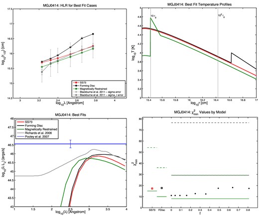
Same as Fig. 5, for quasar MG J0414.
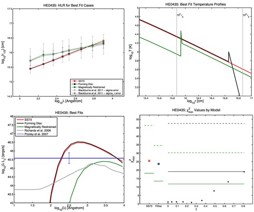
Same as Fig. 5, for quasar HE 0435.
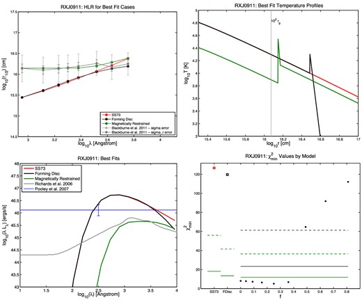
Same as Fig. 5, for quasar RX J0911.
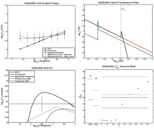
Same as Fig. 5, for quasar SDSS J0924.
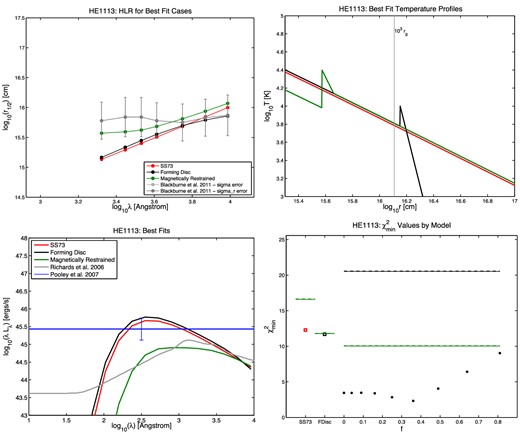
Same as Fig. 5, for quasar HE 1113.
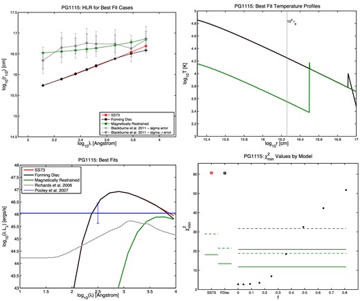
Same as Fig. 5, for quasar PG 1115.
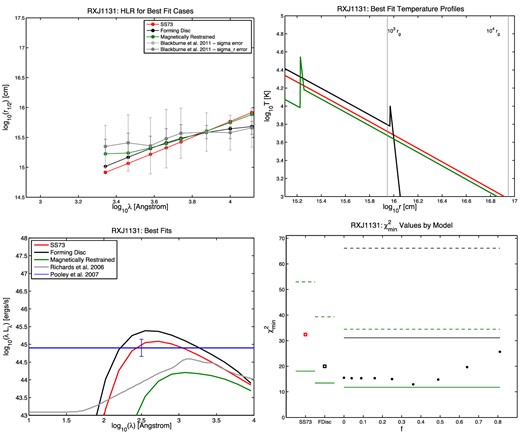
Same as Fig. 5, for quasar RX J1131.
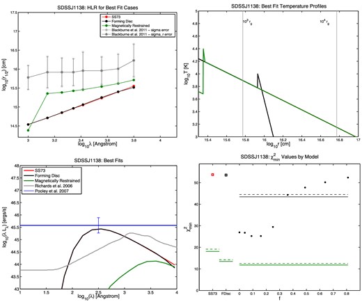
Same as Fig. 5, for quasar SDSS J1138.
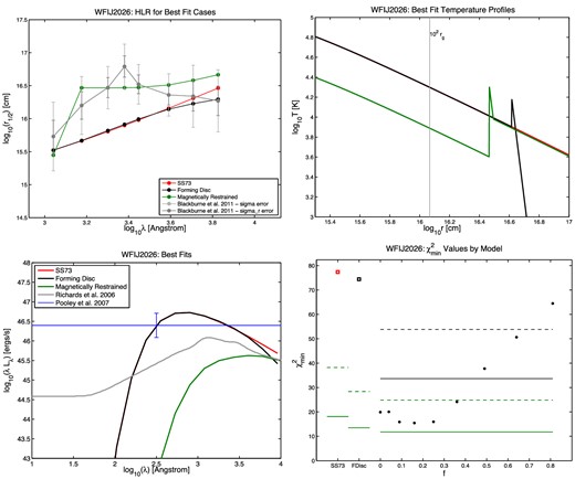
Same as Fig. 5, for quasar WFI J2026.
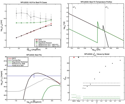
Same as Fig. 5, for quasar WFI J2033.
|$\chi ^2_{{\rm min}}$| results.
| Quasar | Parameter | SS73 | Forming disc | Magnetically restrained (f value, κλ value) |
|---|---|---|---|---|
| HE 0230−2130 | |$\chi ^2_{\rm min}$| | 6172.9 | 6193.8 | 213.6 (f = 0, κλ = 0.0001) |
| fEdd | 1 | 1 | 1 | |
| Lbol,opt (1046 erg s−1) | 1.051 | 1.057 | 0.003 | |
| β | 12 | 2 | ||
| Thi (K) | 15 000 | 5000 | ||
| Tlo (K) | 8000 | 4000 | ||
| MG J0414+0534 | |$\chi ^2_{\rm min}$| | 17.3 | 17.8 | 11.0 (f = 0.09, κλ = 0.6299) |
| fEdd | 0.06 | 0.07 | 0.03 | |
| Lbol,opt | 1.368 | 1.484 | 1.036 | |
| β | 12 | 3 | ||
| Thi | 10 000 | 60 000 | ||
| Tlo | 6000 | 28 000 | ||
| HE 0435−1223 | |$\chi ^2_{\rm min}$| | 25.5 | 23.6 | 0.9 (f = 0.25, κλ = 0.4841) |
| fEdd | 0.9 | 1 | 0.4 | |
| Lbol,opt | 3.972 | 4.532 | 0.423 | |
| β | 6 | 18 | ||
| Thi | 10 000 | 30 000 | ||
| Tlo | 6000 | 16 000 | ||
| RX J0911+0551 | |$\chi ^2_{\rm min}$| | 126.7 | 119.7 | 5.1 (f = 0.25, κλ = 0.3034) |
| fEdd | 1 | 1 | 0.4 | |
| Lbol,opt | 9.069 | 8.936 | 0.883 | |
| β | 12 | 18 | ||
| Thi | 20 000 | 35 000 | ||
| Tlo | 10 000 | 14 000 | ||
| SDSS J0924+0219 | |$\chi ^2_{\rm min}$| | 36.7 | 34.8 | 1.7 (f = 0.16, κλ = 0.3233) |
| fEdd | 1 | 1 | 0.3 | |
| Lbol,opt | 1.263 | 1.261 | 0.035 | |
| β | 6 | 12 | ||
| Thi | 10 000 | 25 000 | ||
| Tlo | 6000 | 12 000 | ||
| HE 1113−0641 | |$\chi ^2_{\rm min}$| | 12.3 | 11.7 | 2.3 (f = 0.36, κλ = 0.6451) |
| fEdd | 0.8 | 1 | 1 | |
| Lbol,opt | 0.699 | 0.798 | 0.197 | |
| β | 6 | 3 | ||
| Thi | 10 000 | 25 000 | ||
| Tlo | 6000 | 16 000 | ||
| PG 1115+080 | |$\chi ^2_{\rm min}$| | 60.7 | 60.6 | 2.7 (f = 0.04, κλ = 0.1753) |
| fEdd | 1 | 1 | 1 | |
| Lbol,opt | 13.892 | 13.718 | 0.956 | |
| β | 6 | 18 | ||
| Thi | 10 000 | 15 000 | ||
| Tlo | 6000 | 12000 | ||
| RX J1131−1231 | |$\chi ^2_{\rm min}$| | 32.4 | 20.0 | 12.9 (f = 0.36, κλ = 0.7578) |
| fEdd | 0.3 | 0.6 | 0.2 | |
| Lbol,opt | 0.206 | 0.275 | 0.032 | |
| β | 12 | 12 | ||
| Thi | 10 000 | 35 000 | ||
| Tlo | 6000 | 16 000 | ||
| SDSS J1138+0314 | |$\chi ^2_{\rm min}$| | 53.7 | 53.5 | 25.2 (f = 0.09, κλ = 0.1525) |
| fEdd | 1 | 1 | 1 | |
| Lbol,opt | 0.461 | 0.460 | 0.038 | |
| β | 6 | 12 | ||
| Thi | 10 000 | 25 000 | ||
| Tlo | 6000 | 12 000 | ||
| WFI J2026−4536 | |$\chi ^2_{\rm min}$| | 77.4 | 74.4 | 15.5 (f = 0.16, κλ = 0.1695) |
| fEdd | 1 | 1 | 0.9 | |
| Lbol,opt | 8.956 | 8.851 | 1.327 | |
| β | 12 | 12 | ||
| Thi | 15 000 | 20 000 | ||
| Tlo | 8000 | 10 000 | ||
| WFI J2033−4723 | |$\chi ^2_{\rm min}$| | 288.5 | 289.3 | 79.3 (f = 0.04, κλ = 0.1047) |
| fEdd | 1 | 1 | 1 | |
| Lbol,opt | 2.062 | 2.058 | 0.063 | |
| β | 6 | 6 | ||
| Thi | 10 000 | 15 000 | ||
| Tlo | 6000 | 8000 |
The first point to notice about the best fits is that the best-fitting SS73 and forming disc models usually have large fEdd (0.7 ≤ fEdd ≤ 1 in 9 out of 11 cases). Larger fEdd results in a larger accretion disc, making it easier to match the large inferred half-light radii. This effect is less pronounced in the best-fitting MR models; they have fEdd = 1 in 6 of 11 cases, but three of those are poor fits. (However, we have only considered face-on discs in our modelling. An inclined disc will have half-light radii smaller than it does when face-on, and given that quasar discs will have a non-zero average inclination angle, the true best-fitting fEdd of our objects in all models will, statistically, be somewhat larger than the values quoted.)
The second point to notice is that the forming disc model is never a significantly better fit than the SS73 model.
The third point to notice is that in 8 of 11 cases, the MR models can provide a fit which is better than the SS73 or forming disc fit and is also a statistically acceptable fit at the 99.73 per cent confidence level if the full errors σ from B11 are used in the χ2 calculations. (If the σr values are used instead, only in 5 of 11 cases are statistically acceptable fits found.)
Two of the cases without acceptable fits using σ, HE 0230 and WFI J2033, have unusual wavelength dependences of their half-light radii and are discussed below. The third case, SDSS J1138, has the lowest MBH and the largest ratio of Lbol,opt to MBH in our sample. The SS73 and forming disc models can match the luminosity of SDSS J1138, but not its large half-light radii, even with fEdd = 1. The MR models with fEdd = 1 can better match the shape of its half-light radius versus wavelength curve, but still cannot match their large values, and is a worse fit to the observed luminosity. The large |$\chi ^2_{\rm min}$| in this object could be reduced if future observations reveal that its MBH is larger than the value we adopt, which is quite plausible given the considerable uncertainties on MBH estimates (see e.g. the comprehensive review of Shen 2013). The same might be true of HE 0230 and WFI J2033, which in addition to the unusual wavelength dependences of their half-light radii have the next largest ratios of Lbol,opt to MBH in our sample.
However, Table 2 shows that the flux sizes of the best-fitting MR models are still about an order of magnitude smaller, on average, than the measured microlensing sizes. (They are larger than the flux sizes of a β = 3/4 disc by Δlog r1/2 = +0.37 on average.) The one exception is HE 0230−2130, which has a best-fitting MR model with f = 0, corresponding to negligible thermal emission within the radius of the temperature spike. Except in that case, our best-fitting MR models produce more flux than observed in these objects. Incorporating flux sizes as a constraint in the fitting might shift the best-fitting f values to f = 0 in many cases, as the χ2 minimum as a function of f is quite broad.
The best-fitting SS73 and forming disc models tend to overestimate Lbol,opt, while the best-fitting MR model tends to slightly underestimate it. Better constraints on the models might be obtainable by including multiwavelength SEDs for these quasars in the χ2 fits, rather than just the total Lbol,opt. In the cases of HE 0230, PG 1115 and WFI J2033, such constraints would considerably increase the χ2 of the best-fitting MR models; those best-fitting models have SEDs that peak closer to 104 than 103 Å. It is not clear if a MR model would still yield a low |$\chi ^2_{\rm min}$| for PG 1115 if measurements of its multiwavelength SEDs were available for consideration in the fitting.
There are some similarities among the eight acceptable MR model fits. Those best fits have 0.04 ≤ f ≤ 0.36, corresponding to temperatures between 20 and 60 per cent of the SS73 value. The best fitting β is 12 or 18, except for MG J0414 (β = 3). (Note that MG J0414 is also consistent with an SS73 or forming disc.) The best-fitting Tlo is between 12 000 and 16 000 K, again except for MG J0414 (Tlo = 28 000 K). The best-fitting Thi is between 25 000 and 35 000 K, except for MG J0414 (Thi = 60 000 K) and PG 1115 (Thi = 15 000 K). The best-fitting values of fEdd, however, range from 0.03 to 1.
The eight acceptable best-fitting temperature profiles are all MR models. Of those eight profiles, we can characterize six of them as having a temperature (40 ± 20) per cent of the SS73 value within the radius where the SS73 disc reaches (13 000 ± 3000) K, at which radius there is a temperature spike reaching (25 000 ± 10 000) K, which falls off as a power law ∝ R−(15 ± 3). (The plus-or-minus values quoted above span the range of values seen around the quoted central value in each quantity in the six profiles.)
Our results are not in contradiction with those of M10, who explored what range of β and inner disc radii could explain microlensing size estimates in their fig. 4 and equation 6 and concluded that β < 3/4 for small values of Rin. M10 did not explore values as extreme as the β = 6 found by B11, but as suggested by their fig. 4, to reconcile β ≫ 1 with microlensing size estimates would require a large increase in the radius Rin within which disc emission is suppressed. A large Rin is just what our results suggest.
4.4.1 Quasars with half-light radii which decrease with increasing wavelength
Two quasars in B11 (HE 0230 and WFI J2033) appear to have half-light radii that decrease with increasing wavelength, albeit with large uncertainties. A temperature profile which increases with radius and then abruptly decreases can in principle reproduce the sign of this trend. (Conceptually, such a temperature profile might arise if the accretion luminosity is dominated by a shock at some radius Rb, with cooling gas undergoing radial infall within Rb.)
The two quasars above have maximum Δlog r1/2 = −0.61 ± 0.54 and Δlog r1/2 = −0.45 ± 0.54, respectively, from λmin to λmax. However, a radially inverted temperature profile like that described above cannot explain changes in r1/2 greater than about Δlog r1/2 ≃ −0.15. That Δlog r1/2 corresponds to the case of a narrow temperature spike at r1/2(λmin) which generates all the luminosity at λmin, and a flat temperature profile within that radius which dominates the luminosity observed at λmax, yielding |$r_{1/2}(\lambda _{{\rm max}}) = \frac{1}{\sqrt{2}}r_{1/2}(\lambda _{\rm min})$|, so that |$\Delta \log r_{1/2} = -\log \sqrt{2} \simeq -0.15$|. A temperature profile increasing with radius within r1/2(λmin) will produce an even smaller Δlog r1/2 value. A temperature profile decreasing with radius within r1/2(λmin) before spiking to a high temperature at that radius will not match the observed smooth change in r1/2 with wavelength; such a temperature profile would yield r1/2 values decreasing and then increasing with wavelength.
B11 note that the anomalous wavelength dependence of these two objects’ size estimates might also be produced by unusual microlensing caustic patterns such as those found at the centre of an astroid caustic. (The magnification increases away from the centre of an astroid caustic, leading to larger flux anomalies for larger sources.) That explanation for these objects’ half-light radii seems more likely after consideration of the difficulty in reproducing the results with actual disc temperature profiles. We predict that further observations of these two objects will not show the anomalous size estimates, as long as the time baseline between old and new observations is sufficient for the unusual microlensing caustic pattern to have moved out of our line of sight to the continuum source.
5 DISCUSSION AND CONCLUSIONS
We have tested several energetically plausible quasar accretion disc temperature profile models against the large quasar accretion disc half-light radii inferred by B11 from microlensing observations.
We have shown that the temperature profiles from our toy model of the torn accretion discs proposed by NKPF are not able to simultaneously match observed quasar SEDs and the microlensing sizes of B11. In our toy model, torn discs yield precessing rings of gas orbiting at supersonic speeds which shock when they intersect. Although this yields larger half-light radii compatible with the B11 results, it also yields SEDs which are much bluer and more X-ray luminous than observed quasar SEDs.6 Weaker shocks (Section 3.2) produce SEDs consistent with observational constraints, but do not significantly increase the half-light radii of the discs.
We have demonstrated that acceptable fits (at the 3σ level) to the half-light radii of B11 – in other words, theory sizes matching the microlensing sizes – can be found in 8 of 11 cases for model discs with a temperature spike at some radius and lowered temperatures within that radius (our MR models). Acceptable fits can be found in only 4 of 11 cases for discs with normal SS73 temperature profiles and in only 3 of 11 cases for discs with normal temperature profiles inside a temperature spike (our forming disc models). The poor |$\chi ^2_{\rm min}$| for both forming disc models and MR models with large f indicate that the shape of the temperature profile outside the temperature spike is not a major factor in obtaining an acceptable fit.
We find that the best-fitting temperature profile is a MR model in all cases, that the fits are statistically acceptable in 8 of 11 cases, and that 6 of those 8 MR models have parameter ranges given by a temperature (40 ± 20) per cent of the SS73 value within the radius where the SS73 disc reaches (13000 ± 3000) K, at which radius there is a temperature spike reaching (25 000 ± 10 000) K, which falls off as a power law ∝ R−(15 ± 3) (Section 4.4).
However, such profiles do not produce flux sizes as large as their theory sizes, by about an order of magnitude. Constraining the MR models to explicitly match the flux sizes may produce better fits by reducing the best-fitting f values.
We note that the two quasars in B11 which have half-light radii that appear to decrease with increasing wavelength cannot be fully explained by a radially increasing temperature profile with an abrupt cutoff. They must instead be examples of unusual microlensing patterns; e.g. astroid caustics (Section 4.4.1).
Future progress on the issue of quasar accretion disc temperature profiles will require additional and improved observations and modelling. Measurements of the wavelength dependence of half-light radii in lensed quasars could be expanded to larger samples and extended to shorter wavelengths using the Hubble Space Telescope. Improved MBH estimates for gravitationally lensed quasars would yield better constraints on models providing acceptable fits to half-light radii, as would multiwavelength SED measurements (such as photometrically calibrated flux measurements of lens images at observed optical and infrared wavelengths).
Further exploration of model temperature profiles consistent with improved observations could then follow. Models with fEdd>1 and super-Eddington luminosities (e.g. Abramowicz et al. 1988) may be worth considering, as the best-fitting models we find here tend to cluster at our imposed limit of fEdd = 1. Also, each of our MR models has an angular velocity which is a fixed fraction f of the Keplerian value, but a more general extension of the models of Ogilvie (1997) would involve a power-law dependence of the angular velocity on radius (f ≡ (R/Rb)x), arising from an assumed radial power-law dependence of the magnetic field strength.
Eventually, such parametric modelling should be superceded by the use of temperature profiles from theoretical simulations of accretion discs. If the results of B11 are borne out by further observations, a strong test of such simulations will be how naturally they can generate the temperature profiles allowed by observations.
Alternatively, if future observations rule out the possibility that quasar accretion discs have flat temperature profiles, inhomogeneous accretion discs (Dexter & Agol 2011) offer a potential solution to the discrepancy between microlensing and flux sizes. Inhomogeneous discs simultaneously increase the radius within which emission at a given wavelength occurs (increasing the microlensing size) and decrease the area within that radius which emits at that wavelength (increasing the flux size).
We thank C. Kochanek and the referee for valuable comments. PBH thanks NSERC for research support for LSC and EW. ESN thanks NSERC for an Undergraduate Student Research Award. CJN acknowledges support provided by NASA through the Einstein Fellowship Programme, grant PF2-130098.
Einstein Fellow.
To calculate this factor for B11, we use their median half-light radii computed with a logarithmic prior and scale to the Eddington ratio and accretion efficiency used by other references.
The ν values determined from these different methods are not strongly affected by the fact that physical accretion disc sizes determined from multiple-epoch studies are insensitive to the mean mass of the microlenses 〈m〉 (Kochanek 2004), while those determined from single-epoch studies have an 〈m〉1/2 dependence (B11). What matters most for determining ν is the change in size with wavelength, not the absolute size at any wavelength.
We do not consider retrograde accretion (−1 ≤ a < 0) herein.
Note that Congdon, Keeton & Osmer (2007) have shown that microlensing estimates of the half-light radius of an accretion disc are insensitive to the shape of the accretion disc's flux profile, specifically including the case of an annular flux profile such as might be produced by high-temperature shocked and post-shock gas at a narrow range of radii in an underlying disc.
Other explanations are possible. The locally inhomogeneous accretion disc model of Dexter & Agol (2011; see also Gaskell 2011) explains large half-light radii, but not their lack of wavelength dependence. A modified inhomogeneous disc model in which regions of the disc flare to some constant temperature T ≳ 30 000 K within a relatively large radius, but not outside that radius, might explain both trends. We chose to explore other models here because we could not think of a mechanism for generating a radially constant peak flare temperature less than the Compton temperature. However, Laor & Davis (2014) have recently pointed out that ultraviolet line-driven mass-loss from the disc may naturally yield a maximum temperature T ∼ 50 000 K, a suggestion worth further investigation.
Generozov et al. (2014) have also found that shocks in tilted accretion flows can dissipate enough energy to have significant effects on observed quasar SEDs.
REFERENCES
APPENDIX A: FORMING DISC MODEL CONSTRAINTS
The energy per second emitted from the disc in its forming region (R > Rb) must satisfy |$L\le \frac{1}{2}G\dot{M}M_{{\rm BH}}/{R_{\rm b}}$| (see Section 4.1).
APPENDIX B: MAGNETICALLY RESTRAINED DISC MODEL CONSTRAINTS
In our MR disc models, gas accreting through a Keplerian disc at large radii is presumed to reduce its orbital velocity to a fraction f < 1 of its Keplerian value by the time it reaches radius Rb. The disc thus has a fraction (1 − f2) of the kinetic energy of the accreting gas at Rb available to emit as heat at R > Rb, in addition to the normal disc emission (|$\propto T_{\rm SS73}^4$|) at R > Rb.
Consider a disc obeying Tsurf(R) = Thi(R/Rb)−β from Rb ≤ R ≤ Rc and a normal SS73Tsurf(R) = Tlo(R/Rb)−3/4 profile at R > Rc, where Thi(Rc/Rb)−β ≡ Tlo(Rc/Rb)−3/4 so that Tlo/Thi = (Rc/Rb)−β + 3/4 and |$(R_c/{R_{\rm b}}) = (T_{\rm lo}/T_{\rm hi})^{\frac{1}{-\beta +3/4}}$|.
APPENDIX C: ACCRETION DISC FLUX SIZES
The flux size of a quasar accretion disc (M10) is found by using the quasar's observed flux to calculate its luminosity and determining the size a standard SS73 disc would need to be to generate that luminosity.
