


Abstract
We use three and half years of Kepler long-cadence data to search for the 97 predicted planets of Bovaird & Lineweaver in 56 of the multiplanet systems, based on a general Titius–Bode (TB) relation. Our search yields null results in the majority of systems. We detect five planetary candidates around their predicted periods. We also find an additional transit signal beyond those predicted in these systems. We discuss the possibility that the remaining predicted planets are not detected in the Kepler data due to their non-coplanarity or small sizes. We find that the detection rate is beyond the lower boundary of the expected number of detections, which indicates that the prediction power of the TB relation in general extrasolar planetary systems is questionable. Our analysis of the distribution of the adjacent period ratios of the systems suggests that the general TB relation may overpredict the presence of planet pairs near the 3:2 resonance.
1 INTRODUCTION
The Kepler mission (Borucki et al. 2010; Batalha et al. 2013) has dramatically increased our knowledge about the architecture of extrasolar planetary systems. More than 3600 planetary candidates have been announced in the ∼4 yr time span of the mission. A significant fraction of these planet candidates reside in multiple planet systems (Latham et al. 2011). Based on the most recent candidate list, Batalha et al. (2013) report that 20 per cent of the planet hosting stars have multiple planet candidates in the same system.
The multiple planetary systems discovered by Kepler show a variety of structures. Various authors (e.g. Lissauer et al. 2011; Fabrycky et al. 2012; Steffen 2013) generally agree on the following features of the Kepler multiple systems: (a) the majority of the multiple systems consist of several Neptune or super-Earth size planets packed within 100 d period orbits; (b) the multiple systems are highly coplanar; (c) unlike the Solar system, most of the planet candidates are not in or near mean-motion resonances (MMRs); however, MMRs are clearly preferred to what would be expected from a random distribution of period ratios (Petrovich, Malhotra & Tremaine 2013). To our best knowledge, these features are not fully reproduced by current theories.
The physical origin, if any, of the TB relation is not well understood. The explanations that have been proposed to reproduce this phenomenon can be grouped in the following categories: (a) there are physical processes that directly lead to the TB relation, for instance, dynamical instabilities in the protoplanetary disc (Li, Zhang & Li 1995), gravitational interactions between planetesimals (Laskar 2000), or long-term dynamical instabilities (Hills 1970); (b) it is a statistical result of some physical requirements in planetary systems, such as the radius exclusion law based on stability criteria (Hayes & Tremaine 1998); (c) it is a presentation of other spacing laws, for example, the capture in resonances between the mean motion of the planets (Patterson 1987).
It is possible that these planets are missed from the Kepler sample due to their small sizes, that they are simply not transiting due to slightly different inclination respect to the rest of disc, or they are missing due to the incompleteness of the Kepler pipeline. In this work, we carried out a careful search for the additional planets in these Kepler systems to test the predictions in BL13.
We use the Quarter 1–15 Kepler long-cadence data in this analysis. We detected five planetary candidates around the predicted periods, found one additional transit signal that were not predicted in these systems. We did not find majority of the predicted systems. We describe our sample and restate the predictions from BL13 in Section 2. We then introduce our method in Section 3. Finally, we present our result and discuss the detection bias and indications in Section 4.
2 THE KEPLER SAMPLE
BL13 predicted the existence of 141 additional exoplanets in 68 multiple-exoplanet systems. 60 of these systems were discovered by the Kepler mission.1 The remaining eight are non-transiting planets discovered by radial velocity searches, which we do not include in this analysis. They suggested that altogether 117 planets were missing in these Kepler systems.
We excluded four systems in our analysis as follows. BL13 reported analysis for Kepler-62 as well as for KOI-701, but these identifications refer to the same planetary systems. Thus, we exclude KOI-701 from our analysis. The period of KIC8280511 (KOI-1151.01) is more likely double the period quoted by the Kepler catalogue. With a revised period of 10.435 374 d2, this system adheres to the TB relation tighter than the Solar system without the need of inserting additional planets. The other two excluded systems were eliminated, because we could not establish the validity of their fourth planetary candidate. To be more specific, for KIC3447722 (KOI-1198), we were not able to recover the fourth transit (KOI-1198.04, with a period of 1.008 620 d) in our analysis. For KIC8478994 (KOI-245, also known as Kepler-37), the fourth transit listed in the Kepler catalogue (KOI-245.04, P = 51.198 800 d) was not detected by our pipeline, while the discovery paper of Kepler-37b (Barclay et al. 2013) also stated only three planets in this system.
The predictions from BL13 can be grouped into two categories: the ‘inserted’ planets and the ‘extrapolated’ planets. Among all the Kepler high-multiplicity systems (those with four or more planets around the same host star), BL13 found that 38 of them fit the TB relation comparable to or tighter than our Solar system. The tightness of the fitting is determined by the |$\chi ^2_\nu$| (|$\frac{\chi ^2}{\rm d.o.f.}$|) derived from the fitting based on the equation 4 of BL13. They predicted 41 ‘inserted’ planets for the remaining 18 systems, arguing that the insertion of additional planets will make a better fit for the TB relation. Additionally, they hinted on the possible existence of one ‘extrapolated’ planet for each system (56 in total) using the best fit of the TB relation accounting for the ‘inserted’ planets.
Therefore, we further divided the Kepler high-multiplicity samples, yielding altogether four non-overlapping categories (see Fig. 1) using the above two criteria from BL13. Among the 25 most complete systems, there are 17 systems that originally have a better fit to the TB relation than the Solar system (thus only one ‘extrapolated’ prediction is made in each of the systems) (we call this category ‘CE’ for short in the text, with ‘C’ stands for complete and ‘E’ stands for extrapolated); the remaining eight systems are ‘most’ complete as defined by BL13, but require insertion to fit better than solar (we call it ‘CI’ for short, where ‘I’ stands for insertion). Another 10 systems are sparse and need insertion to fit better than solar (‘SI’ for short, where ‘S’ stands for sparse); 21 systems are sparse but have an original fit better than solar (‘SE’ for short). These 56 systems were analysed and searched for the 97 predicted planets.
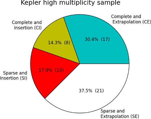
We show the distribution of Kepler high-multiplicity systems in the four subcategories based on BL13. The four subcategories are ‘complete and insertion (CI)’, ‘complete and extrapolation (CE)’, ‘sparse and insertion (SI)’ and ‘sparse and extrapolation (SE)’. The completeness of a system is measured by the spacing between two neighbouring planets. The insertion condition is such that if a system has fitting statistic with the TB relation worse than the Solar system, planet insertions are made to the system.
3 ANALYSIS
We revisited all 56 systems with the Q1–Q15 long-cadence Kepler public data (with more than 1000 d total time span), looking for additional periodic signals. First, we validated the detectability of all the known Kepler planetary candidates in these systems. We applied the Box Least Square Fitting (BLS) algorithm to the pre-filtered light curves. The pre-filtering processes included the removal of bad data points from the Kepler raw data (the |${\rm SAP\_FLUX}$|), the correction of safe modes and tweaks in the light curves, and the filtering of the systematic effects and stellar variations by a set of cosine functions with a minimum period of 1 d. We refer to Huang, Bakos & Hartman (2013) for more details about our pre-filtering technique. We then cross referenced our detected signals with the reported periods and epochs from the 2013 Kepler catalogue.
All the known transit signals in these systems have signal-to-noise ratios (SNRs) higher than 12 and dip significance (DSPs) higher than 8. These known transits from the systems were then removed from the raw (|${\rm SAP\_FLUX}$|) light curves with a window function 1.1 times wider than the reported transit duration from Kepler catalogue. The transits with high transit timing variations [TTVs; such as KOI-250 (Steffen et al. 2012a) and KOI-904 (Steffen et al. 2012b)] were removed by visual inspection of the light curves.
After the removal of all the known signals, the raw light curves were then cleaned by the same pre-filtering technique as above. We ran the BLS again on these light curves to ensure that the known signals have been fully removed. We selected the BLS peaks with the same threshold above. We also visually examined local maximums in the BLS spectrum within the predicted range of BL13 (regardless of their SNR). The selected peaks were then checked against our standard vetting procedures in Huang et al. (2013). Five new periodic planetary candidates were detected that passed our vetting procedures. We then derived the best-fitting parameters and their error bars of the vetted planetary candidates using the Markov Chain Monte Carlo algorithm.
We show the BLS spectrum of KOI-1952 in Fig. 2. The detected period has an SNR of 13.7 for the spectrum peak and a DSP of 9.0. There are three more peaks with comparable SNR in the spectrum, but their DSPs are all less than 8.
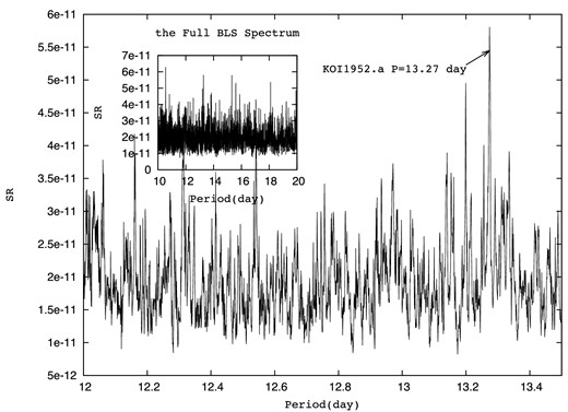
The BLS spectrum of KOI-1952 after the known transit signals removed. We zoomed in around the predicted period of the transit signal. The full spectrum is shown in the small window. All the other peaks of comparable height with the detected transit signal have much lower dip significance.
4 RESULTS AND DISCUSSION
4.1 Summary of detections
In this search among the 56 Kepler high-multiplicity systems, using SNR > 12 and DSP > 8 criteria, and visually inspecting the BLS spectrum in the predicted period range, we have not found the majority of the predicted planets from BL13. We found five of the predicted signals, and one periodic transit that was not predicted. We present the newly discovered transit signals in Fig. 3. The transit parameters are listed against the predicted periods in Table 1. We also list the known planetary candidates from Kepler team and their detection SNR and DSP in Table 1 as a comparison. Most of the detected signals indicate planets with size smaller than 2 R⊕. The detection SNR and DSP are on the low side of the overall population of Kepler candidates. However, the factor that they reside in multiple planet systems enhance their chances to be real planets (Lissauer et al. 2012).
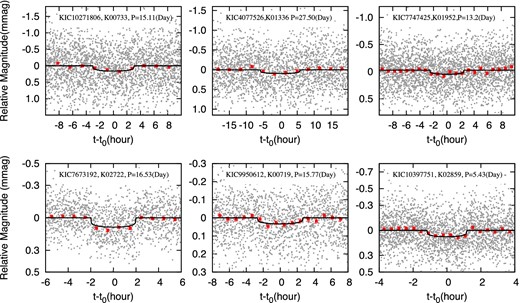
Folded light curves around the centre of transits t0 of the newly discovered planetary candidates from Kepler Q1-Q15 long-cadence data. The unbinned data are shown in grey dots, while the binned data are shown in red squares with the error bars representing the uncertainties in binned average. Superimposed are the best-fitting models of the transits. We note that the y-axis scales vary between subfigures.
Planet parameters.
| KIC | |$\chi ^2_\nu$|a | Originb | KOI | Period | Epoch(BJD−245 4000) | Rp/R⋆ | Rp/R⊕ | SNR | DSP |
|---|---|---|---|---|---|---|---|---|---|
| 9950612 | 1.35 | O | K00719.01 | 9.03 | 1004.014 | 0.023 | 1.64 | 1048 | 59 |
| O | K00719.02 | 28.12 | 979.913 | 0.0123 | 0.88 | 77 | 18 | ||
| O | K00719.03 | 45.90 | 999.538 | 0.0165 | 1.18 | 184 | 25 | ||
| O | K00719.04 | 4.159 | 966.784 | 0.0113 | 0.81 | 405 | 25 | ||
| N | K00719.a | |$15.7687_{-6}^{+5}$| | |$966.435_{-8}^{+10}$| | |$0.0059_{-10}^{+6}$| | 0.42 | 12 | 9 | ||
| I | K00719.I | 6.2 ± 0.6 | – | – | 0.6 | – | – | ||
| 0.49 | I | K00719.II | 14 ± 2 | – | – | 0.7 | – | – | |
| I | K00719.III | 20 ± 2 | – | – | 0.8 | – | – | ||
| E | K00719.IV | 66 ± 7 | – | – | 1.1 | – | – | ||
| 10271806 | 0.22 | O | K00733.01 | 5.925 020 | 1002.714 | 0.010 71 | 2.84 | 328 | 64 |
| O | K00733.02 | 11.349 30 | 967.318 | 0.010 93 | 2.47 | 195 | 24 | ||
| O | K00733.03 | 3.132 940 | 968.677 | 0.008 78 | 1.52 | 60 | 25 | ||
| O | K00733.04 | 18.643 90 | 974.620 | 0.009 93 | 2.55 | 13 | 14 | ||
| 4.06 | N | K00733.a c | |$15.111\,33_{-4}^{+3}$| | |$972.676_{-2}^{+2}$| | |$0.0113_{-4}^{+6}$| | 3.00 | 13 | 8 | |
| E | K00733.I d | 36 ± 4 | – | – | 2.8 | – | – | ||
| 4077526 | 1.06 | O | K01336.01 | 10.218 500 | 969.871 | 0.021 50 | 2.6 | 329 | 19 |
| O | K01336.02 | 15.573 800 | 965.438 | 0.021 69 | 2.6 | 177 | 11 | ||
| O | K01336.03 | 40.101 000 | 965.715 | 0.022 60 | 2.7 | 18 | 13 | ||
| O | K01336.04 | 4.458 250 | 967.387 | 0.014 31 | 1.7 | 31 | 9 | ||
| 1.35 | N | K01336.a | |$27.5066_{-1}^{+9}$| | |$977.882_{-3}^{+3}$| | |$0.0086_{-5}^{+6}$| | 1.04 | nan | nane | |
| I | K01336.I | 26 ± 3 | – | – | 2.4 | – | – | ||
| 0.19 | I | K01336.II | 6.8 ± 3 | – | – | 1.7 | – | – | |
| E | K01336.III | 61 ± 6 | – | – | 3.0 | – | – | ||
| 7747425 | 3.26 | O | K01952.01 | 8.010 350 | 1002.714 | 0.016 92 | 1.87 | 161 | 27 |
| O | K01952.02 | 27.665 000 | 976.876 | 0.018 67 | 2.06 | 14 | 17 | ||
| O | K01952.03 | 5.195 500 | 968.677 | 0.011 35 | 1.25 | 217 | 15 | ||
| O | K01952.04 | 42.469 900 | 979.305 | 0.018 21 | 2.01 | 30 | 13 | ||
| 0.64 | N | K01952.a | |$13.27242_{-1.3}^{+9}$| | |$973.014_{-4}^{+4}$| | |$0.0077_{-5}^{+9}$| | 0.85 | 14 | 9 | |
| I | K01952.I | 13 ± 2 | – | – | 1.5 | – | – | ||
| 0.01 | I | K01952.II | 19 ± 2 | – | – | 1.6 | – | – | |
| E | K01952.III | 65 ± 7 | – | – | 2.2 | – | – | ||
| 7673192 | 0.98 | O | K02722.01 | 6.124 820 | 967.935 | 0.010 93 | 1.47 | 215 | 28 |
| O | K02722.02 | 11.242 800 | 969.322 | 0.010 71 | 1.44 | 184 | 17 | ||
| O | K02722.03 | 4.028 710 | 966.775 | 0.008 78 | 1.18 | 17 | 15 | ||
| O | K02722.04 | 8.921 080 | 970.494 | 0.009 93 | 1.33 | 142 | 16 | ||
| N | K02722.a | |$16.5339_{-1}^{+1}$| | |$968.407_{-5}^{+7}$| | |$0.0086_{-5}^{+8}$| | 1.16 | 31 | 13 | ||
| E | K02722.I | 16.8 ± 1.0 | – | – | 2.8 | – | – | ||
| 10397751 | 1.69 | O | K02859.01 | 3.446 219 | 965.2274 | 0.0132 | 1.27 | 89 | 16 |
| O | K02859.02 | 2.005 396 | 966.2442 | 0.0074 | 0.72 | 99 | 13 | ||
| O | K02859.03 | 4.288 814 | 965.3824 | 0.0075 | 0.72 | 105 | 11 | ||
| O | K02859.04 | 2.905 106 | 965.5643 | 0.0086 | 0.83 | 150 | 10 | ||
| 1.07 | N | K02859.a | |$5.43105_{-4}^{+6}$| | |$967.41401_{-3}^{+5}$| | |$0.0079_{-6}^{+10}$| | 0.76 | 160 | 10 | |
| I | K02859.I | 2.41 ± 0.1 | – | – | 0.6 | – | – | ||
| E | K02859.II | 5.2 ± 0.3 | – | – | 0.8 | – | – |
aThe first value for every system is based the fitting before the insertion; the value next to the detected planet is based on the fitting including the detection; the value next to the predicted planet is based on the fitting including the prediction (but exclude the detection). A smaller |$\chi ^2_\nu$| indicates tighter fitting to the TB relation.
b‘O’ indicates KOI candidate from Kepler team. ‘N’ indicates new detections from this work. ‘I’ indicates inserted planets (predicted). ‘E’ indicates extrapolated planet (predicted).
cKOI number with letter indicates this is a new detection.
dKOI number with roman numbers indicates this is a predicted planet.
eThis candidate is found by identifying the BLS peaks visually around the predicted periods.
Details specific to each of the systems are spelled at below.
KOI-719 was predicted to host three ‘inserted’ planets and one ‘extrapolated’ planet. We found a planetary candidate with period of 15.77 d around the predicted period 14 ± 2 d. We do not see the rest of predicted planets in this system. Since KOI-719 is a small star (Rstar = 0.66 R⊙), this candidate is extremely small, with best-fitting radius similar to Jupiter's moon Ganymede, ∼0.42 R⊕. This new signal is around the 7:4 resonance of both its inner neighbour and its outer neighbour, reduces the system |$\chi ^2_\nu$| from 1.35 to 0.5.
KOI-1336 was predicted to host a 6.8 ± 3 d and another 26 ± 3 d ‘inserted’ planet. We recovered the latter at 27.5 d period. This signal is outside the 5:3 resonance with the inner planet (KOI-1336.02), and near the 2:3 resonance with the outer planet (KOI-1336.03). The |$\chi ^2_\nu$| of this system slightly increased with the insertion of this signal (from 1.06 to 1.35). If the 6.8 d planet exists (which we did not see in this search), this value would drop to 0.25. We failed to recover the ‘extrapolated’ 61 ± 6 d signal.
KOI-1952 was predicted to host two additional ‘inserted’ planets, with periods around 13 ± 2 d and 19 ± 2 d and an ‘extrapolated’ planet with a period of 65 ± 7 d. The detected signal matches well with the first prediction, and has a period of 13.3 d. This period is near the 3:2 resonance of KOI-1952.01, and near the 1:2 resonance of KOI-1952.02. We did not find any significant signal around the 19 d period. With the insertion of this transit signal, the |$\chi ^2_\nu$| of this system decreased from 3.25 to 0.64, following a tighter TB relation.
KOI-2722 was predicted to host an ‘extrapolated’ 16.8 ± 1 d transit. With the Q1–Q15 light curves, we recovered a new signal at a period of 16.5 d, which is also reported by Kepler team in the recent accumulated catalogue. This outer planetary candidate is near the 3:2 resonance with the previous outmost planetary candidates in the system. The next outer planetary candidate, predicted by BL13 around period of 24 ± 2 d, was not identified in our analysis.
KOI-2859 was predicted to host an ‘inserted’ planet with period around 2.41 ± 0.1 d and an ‘extrapolated’ planet with period around 5.2 ± 0.3 d. We only found the 5.43 d ‘extrapolated’ signal. It is not in tight resonances with any of the other planets in the system. The |$\chi ^2_\nu$| is improved to be 1.07.
We also have some detections that do not match the predictions. We found a new ‘inserted’ planetary candidate (with P = 15.1 d) in the KOI-733 system, which was predicted to host an ‘extrapolated’ planet with a period of 36 d. Although this system original fits better than solar, it was clarified as dynamically unpacked. Adding in this planet in the system will introduce the 4:3 resonance to the inner planet and the 4:5 resonance to the outer planet. However, this possible insertion will make the TB relation less tight; |$\chi ^2_\nu$| increased from 0.22 to 4.06.
We put these discoveries in the context of the four subcategories we stated in Section 2 (Table 2). We found three ‘inserted’ and one ‘extrapolated’ planetary candidates around the predicted periods in the 10 ‘sparse and insertion (SI)’ systems, and one ‘extrapolated’ planetary candidate around the predicted period in the 17 ‘complete and extrapolated (CE)’ systems. We did not find any transit signal within the error-bar of the predicted periods of the 8 ‘complete and insertion (CI)’ systems and 21 ‘sparse and extrapolated (SE)’ systems.
Detection summary.
| Catagorya | Num. predictionsb | Num. expectationsc | Num. detectionsd |
|---|---|---|---|
| SI | 10 (39) | |$7.8_{-1.7}^{+3.5}$| | 4 (4) |
| CI | 8 (20) | |$4.2_{-0.4}^{+1.2}$| | 0 (0) |
| CE | 17 (17) | |$2.2_{-0.6}^{+1.8}$| | 1 (1) |
| SE | 21 (21) | |$0.65_{-0.2}^{+0.8}$| | 0 (0) |
| Catagorya | Num. predictionsb | Num. expectationsc | Num. detectionsd |
|---|---|---|---|
| SI | 10 (39) | |$7.8_{-1.7}^{+3.5}$| | 4 (4) |
| CI | 8 (20) | |$4.2_{-0.4}^{+1.2}$| | 0 (0) |
| CE | 17 (17) | |$2.2_{-0.6}^{+1.8}$| | 1 (1) |
| SE | 21 (21) | |$0.65_{-0.2}^{+0.8}$| | 0 (0) |
a‘S’ (C) – the systems are sparse (complete); ‘I’(E) – the systems need (do not need) insertion. For detailed definition of each category, see Section 2.
bThe first number indicates the number of systems predicted, the second number indicates the total number of planets predicted in these systems.
cThe expected number of planets to be detected after accounting observational bias. We estimate this using the most likely Rayleigh distribution for inclination with |$\sigma _i = 1.8_{-0.8}^{+0.5}\,^{\circ }$| and the turnover power law for size correction. The upper bound and lower bound are 3σ limitations. We note that if using an inclination distribution suggested by Figueira et al. (2012), the expected number of predicted planets would be even higher.
dThe detected number of systems (planets) that match the predictions.
4.2 Detection bias analysis
We found that |$11_{-3}^{+12}$| out of 56 of the ‘extrapolated’ planets are expected to transit their host stars, while |$22_{-4}^{+10}$| out of 41 of the ‘inserted’ planets are expected to transit their host stars. We estimated the upper limit here using σi = 2| $_{.}^{\circ}$|3, and the lower limit with σi = 1| $_{.}^{\circ}$|0. The ‘extrapolated’ planets usually have longer periods, which are less likely to be detected than the ‘inserted’ planets. It would be interesting for future works to search for TTVs of the known planets in these systems to reveal potential non-transiting signals.
To explore the effect of a different size distribution, we also report the expected number of detections with the power-law distribution |$\frac{{\rm d}\,f(R)}{{\rm d}\, R} = kR^{-1}$| (constant occurrence rate in log space) in this radius range (R < 2 R⊕), as suggested by Petigura et al. (2013b). To avoid the singularity of integration with the plateau distribution at size 0, we set the lower limit of the planet size distribution to be 0.1 R⊕. One could of course argue that all the missing planets might as well be even smaller bodies than this, but it is out of the scope of this paper to discuss the region beyond our understandings. We found |$2.7_{-0.7}^{+2.2}$| extrapolated planets and |$7.3_{-1.2}^{+2.3}$| inserted planets are expected under this assumption.
We summarize the expected number of detection in the context of the four category of systems in Table 2, and compare them with detections. Generally speaking, our number of detections are below the expected lower limit of detections in most of the cases. Predictions in the ‘CI’ systems are ruled out at higher than 20σ level. Although BL13 claim majority (94 per cent) of the most complete systems tend to follow a tight TB relation, our findings indicate that those most complete systems that do not follow a tight TB relation could not be explained by missing planets.
4.3 Period ratio distributions
It is difficult to validate most of the predictions from the TB relations due to the uncertainty in the size distribution for small planets. However, we can use the period ratio distribution to examine the predicted planet population further, since there is no known strong bias against detections of planets in particular low-order period ratios. Steffen (2013) pointed out that there could be detection bias against adjacent period ratios that are larger than 5:1 or 6:1. In this analysis, we only focus on the region where adjacent period ratios are smaller than 3:1. We expect that the systems that do not need insertion (‘CE’ and ‘SE’) represent the underlying true period ratio distribution; while the planet systems needing insertion (‘CI’ and ‘SI’) should recover the same distribution after accounting for all the inserted planets. Our analysis here is independent of the number of predictions confirmed by our work.
We test the above expectation with these two populations in Fig. 4. The distribution of neighbouring period ratios for the ‘CE’ and ‘SE’ systems is shown with magenta; and the ‘CI’ and ‘SI’ systems with all their predicted inserted planets are shown in blue. For reference, we also plot in grey the distribution of ‘CI’ and ‘SI’ systems before the insertion. A striking feature is that the distribution of planetary systems after insertion looks significantly different from the systems that do not require insertion. We also performed a two-sample Kolmogorov–Smirnov statistic on the two populations, obtaining a KS p-value of 3 × 10⁻¹¹. It is unlikely that the ‘CI’ and ‘SI’ systems together with their inserted planets recovered the period ratio distribution suggested by the systems that do not require insertion. This indicates that some of the ‘insertion’ by BL13 might be problematic.
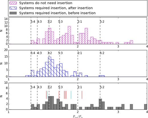
Histogram of period ratio between the neighbouring planet pairs in Kepler high-multiplicity samples. We present the systems that do not need insertion in magenta and hatched with ‘/’. The systems that required insertion, with all the inserted planets taken into account are shown in blue and hatched with ‘\’. We also shown the original (before insertion) period ratio distribution of systems needing insertion in grey. We marked out the position of the new discoveries in the bottom panel with vertical bars (red for ‘inserted’ planets and cyan for ‘extrapolated’ planets) for references.
By observing the detailed structures in the period ratio distribution, we found that systems following a tight TB relation (thus not needing insertion) is more likely to have period ratio around (wider to) the MMRs, such as 3:2, 5:3 and 2:1 resonances. Dynamic models (see Hansen & Murray 2013; Petrovich et al. 2013) can also reproduce these features. We note that the tail of the distribution at a period ratio higher than 3 is not statistically significant, the chance of having non-detected planets in these few sparse systems are not negligible (they follow the same size and inclination distribution arguments as in Section 4.1).
On the other hand, the systems that do not follow well a TB relation before their insertion have less pronounced peaks near the above MMRs. Including all the predicted ‘inserted’ planets, such that the systems can be optimally fitted by a tight TB relation, will preferentially add in (or modify) the period ratios close to the lowest order resonance in the original system. Therefore, the revised period ratio distribution according to the TB relation overpredicts the clustering around the 3:2 MMR and underpredicts the 2:1 MMR. It is hard to explain that most of the missing planets belong to the 3:2 MMR rather than the other MMRs by observation bias, unless there is a strong correlation between the period ratio of the adjacent planet and the size ratio of the adjacent planet, which is not seen in the previous study by Ciardi et al. (2013).
5 SUMMARY
The TB relation has been a recurrent theme in astronomy over the past two centuries. Investigations were all based on our Solar system – lacking other multiplanet systems. It is for the first time that validity of the TB relation can be tested on a statistically meaningful sample – thanks to hundreds of multiplanet discoveries made by the Kepler Space mission. By analysing the multiple systems and assuming that a general TB relation holds, BL13 predicted 141 new planets. We found only five of the predicted planets in the Kepler data. Some of the planets may be not finding because of small size or a non-transiting inclination angle. Nevertheless, even after taking these observational biases into account, the number of detected planets is still fewer than the 3σ lower limit of the expected planets from the prediction, hinting that it is questionable to apply such a law to all the extrasolar high-multiplicity systems.
We thank the anonymous referee for the insightful comments. We thank Zhou, G. for his comments on the draft and helpful discussions. Work by XCH and GB were supported by the NASA NNX13AJ15G and NSF AST1108638 grants.
See Kepler Object of Interest-Cumulative: http://exoplanetarchive.ipac.caltech.edu/cgi-bin/ExoTables/nph-exotbls?dataset=cumulative, also known as the 2013 Kepler catalogue.
The period of this planet has been corrected in the 2014 Kepler catalogue.
The dynamical spacing criteria for completeness of a planetary system are (a) all adjacent planet pairs have Δ values smaller than 10 if an additional planet is between each pair; (b) at least two adjacent planet pairs in the system have Δ values smaller than 10 if additional planet pairs are inserted.
Here, 1| $_{.}^{\circ}$|0 and 2| $_{.}^{\circ}$|3 are the 3σ lower and upper limit for the possible range of Rayleigh width. See fig. 6 of Fabrycky et al. (2012).
