


Abstract
High-mass binary stars are known to show an unexplained discrepancy between the dynamical masses of the individual components and those predicted by models. In this work, we study Sigma Scorpii, a double-lined spectroscopic binary system consisting of two B-type stars residing in an eccentric orbit. The more massive primary component is a β Cep-type pulsating variable star. Our analysis is based on a time series of some 1000 high-resolution spectra collected with the CORALIE spectrograph in 2006, 2007, and 2008. We use two different approaches to determine the orbital parameters of the star; the spectral disentangling technique is used to separate the spectral contributions of the individual components in the composite spectra. The non-LTE-based spectrum analysis of the disentangled spectra reveals two stars of similar spectral type and atmospheric chemical composition. Combined with the orbital inclination angle estimate found in the literature, our orbital elements allow a mass estimate of 14.7 ± 4.5 and 9.5 ± 2.9 M⊙ for the primary and secondary component, respectively. The primary component is found to pulsate in three independent modes, of which two are identified as fundamental and second overtone radial modes, while the third is an l = 1 non-radial mode. Seismic modelling of the pulsating component refines stellar parameters to 13.5|$^{+0.5}_{-1.4}$| and 8.7|$^{+0.6}_{-1.2}$| M⊙, and delivers radii of 8.95|$^{+0.43}_{-0.66}$| and 3.90|$^{+0.58}_{-0.36}$| R⊙ for the primary and secondary, respectively. The age of the system is estimated to be ∼12 Myr.
1 INTRODUCTION
Sigma Scorpii (σ Sco, HD 147165, HR 6084) is a quadruple system consisting of a close double-lined spectroscopic binary, and two other fainter stars at distances of about 0.4 and 20 arcsec (North et al. 2007, and references therein). The close pair consists of a B1 III β Cep-type variable star (hereafter called primary) and a B1 V companion (hereafter called secondary). The two stars reside in an eccentric orbit; the orbital period of the system is ∼33 d.
After the discovery of the radial velocity (RV) variations in the system by Slipher (1904), the star was subjected of numerous spectroscopic, photometric, and interferometric studies. Two spectroscopic studies by Levee (1952) and Struve, McNamara & Zebergs (1955) gave consistent results in the sense that both found variability intrinsic to the B1 giant star with the dominant period being about 0.25 d. Both studies reported about variability in the γ-velocity which was interpreted as evidence of a companion star. The orbital solution obtained by Levee (1952) and Struve et al. (1955) independently revealed an orbital period of about 33 d, though very different eccentricities of 0.2 and 0.36, respectively. In both cases, the dominant period of ∼0.25 d was attributed to stellar pulsations. Struve et al. (1955) additionally reported a period increase with the rate of 2.3 s century−1. Using the RVs collected by both authors, Fitch (1967) classified the star as a single-lined spectroscopic binary and reported an orbital solution in agreement with the findings by Struve et al. (1955), including a high eccentricity value of ∼0.4. Osaki (1971) argued, however, that the variability of the γ-velocity reported by Levee (1952) and Struve et al. (1955) is not necessarily connected to the existence of a stellar companion but might be related to non-radial pulsations.
Stars are expected to show slow changes in their dominant pulsation period in the course of the hydrogen exhaustion phase, but it is a matter of debate whether such an evolutionary effect is detectable. After the first report on the period change of the fundamental mode of the primary of σ Sco by Struve et al. (1955), a subsequent period decrease and increase was detected by Van Hoof (1966) and Sterken (1975), respectively. The latter study also reported on a periodicity of the observed variations with a period close to 23 yr.
Kubiak (1980) presented one of the first detailed periodicity studies for σ Sco based on the RVs obtained by Henroteau (1925), Levee (1952), and Struve et al. (1955). In total, a time series of 862 measurements has been analysed and revealed eight frequency peaks ranging in amplitude from 1 to 40 km s−1 (for the dominant mode). Two out of the eight frequencies, the dominant mode f1 = 4.051 11 d−1 (46.871 32 μHz) and f2 = 4.175 88 d−1 (48.314 95 μHz), were found to be independent modes whereas the other six frequencies appeared as their low-order combination terms (including harmonics). Based on the analysis of both photoelectric (taken in ubvy Stromgren system) and spectroscopic data, Kubiak & Seggewiss (1983) found non-radial pulsations to be the most reasonable explanation of the observed variability.
An extensive photometric study of the system was presented by Goossens et al. (1984) based on the observations collected by Van Hoof (1966) in the ultraviolet (UV), yellow (Y), and blue (B) light. The authors reported on the light variability in all three pass-bands with the same two dominant modes as found by Kubiak & Seggewiss (1983). On the other hand, the colour variations revealed only one dominant frequency f1 = 4.051 18 d−1 (46.872 15 μHz). The analysis performed by Goossens et al. (1984) on the RVs collected by Levee (1952) and Struve et al. (1955) appeared to be consistent with the analysis of the colour variations. The authors also found the dominant mode to be variable both in amplitude and phase with a period of ∼8.3 d, i.e. a quarter of the orbital period. Two models capable of representing the light variability intrinsic to the primary component were proposed: (i) two intrinsic pulsation modes with constant periods and amplitudes (in agreement with Struve et al. 1955 and Van Hoof 1966) and (ii) one intrinsic oscillation of which both the amplitude and the mean light curve are modulated by tidal action (supported by the results of the analysis of colour and RV variations).
Mathias et al. (1991) investigated the σ Sco system based on newly obtained time series of high-resolution, high-signal-to-noise ratio (S/N) échelle spectra. The authors reported the detection of the lines of the companion star in their spectra, and presented the orbital solution as summarized in Table 1. The Van Hoof effect that stands for a small phase lag of about 0.04P of the RV curve of the hydrogen lines behind all other spectral lines was detected in the system for the first time. Pigulski (1992) presented another study of the σ Sco system based on all photometric and spectroscopic data available at that time. The author determined the orbital parameters of the system as listed in Table 1 and investigated the O − C diagram of the main pulsation mode. The latter analysis revealed variability in the period of the dominant mode which Pigulski (1992) explained in terms of a superposition of the light-time effect due to a third body in the system and an evolutionary increase of the intrinsic pulsation period with a rate of 3 s century−1. These results are consistent with the early findings by Struve et al. (1955). Using the same data set as Pigulski (1992) did, Cugier & Boratyn (1992) performed a mode identification of the two dominant pulsation modes f1 = 4.051 21 d−1 (46.872 50 μHz) and f2 = 4.172 40 d−1 (48.274 67 μHz). The authors found that f1 is compatible with a radial mode whereas f2 is most probably an l = 2 mode. The identification for f1 was confirmed by Heynderickx, Waelkens & Smeyers (1994) later on, based on the information on the wavelength dependence of the photometric amplitudes.
Orbital solution for σ Sco as derived by Mathias, Gillet & Crowe (1991, indicated as M1991), Pigulski (1992, indicated as P1992), and North et al. (2007, indicated as N2007). Errors are given in parentheses in terms of last digits. Subscripts 1 and 2 refer to the primary and secondary component, respectively.
| Parameter | Unit | M1991 | P1992 | N2007 |
|---|---|---|---|---|
| P | d | 33.012(2) | 33.012 | 33.010(2) |
| K1 | km s−1 | 31.0(1.3) | 29.2(1.5) | |
| K2 | km s−1 | 40.3(7.2) | ||
| e | 0.44(11) | 0.40(4) | 0.3220(12) | |
| ω | deg | 299.0(10.0) | 287.0(6.0) | 283.0(5.0) |
| γ | km s−1 | 1.88(1.25) | 3.9(8) | |
| T0 | HJD (2434000+) | 889.4(7) | 888.0(4) | 889.0(1.0) |
| a1 sin i | (106) km | 13.0(2.4) | 12.2(6) | |
| a2 sin i | (106) km | 20.2(4.1) | ||
| f(M1) | M⊙ | 0.08(5) | 0.066(10) | |
| f(M2) | M⊙ | 0.30(18) |
North et al. (2007) derived the orbital solution and physical parameters of the σ Sco system based on interferometric data. The authors found a significantly lower eccentricity of about 0.32, whereas the other three orbital parameters (period P, time of periastron passage T0, and longitude of periastron ω) agreed within the errors with those reported by Mathias et al. (1991) and Pigulski (1992; cf. Table 1). Using the RV semi-amplitudes, K1 and K2, determined by Mathias et al. (1991), North et al. (2007) estimated the masses to be M1 = 18.4 ± 5.4 and M2 = 11.9 ± 3.1 M⊙, and assigned spectral types B1 III and B1 V to the primary and secondary components, respectively. Following the spectral type and luminosity class, an estimate of the effective temperature of the secondary of 25 400 ± 2000 K was presented for the first time.
Despite these efforts made by different research groups, no precise fundamental parameters for both binary components are available. For example, the effective temperature estimates for the β Cep pulsating primary component range from 21 880 (Beeckmans & Burger 1977) to 30 000 K (Theodossiou 1985, see table 4 in Vander Linden & Butler 1988 for an overview of the primary fundamental parameters estimates to which the values of Teff = 25 700 ± 1500 K and log g = 3.85 derived by Niemczura & Daszyńska-Daszkiewicz 2005 have to be added). On the other hand, only one rough estimate of the temperature of the secondary by North et al. (2007) is available in the literature. The log g of the primary is not well constrained either, ranging from 3.5 (Underhill et al. 1979) to 4.0 dex (Schild, Peterson & Oke 1971; Heasley, Wolff & Timonthy 1982). No estimate of this parameter exists for the secondary. Moreover, a possible influence of the large-amplitude (∼80 km s−1; Kubiak 1980) radial pulsation mode on the orbital solution has been ignored in all previous studies, which might have a significant impact on the determined orbital and physical parameters of the system. This motivated us to start this work, with the aim to determine precise orbital and stellar parameters of the system, evaluate atmospheric chemical composition and deduce the current evolutionary stage of both binary components, ideally from asteroseismic modelling.
We present our newly obtained high-quality spectroscopic data as well as describe the basic steps of the data reduction in Section 2. Section 3 is devoted to the orbital solution which we obtained by means of an iterative method. The orbital elements and the analysis of separated spectra obtained with the spectral disentangling (SPD) technique are presented in Section 4. System and physical parameters of σ Sco are discussed in Section 5. We present the results of the spectroscopic mode identification in Section 6. Stellar modelling is described in Section 7. The paper closes with a discussion and conclusions presented in Section 8.
2 OBSERVATIONS AND DATA REDUCTION
We obtained a time series of 1020 high-resolution, high-S/N spectra with the CORALIE spectrograph attached to the 1.2 m Euler Swiss Telescope (La Silla, Chile). The data were gathered during three consecutive years, in 2006, 2007, and 2008. The spectra have a resolving power of R = 50 000 and cover a 3000 Å wide wavelength range, from 381 to 681 nm. Table 2 gives the log of our spectroscopic observations and lists the period of observations (both calendar and Julian Dates) and the number of acquired spectra during the corresponding period.
List of the spectroscopic observations of σ Sco. JD is the Julian Date, N gives the number of spectra taken during the corresponding observational period.
| Time period | N | |
|---|---|---|
| Calendar date | JD (2 450 000+) | |
| 11.03–11.03.2006 | 3805.82–3805.87 | 7 |
| 14.03–18.03.2006 | 3808.78–3812.86 | 46 |
| 05.04–05.04.2006 | 3830.79–3830.91 | 17 |
| 08.04–09.04.2006 | 3833.77–3834.92 | 26 |
| 12.04–12.04.2006 | 3837.70–3837.85 | 19 |
| 31.05–31.05.2006 | 3886.59–3886.86 | 6 |
| 04.06–06.06.2006 | 3890.59–3892.62 | 6 |
| 08.06–08.06.2006 | 3894.56–3894.83 | 21 |
| 10.06–17.06.2006 | 3896.70–3903.83 | 134 |
| 27.07–30.07.2006 | 3944.49–3946.72 | 14 |
| 05.08–15.08.2006 | 3953.49–3962.62 | 326 |
| 19.03–23.03.2007 | 4178.90–4182.92 | 22 |
| 25.03–26.03.2007 | 4184.90–4185.92 | 8 |
| 30.03–31.03.2007 | 4189.91–4190.93 | 9 |
| 18.04–22.04.2007 | 4208.87–4212.95 | 92 |
| 25.04–26.04.2007 | 4215.88–4216.95 | 26 |
| 28.04–29.04.2007 | 4218.85–4219.94 | 34 |
| 22.07–28.07.2007 | 4303.57–4309.70 | 136 |
| 30.07–31.07.2007 | 4311.59–4312.59 | 41 |
| 13.06–15.06.2008 | 4630.54–4632.78 | 30 |
| Total number of spectra: | 1020 | |
The data reduction has been completed using a dedicated pipeline and included bias and stray-light subtraction, cosmic rays filtering, flat fielding, wavelength calibration by ThAr lamp, and order merging. The continuum normalization was done afterwards by fitting a (cubic) spline function through some tens of carefully selected continuum points. More information on the normalization procedure can be found in Pápics et al. (2012).
As it is mentioned in the Introduction, σ Sco is in fact a quadruple system with one of the components being a triple star. This three stellar component system consists of a double-lined spectroscopic binary (the one we study in this paper) and a 2.2 mag fainter tertiary at a distance of about 0.4 arcsec from the close pair. Despite this proximity of the third component, no signature of it could be detected in our composite spectra. Moreover, a compilation of the speckle interferometric observations of σ Sco presented by Pigulski (1992) shows that only a small part of the tertiary orbit was covered within ∼12 yr. Nather, Churms & Wild (1974) and Evans et al. (1986) suggested the orbital period of the order of 100–350 yr from the analysis of the lunar occultations of σ Sco. This means that the orbital period of the tertiary is much larger than the time base of our observations. As such, the third component does not affect our spectroscopic analysis of the close pair, and we neglect it in our study.
3 ORBITAL SOLUTION: ITERATIVE METHOD
In this section, we describe the way RVs of both components of σ Sco were determined from the composite spectra and present our first attempt to compute precise orbital solution by means of an iterative procedure.
3.1 Calculation of the RVs
The RVs of both binary components were computed based on the observed composite profiles of the Si iii 4552 Å spectral line. The observations were fitted with a superposition of two Gaussian profiles; the free parameters were RV, full width at half-maximum, and the strength for each of the two profiles. Fig. 1 illustrates an example of the double-Gaussian fit to one of the composite line profiles of the σ Sco binary. The derived RVs of both components are indicated by the vertical dotted lines; the fit itself is shown by the dashed line.
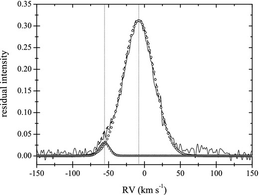
The composite profile of Si iii 4552 Å spectral line observed at JD 245 4311.6368 (solid line) with the best-fitting double-Gaussian profile overplotted (dashed line). The vertical dotted lines mark the derived RVs for both components. The individual Gaussians are shown by open circles and triangles for the primary and secondary, respectively.
Determination of the RVs of both stellar components was possible only for approximately a quarter of all the spectra we had at our disposal. In all other cases, the RVs of the secondary component could not be measured, lacking the detection of the companion's contribution in the observed composite spectra of the binary. The detection of the lines of the secondary, in most cases, was prevented by the large-amplitude spectral variability due to the radial pulsation mode of the primary component. This variability manifests itself in terms of large periodic shifts of the lines of the primary in velocity space, which means that the spectra taken at the same orbital phase look very different depending on the phase at which the pulsation mode of the primary is caught. After a careful inspection, we found that even those RVs of the secondary which we could measure from the composite profiles were significantly affected by the radial mode of the primary. Thus, we computed our orbital solution in a single-lined binary mode, relying on the RVs of the primary only. The RVs are shown in Fig. 2 along with the obtained orbital solution (see below).
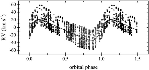
RVs of the pulsating primary of the σ Sco system (symbols) folded with the orbital period of 33.076 d (see text). Open circles, filled triangles, and stars refer to the data from 2006, 2007, and 2008, respectively. The best fit is shown with the solid line.
3.2 Orbital elements
For the calculation of the orbit of the primary component, we used a computer program that is based on the method of differential corrections to the orbital elements (see, e.g., Schlesinger 1910; Sterne 1941) and was written by one of us (HL). We optimized for the following six orbital elements simultaneously: the orbital period P, the time and the longitude of the periastron (T0 and ω, respectively), the semi-amplitude (K1) of the primary and gamma-velocity (γ) of the system, and the orbital eccentricity e. Fig. 2 illustrates the initial fit to the original data, where a large ‘RV-scatter’ is noticeable. This short-term variability is clearly intrinsic to the primary and is consistent with the radial pulsation mode with a frequency of ∼4.05 d−1 (46.86 μHz) reported in the previous studies. The derived orbital elements are listed in Table 3 (third column, indicated as ‘Original’). The elements differ significantly from those reported in Mathias et al. (1991) and North et al. (2007) who, in particular, found a significantly shorter orbital period and higher semi-amplitude of the primary, as well as significantly different γ-velocity and eccentricity of the system.
Orbital elements computed based on the RVs of the primary component. The two solutions are based on the original and the pre-whitened data sets (see text for details). Errors are given in parentheses in terms of last digits.
| Data set | |||
|---|---|---|---|
| Parameter | Unit | Original | Pre-whitened |
| P | d | 33.076(64) | 33.016(12) |
| K1 | km s−1 | 26.89(1.08) | 30.14(35) |
| e | 0.359(187) | 0.333(61) | |
| ω | deg | 272.7(6.6) | 281.4(1.6) |
| T0 | HJD (2434000+) | 881.4(3.8) | 885.8(1.0) |
| γ | km s−1 | −8.80(86) | −1.52(25) |
| rms | km s−1 | 16.7614 | 1.8556 |
Apparently, one needs to get rid of the large-amplitude intrinsic variability of the primary component to obtain a reliable orbital solution. One way to minimize the influence of the pulsations on the orbital solution is to introduce an iterative procedure which comprises of three basic steps: (i) calculation of the orbital solution and subtracting it from the original data set; (ii) searching for the periodicities in the obtained residuals; and (iii) subtracting the pulsation signal from the original data set and re-calculating the orbital solution. Our further analysis in this section is based on such a procedure which is repeated until no significant changes in the derived orbital elements and extracted frequencies occur anymore.
We used the period04 program (Lenz & Breger 2005) to search for the periodocities in the residuals. The decision on the significance of the extracted frequencies was made according to the significance level of S/N = 4.0 proposed by Breger et al. (1993) for ground-based data. The noise level was computed from a 3 d−1 box after pre-whitening the frequency peak in question. Table 4 lists all frequencies detected in our data assuming the stop criterion mentioned above. To verify our solution at each pre-whitening step, the corresponding residuals were compared to the previous data set from which the frequency in question has been subtracted. We found that the first four frequencies listed in Table 4 comprise the major part of the short-term variability present in the RVs of the primary of σ Sco. A further pre-whitening of the data from frequencies f5 and f6 leads to only a marginal improvement of the solution, by ∼0.15 km s−1 in terms of the rms. Our final orbital solution obtained after pre-whitening the six frequencies listed in Table 4 is given in the last column of Table 3; the quality of the fit is illustrated in Fig. 3. Frequencies f1, f3, and f5 have already been reported in several previous studies (see, e.g., Kubiak 1980; Jerzykiewicz & Sterken 1984; Cugier & Boratyn 1992), two frequencies, f2 and f4, appear to be the second and the third harmonics of the dominant mode, respectively, and frequency f6 is a new detection pending an independent confirmation. Using the inclination angle reported by North et al. (2007) and our estimates of the radius of the primary (cf. Section 5), we find that f6 is by ∼0.3 d−1 larger than the expected rotational frequency of this star.
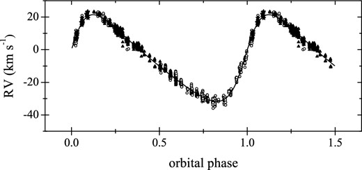
RVs of the primary of σ Sco after pre-whitening from six frequencies listed in Table 4. Open circles, filled triangles, and stars refer to the data from 2006, 2007, and 2008, respectively. The solid line shows the final orbital solution; the corresponding orbital elements are given in Table 3 (fourth column, indicated as ‘Pre-whitened’).
Frequencies found in the combined (residual) data set from 2006, 2007, and 2008. The frequency uncertainties are given by the Rayleigh limit which amounts to 0.0019 d−1 (0.0219 μHz). The amplitude errors are given in parentheses in terms of last digits.
| fi | Frequency | Amplitude | S/N | |
|---|---|---|---|---|
| (d−1) | (μHz) | (km s−1) | ||
| f1 | 4.0515 | 46.8759 | 23.6(1) | 144.8 |
| f2 = 2f1 | 8.1030 | 93.7517 | 2.0(5) | 12.4 |
| f3 | 4.1726 | 48.2770 | 1.4(1) | 9.2 |
| f4 = 3f1 | 12.1521 | 140.5998 | 1.1(2) | 7.9 |
| f5 | 5.9706 | 69.0201 | 1.0(2) | 5.5 |
| f6 | 0.5003 | 5.7885 | 0.7(2) | 4.1 |
Evolution of the amplitudes of the two dominant modes and harmonics of the radial mode through years 2006–2008. The amplitude errors are given in parentheses in terms of last digits.
| fi | Amplitude (km s−1) | ||
|---|---|---|---|
| 2006 | 2007 | 2008 | |
| f1 | 23.6(12) | 22.1(3) | 20.7(4) |
| f2 = 2f1 | 2.1(6) | 2.0(6) | 1.7(7) |
| f3 | 1.7(3) | 1.5(3) | 1.4(4) |
| f4 = 3f1 | 1.3(3) | 1.1(4) | 0.9(5) |
| fi | Amplitude (km s−1) | ||
|---|---|---|---|
| 2006 | 2007 | 2008 | |
| f1 | 23.6(12) | 22.1(3) | 20.7(4) |
| f2 = 2f1 | 2.1(6) | 2.0(6) | 1.7(7) |
| f3 | 1.7(3) | 1.5(3) | 1.4(4) |
| f4 = 3f1 | 1.3(3) | 1.1(4) | 0.9(5) |
In order to check for the stability of the frequencies and their amplitudes in time, we analysed the data sets from individual years separately. Given that the data subsets from 2007 and 2008 are shorter and contain less measurements than the one from 2006, it is not surprising that only the dominant mode at ∼4.05 d−1 (46.86 μHz) and its harmonics, and the mode at f3 ≃ 4.17 d−1 (48.25 μHz) could be detected in the corresponding data subsets. Our analysis revealed a small decrease of about 6 × 10⁻⁵ d−1 (7 × 10⁻⁴ μHz) of the frequency of the dominant mode between the years 2006 and 2007, which is two orders of magnitude smaller than the actual frequency resolution. The frequency resolution for the data taken in 2008 is too low to draw firm conclusions on the period increase/decrease during this season. A small but significant amplitude decrease of the two dominant modes and harmonics of the radial mode was also detected through the years 2006–2008 (see Table 5). This is consistent with the recent study by Handler (2014) who also reported a pulsation amplitude decrease in the primary of σ Sco, but at a larger rate. The short time base of our observations prevents us from drawing any firm conclusions with respect to the physical cause of the detected amplitude decrease. Finally, we note that the frequency of the dominant mode of 4.0515 d−1 (46.8759 μHz) detected by us from the combined data set is different from the one of 4.0512 d−1 (46.8724 μHz) reported by Pigulski (1992). This difference is still an order of magnitude smaller than provided by the frequency resolution of our data to conclude on any period changes of the dominant oscillation mode.
4 SPECTRAL DISENTANGLING
The orbital solution obtained in Section 3 is not perfect but provides a good starting point for the analysis with more sophisticated methods like the SPD technique. In the method of spd, as introduced by Simon & Sturm (1994), one simultaneously solves for the individual spectra of stellar components of a multiple system and a set of the orbital elements. Hadrava (1995) suggested an implementation of the technique in Fourier space, which significantly decreases the computation time. In this work, we apply the spd technique in Fourier space as implemented in the fdbinary code (Ilijic et al. 2004).
4.1 Orbital solution
All existing Fourier-based spd codes (including fdbinary) assume binarity to be the only cause of the line profile variations detected in the spectra. This implies that individual stellar components of a binary are supposed to be intrinsically non-variable, making the application of the method to our original data set impossible.
Our first attempt to solve the problem with the intrinsically variable primary component of σ Sco was to bin the original spectra with the orbital period determined in Section 3. From a set of experiments, we have found 50 orbital phase bins (corresponding to an orbital phase bin width of 0.02) to be the optimal choice: this minimized the number of orbital phase gaps, on the one hand, and provided sufficient pulsation phase coverage in each bin, on the other hand. A selection of a larger/smaller bin width is associated with additional uncertainties due to the displacement of the lines of the secondary within a given bin, and due to an increased number of orbital phase gaps, respectively. If the spectra were uniformly distributed with the (dominant) pulsation period of the primary in each orbital phase bin, one would expect the effect of the stellar oscillations to cancel out, providing us with a data set well suitable for orbit determination and SPD. In reality, the spectra do not show such a uniform distribution with the pulsation phase, and the spd technique delivers unreliable results. We attempted to solve the problem by selecting only those spectra that deviated from the mean spectrum of the corresponding bin in RV by less than 2 km s−1. At this point, we still assume that the mean spectrum in each bin represents a zero pulsation phase (unperturbed profile). Although this is not the case, our tight selection criterion of 2 km s−1 for the individual spectra led to the remarkable suppression of the amplitude of the dominant pulsation mode, compared to the binning procedure alone. This selection resulted in 131 useful spectra out of 1020 that we had in total. The value of 2 km s−1 is not a random choice but was selected based on a set of experiments. In particular, we aimed to reduce the influence of the dominant radial mode on the orbital solution as much as possible, and, on the other hand, to have enough spectra to provide sufficient orbital phase coverage, which would make the determination of precise orbital elements possible. For the calculation of the orbital elements, we used five spectral intervals centred at the C ii 4267 Å, He i 4471 Å, He i 4713 Å, He i 5015 Å, and He i 5047 Å lines. The orbital solution obtained based on the selection of spectra described above is indicated as ‘Solution 1’ in Table 6; the corresponding orbital elements are listed in the third column. We fixed the period to the value obtained in Section 3, all other parameters were allowed to be free. The derived values of eccentricity and time of the periastron passage are consistent with those obtained from the iterative approach (cf. Table 3), whereas the longitude of the periastron and, particularly, the semi-amplitude K1 differ significantly. After a careful inspection of the disentangled spectra in the five spectral regions mentioned above, it became clear that the solution still suffers from the large-amplitude-dominant pulsation mode of the primary component. In particular, some weak ‘absorption’ features showed up in the outer wings of the photospheric stellar lines. The positions and regularity of these features suggest that they are artificial and have nothing to do with real absorption in the photosphere of either of the binary components. To solve the problem, we reduced our set of 131 spectra even further, by tightening the selection criterion from 2 to 1 km s−1. This selection gave us 30 spectra that were finally used for the SPD. The bottleneck of such selection is that the spectra do not provide good enough orbital phase coverage, in the sense that the regions around the minimum and maximum RV are badly covered. This makes the determination of the eccentricity impossible; thus, we decided to fix it to the value obtained from the previous solution that was obtained based on the selection of 131 spectra. The remaining four orbital elements, semi-amplitudes K1 and K2, longitude of the periastron ω, and the time of the periastron passage T0, were set as free parameters. The orbital solution obtained this way is indicated as ‘Solution 1’ in Table 6; the corresponding orbital elements are given in the fourth column.
Orbital solutions obtained by means of the SPD technique based on two different sets of spectra (see text for details). Errors of measurement are 1σ standard deviations and are given in parentheses in terms of last digits.
| Data set | |||
|---|---|---|---|
| Parameter | Unit | Orbit | Orbit+Spectra |
| Solution 1 | |||
| P | d | 33.016(12)a | 33.016(12)a |
| K1 | km s−1 | 24.32(12) | 25.31(13) |
| K2 | km s−1 | 51.03(93) | 49.70(50) |
| e | 0.334(2) | 0.334(2)b | |
| ω | deg | 289.0(8) | 282.0(5) |
| T0 | HJD (2434000+) | 885.17(6) | 884.63(5) |
| Solution 2 | |||
| P | d | 33.016(12)a | 33.016(12)a |
| K1 | km s−1 | 30.14(35)a | 30.14(35)a |
| K2 | km s−1 | 41.86(1.25) | 47.01(98) |
| e | 0.383(8) | 0.383(8)b | |
| ω | deg | 294.4(1.7) | 288.1(8) |
| T0 | HJD (2434000+) | 886.42(12) | 886.11(4) |
aFixed to the value obtained in Section 3.
bFixed to the value from solution ‘Orbit’.
The disentangled spectra obtained from our Solution 1 were used for a detailed spectrum analysis by means of the methods outlined in Section 4.2. The analysis showed that the obtained orbital solution assumes a too small contribution of the secondary component to the total light of the system. In the result, the disentangled spectrum of the secondary shows an unreliably high abundance of oxygen: we detected an overabundace above 1 dex compared to the standard cosmic abundances reported in Nieva & Przybilla (2012). Such large oxygen enrichment is not predicted theoretically and has not been previously detected in any high-mass star. Moreover, Morel (2009) shows that OB stars tend to show slightly sub- or at most solar oxygen abundances. This led us to think that the obtained orbital solution is not reliable and this, in particular, concerns the K1 semi-amplitude of the primary component. Indeed, the value of ∼25 km s−1 that we obtained is very close to the RV semi-amplitude of the primary's dominant pulsation mode (cf. Table 4), and is significantly lower than the value derived in Section 3.2 and reported in Mathias et al. (1991) and Pigulski (1992), for example.
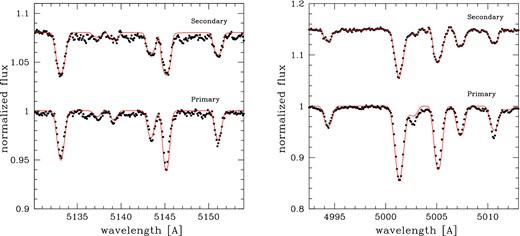
In the next step, we fixed the orbital period and RV semi-amplitude of the primary to the values derived in Section 3.2, and re-computed our orbital solution and the disentangled spectra. This was also done in two steps: (i) using the set of 131 spectra and allowing eccentricity to be one of the free parameters and (ii) fixing additionally the eccentricity and fine-tuning K2, ω, and T0 based on the reduced set of the 30 observed spectra. Both steps are depicted in Table 6 as ‘Solution 2’, where the fourth column lists the orbital elements that we consider as the final ones. Except for the value of ω, this orbital solution agrees within the error bars with our preliminary solution from Table 3. These orbital elements were used to compute the disentangled spectra of both stars; a small part of the raw spectra non-corrected for the individual light contributions is illustrated in Fig. 4. The spectrum of the primary was vertically shifted for better visibility. From visual inspection of the spectra, it is obvious that both stars are of similar spectral type but have (slightly) different rotational velocities. The detailed spectrum analysis of both stars is outlined in the next section and includes the estimation of their fundamental parameters and atmospheric chemical composition.
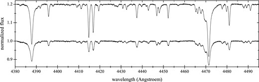
A portion of the raw, non-corrected for the individual light contributions disentangled spectra of both components of the σ Sco binary. The spectrum of the primary was vertically shifted by a constant value for visibility purposes.
4.2 Spectrum analysis of both binary components
In the case of eclipsing binaries, a combination of high-resolution spectroscopic data and a SPD technique allows the estimation of the effective temperatures and surface gravities as well as chemical composition of individual binary components to a very high precision (see, e.g., Pavlovskib & Hensberge 2005; Hareter et al. 2008; Pavlovski & Southworth 2009; Tkachenko, Lehmann & Mkrtichian 2009, 2010). Though the accuracy that is reached in the parameters derived from spectroscopy for the components of non-eclipsing systems is comparable to the one achieved for single stars, it is still significantly higher than the accuracy expected from the analysis of broad-band photometric data, for example.
Before the disentangled spectra can be analysed to determine properties of stars, they have to be renormalized to the individual continua according to the light ratio of the stars. This important parameter can be accurately determined for eclipsing binaries from photometric data (see, e.g., Pavlovski et al. 2009; Tkachenko et al. 2012; Debosscher et al. 2013; Hambleton et al. 2013; Lehmann et al. 2013). When a binary star is not eclipsing or no photometric data are available in the eclipses, the light ratio is set as a free parameter and is determined simultaneously with the fundamental parameters of the components from the disentangled spectra (the so-called constrained fitting; Tamajo, Pavlovski & Southworth 2011). The fundamental parameters of both stars were determined by fitting the disentangled spectra to a grid of synthetic spectra. The grid was computed based on the so-called hybrid approach, that is using LTE-based atmosphere models calculated with the atlas9 code (Kurucz 1993) and non-LTE spectral synthesis by means of the detail (Butler 1984) and surface (Giddings 1981) codes. Justification of such approach is discussed in Nieva & Przybilla (2007). The procedure we used to estimate the fundamental parameters and chemical composition of both components of the σ Sco system is outlined in detail in Tamajo et al. (2011) and Tkachenko et al. (2014).
Table 7 lists the atmospheric parameters and individual abundances of both stellar components of the σ Sco system; the quality of the fit to a set of carbon and nitrogen lines is shown in Fig. 5. The errors in the parameters and abundances are 3σ levels, with σ the standard deviations of the mean. The way we did the selection of the spectra suitable for the SPD (see Section 4.1 for details) was such as to use the spectra representative of the equilibrium stage of the primary component with respect to its dominant radial pulsation mode. Consequently, the fundamental parameters of the primary listed in Table 7 are valid for the equilibrium state of the primary. Note that Morel et al. (2006) investigated the effect of taking spectra at minimum and maximum radius for the large-amplitude radial β Cep pulsator ξ1 CMa and found a range in Teff and log g equal to 1000 K and 0.1 dex, respectively. The amplitude of the radial mode of σ Sco is somewhat larger than the one of ξ1 CMa, so we expect the same range to apply here. For this reason, we carefully selected spectra at the equilibrium phase of the primary to deduce the fundamental parameters. The binary components are found to have similar spectral types and chemical composition, but differ in luminosity class. For the majority of the elements, the derived abundances agree within 3σ error bars with the cosmic abundance standard (CAS) determined by Nieva & Przybilla (2012) from the analysis of B-type stars in OB associations and for field stars in the solar neighbourhood. An exception is the carbon abundance found in the secondary which is at ∼0.2 dex lower level than the CAS value.
Best fit (lines) to a set of carbon (left) and nitrogen (right) lines in the spectra of both components of the σ Sco binary system.
Atmospheric parameters and individual abundances of both components of the σ Sco system. Abundances are expressed relative to log N(H) = 12.0. Cosmic abundance standard (CAS) is taken from Nieva & Przybilla (2012). Error bars are expressed in terms of a 3σ level.
| Parameter | Unit | Primary | Secondary | |
|---|---|---|---|---|
| Atmospheric parameters | ||||
| Teff | K | 25 200 ± 1 500 | 25 000 ± 2 400 | |
| log g | dex | 3.68 ± 0.15 | 4.16 ± 0.15 | |
| vsin i | km s−1 | 31.5 ± 4.5 | 43.0 ± 4.5 | |
| vturb | km s−1 | 14.0 ± 3.0 | 4.0 ± 3.0 | |
| Individual abundances | ||||
| Elem. | Unit | Primary | Secondary | CAS |
| He | 10.94 ± 0.24 | >10.70 | 10.99 ± 0.01 | |
| C | 8.20 ± 0.12 | 8.11 ± 0.12 | 8.33 ± 0.04 | |
| N | 7.68 ± 0.09 | 7.62 ± 0.21 | 7.79 ± 0.04 | |
| O | dex | 8.76 ± 0.21 | 8.79 ± 0.24 | 8.76 ± 0.05 |
| Si | 7.43 ± 0.24 | 7.43 ± 0.36 | 7.50 ± 0.05 | |
| Mg | 7.40 ± 0.30 | 7.35 ± 0.36 | 7.56 ± 0.05 | |
| Al | 6.07 ± 0.15 | 6.03 ± 0.15 | ||
We present a lower limit for the atmospheric helium abundance of the secondary component only. Several strong He i lines that were used to derive the helium content for this star suggested an abundance of ∼10.70 dex, which is significantly lower than the CAS value. On the other hand, the abundance inferred from the He ii line at λ 4686 Å is consistent with the CAS value. This discrepancy between the abundances inferred from He i and He ii lines cannot be explained by an erroneous effective temperature for the secondary; however, the temperature of this star is well constrained by the visibility of He ii line at λ 4686 Å and the absence of two other He ii lines at λ 4200 and λ 4541 Å in its spectrum. Though a temperature change could account for low helium abundance obtained from the lines of neutral atoms of this element, it also greatly affects the visibility of He ii lines and the quality of the fit of metal and hydrogen lines in the spectrum of this star. Thus, we conclude that the strong He i lines present in the spectrum of the secondary still suffer from the large-amplitude oscillations of the primary in the composite spectra, and the helium abundance derived by us for the secondary component can only be considered as a lower limit.
5 SYSTEM AND PHYSICAL PARAMETERS OF σ SCO
The fact that σ Sco is not an eclipsing binary withholds us from measuring the orbital inclination angle and thus the masses of the individual stellar components. We use the orbital inclination angle determined by North et al. (2007) from interferometry to estimate the physical parameters of both components of the σ Sco system. We point out that North et al. (2007) did not take into account the pulsations of the primary in their analysis.
Table 8 lists the system and physical parameters of σ Sco. The errors in the parameters arising from the uncertainties in the orbital elements were computed by repeating the calculations after varying the elements within their 1σ uncertainty levels. Our masses are lower than those reported by North et al. (2007), although both estimates agree within the error bars, which reveal rather bad precisions of ∼30 per cent for the masses of both stars. The total mass of the system of 30.3 ± 9.0 M⊙ presented by North et al. (2007) is about 25 per cent larger than the total mass derived in this study. This is primarily due to the large differences in the assumed semi-amplitude of the secondary component and the eccentricity of the system. Given the large error bars, the mass of the primary component of 14.7 ± 4.5 M⊙ derived by us is in agreement with the majority of members from the catalogue of Galactic β Cep stars (Stankov & Handler 2005), where the mass distribution was found to peak at 12 M⊙.
System and physical parameters of the σ Sco binary.
| Parameter | Unit | Primary | Secondary |
|---|---|---|---|
| Orbital inclinationa (i) | deg | 21.8 ± 2.3|$\hphantom{0}$| | |
| Semimajor axis (a) | au | 0.583 ± 0.064 | |
| Ang. semimajor axisa (a″) | mas | 3.62 ± 0.06 | |
| Ang. diametera (θ) | mas | 0.67 ± 0.03 | 0.34 ± 0.04 |
| Mass (m) | M⊙ | 14.7 ± 4.5 | 9.5 ± 2.9 |
| Radius (R) | R⊙ | 9.2 ± 1.9 | 4.2 ± 1.0 |
| 11.3 ± 1.6b | 5.8 ± 1.2b | ||
| Luminosity (log(L)) | L⊙ | 4.49 ± 0.24 | 3.80 ± 0.26 |
| 4.67 ± 0.17b | 4.07 ± 0.26b | ||
aTaken from North et al. (2007).
bComputed from angular diameters.
The radii of the components derived from the masses and gravities, and from the angular diameters of the stars, differ by about 1.9 and 1.6 R⊙ for the primary and secondary, respectively. This difference is within the quoted error bars. North et al. (2007) reported the radius of 12.7 ± 1.8 R⊙ for the pulsating primary component and adopted the radius of 6.4 R⊙ for the secondary from its spectral classification. The difference between our radius of the primary determined from its angular diameter and the North et al. (2007) value is due to the difference in the semimajor axis of the system (see above). In Section 7, we perform a detailed asteroseismic modelling of the primary component of σ Sco to verify the determined masses and radii of both binary components.
6 SPECTROSCOPIC MODE IDENTIFICATION
In this section, we describe the results of the spectroscopic mode identification for the primary of σ Sco. We make use of the orbital solution and the disentangled spectrum of the secondary obtained in Section 4.1 to subtract the contribution of the secondary component from the observed, composite spectra and to shift the residual profiles to the reference frame of the primary.
For the extraction of the individual frequencies from both RVs and line profiles, we used the discrete Fourier-transform (DFT) and the consecutive pre-whitening procedure as implemented in the famias package (Zima 2008). The DFT was computed up to the Nyquist frequency of the data set, and similar to the results presented in Section 3.2, no significant contribution was found in the high-frequency domain. At each step of the pre-whitening, we optimized the amplitudes and phases of the individual peaks whereas the frequency values were kept fixed. We restricted our analysis to the Si iii 4552 Å spectral line which is known to be sensitive to stellar oscillations in hot stars (Aerts & De Cat 2003).
Both the Fourier-parameter fit (FPF; Zima et al. 2006) and the moment (Aerts, de Pauw & Waelkens 1992) methods give results consistent with those presented in Section 3.2. Three independent modes with frequencies f1 = 4.0513, f3 = 4.1727, and f5 = 5.9702 d−1 were unambiguously detected with both methods, while the frequency f6 = 0.4997 d−1 could be detected in the RVs only and with low significance level (S/N = 3.8). In addition, the orbital frequency and the second and the third harmonics of the dominant radial mode have been detected with both diagnostics.
In the next step, we used all our 1020 spectroscopic measurements to identify two out of three detected frequencies in terms of l and m quantum numbers. We fixed l = 0 for the f1 = 4.0513 d−1 mode, according to previous studies (e.g. Cugier & Boratyn 1992; Heynderickx 1994) and characteristic for radial modes displacements of the oscillation-sensitive spectral lines in the course of the pulsation cycle. This allows us to limit the parameter range to two independent modes during mode identification and to speed up the calculations.
Similar to the frequency analysis, the mode identification is performed using two different approaches, the FPF and the moment methods. Both rely on the calculation of the synthetic profiles but use different observables to deliver the identification of the individual pulsation modes. In the FPF method, the observed Fourier parameters zero-point, amplitude, and phase across the line profile are compared to the theoretical values, while in the moment method, one relies on the integrals of the line profile (Zima 2008). To provide sufficient spatial resolution, we divide the stellar surface into 10 000 segments. The required fundamental parameters like mass, radius, etc. were set according to our best-fitting model presented in Table 9 (see also Section 7 for details).
Parameters of the three best-fitting stellar evolution models. See text for details.
| Model | Temperature (Teff) | Gravity (log g) | Mass (M) | Radius (R) | Overshoot (fov) | Hydrogen content (Xc) | Age | Reduced |
|---|---|---|---|---|---|---|---|---|
| (K) | (dex) | (M⊙) | (R⊙) | Hp | mass fraction | (Myr) | χ2 | |
| 1 | 23 945|$^{+500}_{-990}$| | 3.67|$^{+0.01}_{-0.03}$| | 13.5|$^{+0.5}_{-1.4}$| | 8.95|$^{+0.43}_{-0.66}$| | 0.000+0.015 | 0.14|$^{+0.05}_{-0.01}$| | 12.1|$^{+2.0}_{-1.0}$| | 4.033 |
| 2 | 23 430|$^{+1020}_{-580}$| | 3.66|$^{+0.02}_{-0.02}$| | 13.0|$^{+1.0}_{-0.9}$| | 8.85|$^{+0.53}_{-0.56}$| | 0.000+0.015 | 0.13+0.06 | 12.9|$^{+1.2}_{-1.8}$| | 10.980 |
| 3 | 22 855+1600 | 3.64+0.04 | 12.1+1.9 | 8.70+0.35 | 0.015−0.015 | 0.19−0.06 | 13.6|$^{+0.5}_{-2.5}$| | 11.496 |
The moment method delivers unambiguous mode identifications for f3 and f5 as being (l, m) = (1,1) and a radial modes, respectively. Our 10 best solutions provide the same identification for these two modes but disagree on the inclination angle of the rotation axis to the line of sight and the amplitude of the f5 mode. The inclination angle varies between 17° and 32°, and we cannot distinguish between different solutions due to rather small changes in the χ2 value. Given the range in the inclination angle, the primary of σ Sco has equatorial rotation velocity between 60 and 110 km s−1. Using the mass and radius derived in the next section, we find the primary to rotate between 13.5 and 25 per cent of its break-up velocity. The orbital inclination angle of 21| $_{.}^{\circ}$|8 ± 2| $_{.}^{\circ}$|3 reported by North et al. (2007) is within the range we derived for the inclination angle of the rotation axis of the primary. This suggests spin–orbit alignment or at most slight misalignment for the primary component of the σ Sco system.
The results of the mode identification obtained with the FPF method are less satisfactory, however. A variety of solutions with nearly the same goodness of the fit was obtained. For both fitted modes, f3 and f5, the spherical degree l was found to range between 0 and 3, with a slight preference for f3 being l = 1 or 2 mode. It is well known that the moment method is better suitable for slow to moderate rotators, while sufficiently large rotational broadening of the lines is required for the FPF method to work properly. The limitations we encountered in using the FPF technique for the mode identification is probably due to the insufficient rotational broadening of the lines of the primary.
7 ASTEROSEISMIC MODELLING
Asteroseismic modelling of massive stars is done by adapting a forward modelling approach for frequency matching, starting from a set of models in the spectroscopic error box (Teff, log g) of the star (Aerts, Christensen-Dalsgaard & Kurtz 2010, Chapter 7). We use the mesa stellar structure and evolution code developed by Paxton et al. (2011, 2013) to compute non-rotating models. This is justified in view of the relatively modest rotation of less than a quarter of the critical velocity. The initial abundance fractions (X, Y, Z) = (0.710, 0.276, 0.014) are those from Nieva & Przybilla (2012), in agreement with the spectroscopic findings (cf. Section 4). Convective core overshoot is described in exponentially decaying prescription of Herwig (2000). The Ledoux criterion is used in the convection treatment. The opal opacity tables of Iglesias & Rogers (1996) and mesa equation-of-state are used.
We screened the mass range from 10 up to 20 M⊙ to interpret the pulsations of the primary component of σ Sco. The central hydrogen content (Xc) and the overshooting parameter (fov) were also varied in the ranges from 0.7 to 0.0 and 0.0 to 0.03, respectively, which corresponds with our step-wise overshoot parameter of αov ϵ [0.0,0.3]Hp. All models fitting the observed spectroscopic values of Teff and log g within 5σ have been selected. This selection resulted in some 28 000 evolutionary models whose p- and g-mode eigenfrequencies for mode degrees l = 0 to 3 have been calculated in the adiabatic approximation with the gyre stellar oscillation code (Townsend & Teitler 2013). The theoretical frequencies were compared with the three observed dominant modes of the primary of σ Sco (f1, f3, and f5; cf. Table 4). The best-fitting model was selected using a χ2 criterion. Fig. 6 (light grey dots in the top and middle panels) illustrates χ2 distributions for six stellar parameters (from top-left to middle-right: effective temperature, surface gravity, mass, radius, overshooting parameter, and central hydrogen content) for the above mentioned ∼28 000 models. The effective temperature, mass, and overshooting parameter are poorly constrained, and more than one minimum are found in the distributions of the surface gravity, radius, and central hydrogen content.

Top, Middle: χ2 distributions for six stellar model parameters. The background light grey and foreground blue dots in each panel show distributions obtained without putting constraints on the identification of the dominant pulsation mode and assuming that it is a radial mode, respectively. Bottom: position of the best-fitting theoretical model (asterisk) and 1σ and 3σ observational error boxes (solid and dashed lines, respectively) in the log Teff–log g plane. The χ2 value is colour coded. See text for more details.
In the next step, we made use of the fact that the dominant mode f1 = 4.0515 d−1 (46.8759 μHz) of the primary component is a radial mode: in our frequency fitting process, we insisted that the dominant mode has a spherical degree l = 0. We do not make use of the identification for f3 and f5, but rather use the results of the previous section as an a posteriori check. The additional seismic constraint for f1 allowed us to reduce the total number of models down to ∼1700; the corresponding χ2 distributions are presented in Fig. 6 (top and middle panels) by the foreground blue dots. Restriction to the dominant mode being radial allows us to better constrain all six parameters: clear minima are defined in log g, mass, radius, and Xc; upper limits can be set for Teff (∼24 500 K) and overshooting parameter fov (∼0.015 pressure scaleheight). Table 9 lists the parameters and χ2 values of three best-fitting models; uncertainties were computed by taking into account 12 models with χ2 values below 50. Our lowest χ2 model suggests a mass of 13.5 M⊙ and a radius of 8.95 R⊙ for the primary, well within the 1σ errors from the values derived from a combination of our spectroscopic parameters and interferometric orbital inclination (cf. Table 8). The effective temperature agrees with the spectroscopic value within 3σ (Fig. 7, bottom panel), the surface gravity is in excellent agreement. The radius of the primary of 11.3 R⊙ determined from the angular diameter presented by North et al. (2007) is too large, however.
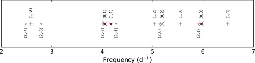
Comparison between the observed (red circles) and theoretical frequencies. Crosses, pluses, and triangular markers refer to l = 0, 1, and 2 modes, respectively. Each symbol is assigned to two numbers which correspond with the spherical degree l and radial order n.
Fig. 7 illustrates quality of the fit between the observed and theoretical frequencies based on our best-fitting evolutionary model. The observed values are shown by red dots, theoretical frequencies are presented by crosses (l = 0), pluses (l = 1), and triangular markers (l = 2). The dominant mode f1 = 4.0515 d−1 (46.8759 μHz) of the primary is identified as the fundamental radial mode, frequencies f3 = 4.1726 d−1 (48.2770 μHz) and f5 = 5.9706 d−1 (69.0201 μHz) are found to be the l = 1 non-radial mode and the second overtone radial mode, respectively, which is fully consistent with the spectroscopic mode identification of the two low-amplitude modes.
8 DISCUSSION AND CONCLUSIONS
In this paper, we presented a detailed spectroscopic study of the close pair of the σ Sco quadruple system. The analysis was based on some 1000 high-resolution, high-S/N spectra taken during three consecutive years, in 2006, 2007, and 2008.
We used two different approaches to determine the precise orbital elements of the close pair of two B-type stars. The first method relies on the iterative approach comprising of the determination of the orbital elements, the analysis of the residuals to extract the pulsation frequencies, and the cleaning of the original data from the pulsation signal. The cycle was repeated until we could get to a self-consistent set of orbital elements and pulsation frequencies of the primary. The second approach was based on the SPD technique, where the step of RV determination is overcome and orbital elements are optimized together with the disentangled spectra of both binary components. We found that this latter step suffers from the large-amplitude RV variations intrinsic to the primary component and it was impossible to obtain reliable disentangled spectra without a priori assumption on the RV semi-amplitude K1 of the primary. This assumption was made from the iterative approach outlined above; the obtained disentangled spectra were analysed to determine fundamental parameters and atmospheric chemical composition of both binary components.
The spectrum analysis was based on the non-LTE spectral synthesis and revealed two stars of the same effective temperature (spectral type) but different surface gravity (luminosity class). The primary was found to contribute about 62 per cent to the total light of the system; the individual components have a similar atmospheric chemical composition consistent with the present-day CAS (Nieva & Przybilla 2012). The spectroscopic flux ratio of ∼1.63 agrees within 1σ and 2σ error bars with the luminosity ratio from Tables 8 and 10, respectively. We found a low helium abundance for the secondary component which we do not trust to be real and attribute it to the problems we encountered during the disentangling of the spectrum of the secondary in the regions of strong He i lines. This is the first time that detailed abundance analysis is presented for both components of the σ Sco binary, and the first time that precise fundamental parameters are determined for the secondary component. The effective temperature of the secondary is in agreement with the value inferred by North et al. (2007) from the spectral type of the star. For the primary, our parameters are in agreement with most recent spectroscopic estimates (e.g. Niemczura & Daszyńska-Daszkiewicz 2005).
Fundamental parameters of both components of the σ Sco system, after seismic modelling.
| Parameter | Unit | Primary | Secondary |
|---|---|---|---|
| Mass (m) | M⊙ | 13.5|$^{+0.5}_{-1.4}$| | 8.7|$^{+0.6}_{-1.2}$| |
| Radius (R) | R⊙ | 8.95|$^{+0.43}_{-0.66}$| | 3.90|$^{+0.58}_{-0.36}$| |
| Luminosity (log(L)) | L⊙ | 4.38|$^{+0.07}_{-0.15}$| | 3.73|$^{+0.13}_{-0.15}$| |
| Age of the system | Myr | 12.1|$^{+2.0}_{-1.0}$| | |
Our spectroscopic data revealed three independent pulsation modes intrinsic to the primary component. The two dominant modes f1 = 4.0515 d−1 (46.8759 μHz) and f3 = 4.1726 d−1 (48.2770 μHz) were previously reported in several studies and identified as a radial (e.g. Cugier & Boratyn 1992; Heynderickx 1994) and l = 2 non-radial modes (Cugier & Boratyn 1992), respectively. The lowest amplitude mode f5 = 5.9706 d−1 (69.0201 μHz) detected in our spectroscopic data is in excellent agreement with the one found by Jerzykiewicz & Sterken (1984) in the differential uvby photometry. All other variability detected in the spectral lines of the primary component occurs either at harmonics of the dominant pulsation mode or at low-significance frequencies, which we do not consider as real ones.
By subtracting the contribution of the secondary from the composite spectra and by correcting the residuals for the orbital motion of the primary, we were able to perform spectroscopic mode identification for the two modes f3 and f5 (with f1 being postulated to be a radial mode) of the primary of σ Sco. The identification was done with two different methods, Fourier-parameter fit and moment method. The former technique seems to be inapplicable to our data, probably due to the insufficient rotational broadening of the spectral lines. The moment method delivers unambiguous identification for both modes, delivering (l, m) = (1,1) for f3 and a radial mode for f5. The inclination angle of the rotation axis of the primary with respect to the line of sight ranges from 17° to 32°. Combined with the orbital inclination reported by North et al. (2007), this suggests alignment or at most a small misalignment for the primary component of σ Sco. With the measurement of the inclination angle of the primary, we are able to constrain its equatorial rotation velocity to be between 60 and 110 km s−1, implying that the star rotates between 13.5 and 25 per cent of its break-up velocity.
We used our orbital elements together with the (interferometric) orbital inclination angle estimate from North et al. (2007) to compute individual masses and radii of both components of σ Sco. The values of the radii obtained this way agree within the estimated errors with those computed from angular diameters presented by North et al. (2007). In order to verify the mass and radius of the primary component, we performed the fitting of all three independent pulsation modes, using mesa and gyre – stellar evolution and oscillation codes, respectively. Our best-fitting theoretical model delivers an effective temperature and surface gravity in good agreement with the spectroscopic values, and confirms the radius of the primary determined from our orbital solution. The age of the system is estimated to be ∼12 Myr. Table 10 summarizes the final fundamental parameters of both components of σ Sco, where the mass and radius of the secondary were computed from the theoretical mass of the primary and spectroscopic mass ratio, and from the calculated mass and spectroscopic log g, respectively. The 1σ errors given in Tables 9 and 10 do not take into consideration systematic uncertainties connected with the choice of a given stellar evolution code and its input physics. Fig. 8 shows the position of both components of the σ Sco system in the Teff–log g diagram, along with the evolutionary tracks. The error bars are those obtained from the evolutionary models and 3σ spectroscopic uncertainties for the primary and secondary, respectively. The primary is an evolved star near the end of its main sequence, whereas the secondary just started its main-sequence evolution. The position of the secondary in the diagram suggests that the star is more massive than 8.7 M⊙, the mass we obtained from binary dynamics and the theoretical mass of the primary. Similar discrepancy was found for the main-sequence secondary component of the V380 Cyg binary system (Tkachenko et al. 2014).
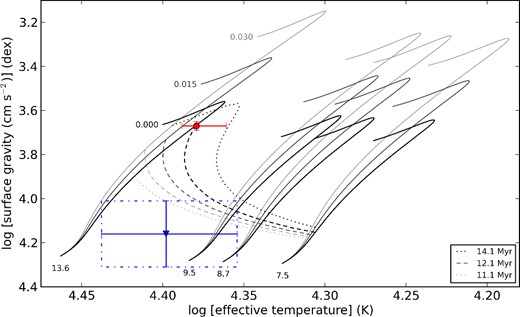
Position of the primary (circle) and the secondary (triangle) of σ Sco system in the Teff–log g diagram, along with the mesa evolutionary tracks. The initial masses as well as the overshoot parameter fov are indicated in the plot. The atmospheric parameters Teff and log g of the primary and secondary are those from asteroseismic and spectroscopic analysis, respectively. The isochrones corresponding to the age of the system of 12.1 Myr deduced from seismology of the primary are indicated by the dashed lines. The error range in age is given by the dotted lines, which correspond to the best-fitting overshoot parameter of the primary fov = 0.0.
Our asteroseismic analysis of the primary of σ Sco delivered the identification of all three fitted frequencies. This way, two of them, f1 and f5, are found to be fundamental and second overtone radial modes, respectively, and frequency f3 is identified as an l = 1 non-radial mode. This is in perfect agreement with the spectroscopic mode identification we obtained for f3 and f5 using the moment method. Identification for f1 is consistent with the majority of the previous studies (e.g. Cugier & Boratyn 1992; Heynderickx 1994) whereas the identification of f3 is different from the one previously found by Cugier & Boratyn (1992). The mode identification for f5 presented in this study is done for the first time. The addition of the seismic constraints to the modelling implied a drastic reduction in the uncertainties of the fundamental parameters, and provided an age estimate. Our best-fitting evolutionary model suggests a small decrease of 7.3 × 10⁻⁵ d−1 century−1 of the frequency of the dominant radial mode; the effect cannot be detected from our data due to low-frequency resolution.
This paper is the second one in a series devoted to the analysis of spectroscopic double-lined binary systems, consisting of two B-type stars of which at least one is a pulsating star. We find a fully consistent solution and agreement with stellar models for the primary component, after having taken into account its pulsational behaviour in the analysis of the data. These conclusions are in sharp contrast with the incompatibility between data and models for the binary V380 Cyg, for which we found a discrepancy of ∼1.5 M⊙ between the dynamical and theoretical mass and a huge core overshoot was needed to explain the properties of the primary. On the other hand, the fact that V380 Cyg is an eclipsing double-lined spectroscopic binary allowed us to measure the masses of individual component to precisions approaching 1 per cent, while precisions in masses of both components of the σ Sco system are as bad as ∼30 per cent if we do not consider the seismic properties of the primary. In this respect, the two systems are incomparable and purely measured dynamical masses of the σ Sco stellar components prevent us from drawing any firm conclusions with respect to the theoretical models. In our next paper, we will present a detailed analysis of the Spica system, based on the space-based photometric and ground-based high-resolution spectroscopic data.
The research leading to these results has received funding from the European Community's Seventh Framework Programme FP7-SPACE-2011-1, project number 312844 (SPACEINN), and from the Fund for Scientific Research of Flanders (FWO), Belgium, under grant agreement G.0B69.13. Mode identification results with the software package famias developed in the framework of the FP6 European Coordination Action HELAS (http://www.helas-eu.org/).
E-mail: [email protected]
