


Abstract
We assess the effects of supermassive black hole (SMBH) environments on the gravitational wave (GW) signal from binary SMBHs. To date, searches with pulsar timing arrays for GWs from binary SMBHs, in the frequency band ∼1–100 nHz, include the assumptions that all binaries are circular and evolve only through GW emission. However, dynamical studies have shown that the only way that binary SMBH orbits can decay to separations where GW emission dominates the evolution is through interactions with their environments. We augment an existing galaxy and SMBH formation and evolution model with calculations of binary SMBH evolution in stellar environments, accounting for non-zero binary eccentricities. We find that coupling between binaries and their environments causes the expected GW spectral energy distribution to be reduced with respect to the standard assumption of circular, GW-driven binaries, for frequencies up to ∼20 nHz. Larger eccentricities at binary formation further reduce the signal in this regime. We also find that GW bursts from individual eccentric binary SMBHs are unlikely to be detectable with current pulsar timing arrays. The uncertainties in these predictions are large, owing to observational uncertainty in SMBH–galaxy scaling relations and the galaxy stellar mass function, uncertainty in the nature of binary–environment coupling and uncertainty in the numbers of the most massive binary SMBHs. We conclude, however, that low-frequency GWs from binary SMBHs may be more difficult to detect with pulsar timing arrays than currently thought.
1 INTRODUCTION
The merger of a pair of galaxies hosting central supermassive black holes (SMBHs) is expected to result in the formation of a binary SMBH (Begelman, Blandford & Rees 1980). The central SMBHs sink in the merger remnant potential well through the action of dynamical friction, and form a bound binary when the mass within the orbit of the lighter SMBH is dominated by the heavier SMBH. As stars within the binary orbit are quickly ejected, the binary will decay further only if another mechanism to extract binding energy and angular momentum exists. Proposed mechanisms include slingshot scattering of stars on radial, low angular momentum orbits intersecting the binary (Frank & Rees 1976; Quinlan 1996; Yu 2002), and friction against a spherical Bondi gas accretion flow (Escala et al. 2004) or a circumnuclear gas disc (e.g. Roedig et al. 2011). If the orbital decay process can drive the binary to a small separation, gravitational wave (GW) emission will eventually cause the binary to coalesce (e.g. Peters & Mathews 1963; Baker et al. 2006).
In a cosmological context, merging dark matter haloes follow parabolic trajectories (e.g. van den Bosch et al. 1999; Wetzel 2011), implying large initial eccentricities (typically ∼0.6; Hashimoto, Funato & Makino 2003) for the orbits of SMBHs sinking towards galaxy merger remnant centres. Steep stellar density gradients in merging galaxies may reduce this eccentricity; indeed, some models suggest that binary SMBHs are likely to be close to circular upon formation (Casertano, Phinney & Villumsen 1987; Polnarev & Rees 1994; Hashimoto, Funato & Makino 2003). Slingshot interactions between binaries and individual stars again grow the eccentricities (e.g. Quinlan 1996; Sesana, Haardt & Madau 2006; Berentzen et al. 2009; Khan et al. 2012), because binaries spend more time, and hence lose more energy, at larger separations. Roedig et al. (2011) found that binary SMBHs embedded in massive self-gravitating gas discs will have large eccentricities, between 0.6 and 0.8, at the onset of GW-dominated evolution. In the GW-dominated regime, however, binaries are expected to quickly circularize (e.g. Peters & Mathews 1963; Baker et al. 2006).
There is no direct observational evidence for the existence of binary SMBHs (Dotti, Sesana & Decarli 2012). However, the GW emission from binaries prior to coalescence is an unambiguous signature of their existence. Observing GWs from binary SMBHs will enable binary SMBH physics, as well as models for the formation and evolution of the cosmological SMBH population, to be observationally tested. Here, we focus on the possibility of detecting GWs from binary SMBHs in the early parts of their GW-dominated evolutionary stages with radio pulsar timing arrays (PTAs; Foster & Backer 1990; Manchester et al. 2013). PTAs are currently sensitive to GWs in the frequency band ∼1–100 nHz, which is complementary to other GW detection experiments.
PTAs target both a stochastic, isotropic background of GWs from binary SMBHs (e.g. van Haasteren et al. 2011; Yardley et al. 2011) and GWs from individual binary systems (Yardley et al. 2010; Ellis, Siemens & Creighton 2012). The summed GW signal from all binary SMBHs in the Universe is expected to approximate an isotropic background, although individual binaries are potentially detectable at all frequencies within the PTA band (Ravi et al. 2012). Recent PTA results suggest that a large fraction of existing models for the GW background from binary SMBHs are inconsistent with observations (Shannon et al. 2013). However, most current predictions for the spectral shape (Phinney 2001), statistical nature (Sesana, Vecchio & Volonteri 2009; Ravi et al. 2012) and strength (Sesana 2013a) of the GW signal from binary SMBHs assume that all binaries are in circular orbits, and losing energy and angular momentum only to GWs. These assumptions correspond to the well-known power-law GW background characteristic strain spectrum from binary SMBHs that is proportional to f−2/3, where f is the GW frequency.
Here, we present an examination of the properties of the GW signal from binary SMBHs given a realistic model for binary orbital evolution. We use a semi-analytic model for galaxy and SMBH formation and evolution (Guo et al. 2011, hereafter G11) implemented in the Millennium simulation (Springel et al. 2005) to specify the coalescence rate of binary SMBHs, and augment this with a framework (Sesana 2010) for the evolution of binary SMBHs in stellar environments. We neglect gas-driven binary evolution. This is because massive galaxies at low redshifts, which are expected to dominate the GW signal from binary SMBHs, will typically be late type and gas poor (e.g. Yu et al. 2011).
Two key phenomena in binary SMBH evolution affect the summed GW signal relative to the case of circular binaries evolving under GW emission alone.1
Interactions between binary SMBHs and their environments will accelerate orbital decay compared to purely GW-driven binaries, reducing the time each binary spends radiating GWs. This may reduce the energy density in GWs at the lower end of the PTA frequency band (e.g. Wyithe & Loeb 2003; Sesana 2013b).
While circular binaries emit GWs at the second harmonics of their orbital frequencies, eccentric binaries emit GWs at multiple harmonics (Peters & Mathews 1963). Given a population of binary SMBHs this is expected to transfer GW energy density from lower frequencies in the PTA frequency band to higher frequencies (Enoki & Nagashima 2007; Sesana 2013b).
We consider the effects of both these phenomena on the GW signal from binary SMBHs relative to the circular, GW-driven case. We also examine the possibility of detecting bursts of GWs from individual eccentric, massive binaries. In Section 2, we outline the binary population model. We give our predictions for the summed GW signal in Section 3, along with a discussion of uncertainties in our model. We consider the possibility of detectable GW bursts in Section 4. Finally, we summarize our results in Section 5 and present our conclusions in Section 6. Summaries of key PTA implications can be found at the ends of Sections 3, 4 and 5. We adopt a concordance cosmology consistent with the Millennium simulation (Springel et al. 2005), with ΩM = 0.25, Ωb = 0.045, ΩΛ = 0.75 and H0 = 73 km s−1 Mpc−1.
2 DESCRIPTION OF MODELLING METHODS
2.1 The gravitational wave background from a cosmological source population
2.2 The binary SMBH population at formation
We adopt a simple, one-parameter distribution for the eccentricities of binary SMBHs at formation, based on the postulate that the semimajor and semiminor axes of the orbits (a0 and b0, respectively) are each log-normally distributed. This is justified because (a) while many stellar encounters influence the values of a0 and b0, the effects of these encounters on the parameter values are heterogeneous, and (b) both a0 and b0 are strictly positive.2 In general, log-normal distributions are used to model positive-definite random variables that are influenced by many multiplicative effects of differing magnitudes (i.e. heterogeneous effects). The central limit theorem implies that the product of a large number of finite-variance positive random variables will approximately have a log-normal distribution.
We use the publicly available results (Lemson & Virgo Consortium 2006) of the semi-analytic model of G11 to specify |$D_{\boldsymbol {\zeta }_{0}}[N(\boldsymbol {\zeta }_{0},z)]$|. As outlined in Ravi et al. (2012) and Shannon et al. (2013), the G11 results can be used to predict the coalescence rate of binary SMBHs. For this work, we only use coalescences with both M1 and M2 greater than 106 M⊙, and only draw from the implementation of the G11 model in the Millennium simulation. We scale all SMBH masses by a factor of 1.9 (Shannon et al. 2013) to account for recent SMBH and galaxy bulge measurements.
We relate the dark matter halo virial velocities, Vvir, of galaxies in the G11 model to spheroid stellar velocity dispersions σ (Baes et al. 2003; Marulli et al. 2008). This assumption is discussed further in Section 3.3.2. For each bin of z, M1 and M2, we find the average velocity dispersions of recently merged galaxies in the G11 model hosting an SMBH of mass M1 + M2. We use these values to specify aH for each bin of the discrete distribution |$n(\boldsymbol {\zeta }_{0},z)$|.
2.3 Evolution of binary SMBH orbits to the GW regime
We assume that all SMBH binary orbits decay through interactions with fixed, isotropic, unbound cuspy stellar backgrounds, and through GW emission. The former scenario has been extensively studied numerically by Quinlan (1996), Sesana et al. (2006) and Sesana (2010). We assume a power-law stellar density distribution within the binary gravitational influence radius for all galaxies prior to mergers. For the majority of this paper, we additionally assume a stellar density profile power-law index of γ = 1.5 corresponding to a mild stellar cusp (see equation 1 of Sesana 2010). We consider variations in these assumptions further in Section 3.3.2.
We evolve the binary eccentricities, e, and semimajor axes, a, through scattering by unbound stars and loss of energy and angular momentum to GWs using expressions for |$\frac{{\rm d}a}{\rm{d}t_{{\rm r}}}$| and |$\frac{\rm{d}e}{\rm{d}t_{{\rm r}}}$| from equations (15) and (16) of Sesana (2010). The effects of the ejection of stars that are bound to the SMBHs (Sesana, Haardt & Madau 2008a) are significant only for binary separations greater than ah, and we hence neglect this phenomenon.
We use the fits of Sesana et al. (2006) for the rates of evolution of binary semimajor axes and eccentricities based on numerical scattering experiments (the ‘H’ and ‘K’ coefficients, respectively, from tables 1 and 3 of Sesana et al. 2006). We log-interpolate the published values at binary component mass ratios of interest. As Sesana et al. (2006) only provide rates of semimajor axis evolution for circular binaries, we assume here that the rate of semimajor axis evolution at a given semimajor axis is independent of eccentricity. This approximation leads to the semimajor axis evolution rate being underestimated by at most 20 per cent for the most eccentric binaries (see fig. 3 of Sesana et al. 2006). We also only use the seven values for our initial binary eccentricities (i.e. e0) considered by Sesana et al. (2006); see their table 3. These are 0, 0.15, 0.3, 0.45, 0.6, 0.75 and 0.9.
To then specify the population of GW-emitting binary SMBHs, we need to calculate the numbers of binaries with different orbital frequencies. The GW luminosity, L, per unit frequency, fr, of a binary SMBH depends on the masses M1 and M2, the eccentricity e and the orbital frequency forb (Peters & Mathews 1963). The functional form of |$L(f_{{\rm r}},\boldsymbol {\zeta })$| is given in, for example, equation (2.6) of Enoki & Nagashima (2007). We now define a new parameter vector |$\boldsymbol {\zeta }=[M_{1},M_{2},e,f_{{\rm orb}}]$|.
3 PREDICTIONS FOR THE CHARACTERISTIC STRAIN SPECTRUM
3.1 Results
As stated above, we consider four different initial eccentricity distributions: w0 = 0, 0.1, 0.35, 0.93. Recall that the w0 = 0 case corresponds to all binaries being circular. Initially circular binaries are not expected to become eccentric (e.g. Sesana 2010). The probability mass functions of the binary eccentricities, e0, at aH in the three cases with w0 > 0 are shown in Fig. 1. For comparison, we also show in the bottom panel of Fig. 1 a ‘thermal’ probability mass function for e0, derived from the probability density function |$f_{e_{0}}=2e_{0}$| for 0 ≤ e0 ≤ 1. This would be expected if binary systems followed a purely Maxwell–Boltzmann distribution of energies (e.g. Ambartsumian 1937), as is roughly the case for galactic stellar binaries (Duquennoy & Mayor 1991).
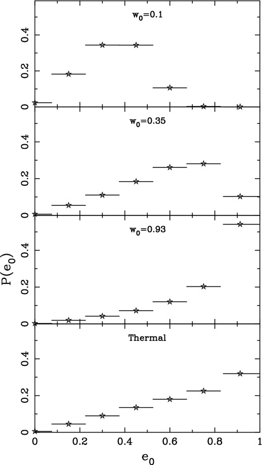
Probabilities, P(e0), of obtaining different values of e0 (indicated by stars) for three initial eccentricity distributions defined by w0 = 0.1, 0.35, 0.93 and equation (7) (top three panels), and for a thermal eccentricity distribution (bottom panel). The values of e0 correspond to those considered by Sesana et al. (2006); see text for details.
In Fig. 2, we plot the characteristic strain spectra for each initial eccentricity distribution. Also depicted is the prediction in the circular (i.e. w0 = 0), GW-driven case (i.e. for |$\frac{\rm{d}a}{\rm{d}t_{\rm r}}$| including only GW-driven orbital decay for all a). This latter prediction corresponds to the standard hc(f)∝f− 2/3 power law. In order to help highlight the physical effects at work, Fig. 3 shows the characteristic strain spectra for each assumed w0 contributed by binaries with combined masses in the ranges 106.5–1010 and 1010–1011 M⊙, respectively.
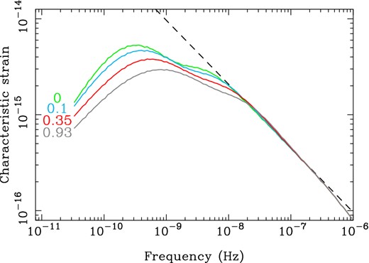
The solid lines depict characteristic strain spectra for w0 = 0 (green), w0 = 0.1 (blue), w0 = 0.35 (red) and w0 = 0.93 (grey); the w0 values for each line are given at the left of the plot. All curves were calculated assuming a stellar density profile index of γ = 1.5. The black dashed line is the characteristic strain spectrum assuming circular orbits and purely GW-driven evolution for all SMBH binaries.

Characteristic strain spectra contributed by binaries with total masses in the range 106.5–1010 M⊙ (dashed curves) and in the range 1010–1011 M⊙ (solid curves). The colours represent different values of w0 as in Fig. 2; note that the orders of the low- and high-mass curves from top to bottom correspond to increasing w0 as in Fig. 2. We again show the characteristic strain spectrum for all SMBH binaries assuming circular orbits and purely GW-driven evolution as a black dashed line.
The model we utilize for interactions between binaries and their stellar environments results in an attenuation of hc(f) in the PTA frequency band compared to the f−2/3 power law obtained in the circular, GW-driven case. For w0 = 0, the signal is attenuated at frequencies f ≲ 10−8 Hz. At these frequencies, stellar interactions are the dominant binary orbital decay process, increasing |$\frac{\rm{d}f_{{\rm orb}}}{\rm{d}t_{\rm r}}$| in equation (12) and reducing the number of binaries observed per unit orbital frequency. For increasing w0, the signal is further attenuated at low frequencies, although a slight (∼0.01 dex), increasing excess is present at frequencies between 10−8 and 10−7 Hz. This is caused by two effects: eccentric binaries evolve faster than circular binaries, and eccentric binaries radiate GWs at higher harmonics of their orbital frequencies than circular binaries.
The ‘substructure’, or two bumps, in the characteristic strain spectra is a direct consequence of the mass distribution of the binaries in our model. If |$D_{\boldsymbol {\zeta }_{0}}[N(\boldsymbol {\zeta }_{0},z)]$| were smooth and analytic, the characteristic strain spectra would have only one clear peak. Here, however, we evaluate this distribution from the G11 semi-analytic model outputs (see equation 8), which results in the distribution being incomplete at the high-mass end. These gaps in the distribution lead to the two apparent peaks in the characteristic strain spectra.
As is evident in Fig. 3, the first peaks of the spectra in Fig. 2 are dominated by the highest mass binaries, whereas the second peaks are dominated by lower mass binaries. This is because the evolution of the highest mass binaries begins to be GW driven at lower frequencies than for less massive binaries. There are expected to be very few binaries in the (combined) mass range 1010–1011 M⊙; only ∼50 with forb ≥ 10−12 Hz are expected to be present in the observable Universe according to the G11 model. In contrast, ∼5 × 10⁶ binaries are expected the range 106.5–1010 M⊙. The effects of sparsity in |$D_{\boldsymbol {\zeta }_{0}}[N(\boldsymbol {\zeta }_{0},z)]$| are discussed further in Section 3.3.3.
3.2 Comparison with previous work
Our results for the GW characteristic strain spectra from an eccentric binary SMBH population are broadly consistent with similar previous studies (Enoki & Nagashima 2007; Sesana 2013b). Both these works find spectra which depart from the standard power law of the circular, GW-driven case at frequencies f < 10−8 Hz. The results of Sesana (2013b) for binaries with eccentricities at formation of 0.7 are in fact very similar to ours (see their fig. 2), with slight substructure evident along with the slight excess for f > 10−8 Hz.
Our results for w0 = 0, however, differ somewhat from those of Sesana (2013b). Whereas the maximum separation between the zero-eccentricity and high-eccentricity curves (the red solid and dashed curves in fig. 2 of Sesana 2013a) is approximately 0.5 dex, the maximum difference between our curves for w0 = 0 and 0.93 in our Fig. 2 is 0.35 dex. We also find similarly shaped spectra for all w0, whereas Sesana (2013b) has a clear single peak in their zero-eccentricity curve.
The differences between our results and those of Sesana (2013b) for w0 = 0 are caused by the nature of the respective binary SMBH mass distributions used. As discussed above, if the mass distribution of binary SMBHs (|$D_{\boldsymbol {\zeta }_{0}}[N(\boldsymbol {\zeta }_{0},z)]$|) were smooth and analytic, which is the case in Sesana (2013b), only a single peak is expected. The reason for the similarity between our results and those of Sesana (2013b) for non-zero eccentricities may be because of some discreteness in the eccentric binary SMBH distribution used by Sesana (2013b), as evidenced by the jagged nature of their strain spectrum at low frequencies.
The characteristic strain spectrum we predict in the circular, GW-driven case is ∼0.15 dex lower than that predicted by Shannon et al. (2013). This difference is because we do not fit an analytic function to the discrete binary distribution |$n(\boldsymbol {\zeta }_{0},z)$|. We discuss this point further in Section 3.3.3.
3.3 Uncertainties in the model predictions
In this section, we describe the key uncertainties in our prediction of hc(f), which are summarized in Fig. 4. We consider in turn the accuracy of the model predictions for SMBH demographics and coalescence rates and for the rate of evolution of binary systems, and the effects of incomplete high-mass binary SMBH distributions.
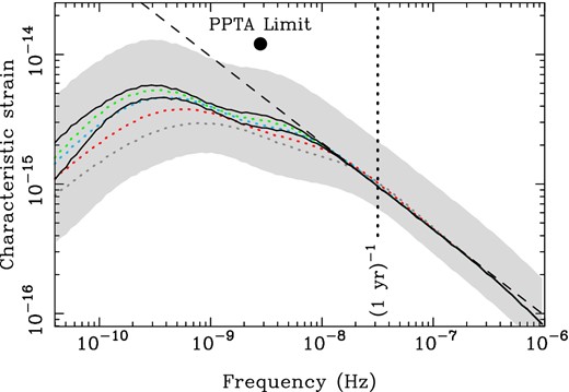
The four coloured dotted curves are the characteristic strain spectra for the four w0 cases we consider, also shown with the same colours in Fig. 2. The upper solid black curve corresponds to a stellar density profile index of γ = 1, and the lower solid black curve corresponds to γ = 2; both are calculated assuming w0 = 0, and so may be compared with the green (uppermost, w0 = 0) dotted curve. The grey shaded area represents an approximate 68 per cent confidence interval in our prediction of hc(f), given observational errors in the SMBH–bulge mass relation and the galaxy stellar mass function (a 0.4 dex range), allowing for the full range of w0 values, and including a possible increase of 0.15 dex in the predictions if the binary SMBH population statistics were accurately specified (Shannon et al. 2013). The black dot indicates the most recent 95 per cent confidence upper limit on the stochastic Gaussian GW signal (Shannon et al. 2013, see text for details). The characteristic strain spectrum calculated here in the circular, GW-driven case (and shown in Figs 2 and 3) is displayed as a black dashed line. The vertical dotted line indicates a frequency of (1 yr)−1.
3.3.1 SMBH demographics and coalescence rates
The merger rate of massive galaxies predicted by galaxy formation models (Bertone, De Lucia & Thomas 2007) implemented in the Millennium simulation (Springel et al. 2005) has been shown to be consistent with observational estimates at redshifts z < 2 (Bertone & Conselice 2009). Marulli et al. (2008) found that the model matches the observed quasar bolometric luminosity function at redshifts z ≤ 1 for a variety of assumed quasar light curves. This, together with the reproduction of the local SMBH–galaxy scaling relations, suggests that the rate of formation of massive binary SMBHs at low redshifts is satisfactorily reproduced by the G11 semi-analytic model, which is used as the basis for this paper. Furthermore, the characteristic strain spectrum expected in the w0 = 0 case for binaries with combined masses M1 + M2 > 2 × 10⁸ M⊙ at redshifts z ≤ 1 has a maximum disparity with the unrestricted spectrum of 0.02 dex. Hence, our model robustly predicts the contribution to the GW signal from massive, low-redshift binaries, which are likely to dominate the total GW signal (see also Wyithe & Loeb 2003; Sesana 2013a).
However, there remain a range of theoretical uncertainties. For example, the G11 model treatment of SMBHs does not include physically motivated prescriptions for SMBH formation (e.g. Haiman 2013), SMBH ejection caused by gravitational recoil following the coalescence of binary systems (e.g. Kulier et al. 2013) and does not account for any mass accreted on to SMBHs in merging galaxies prior to coalescence (e.g. Van Wassenhove et al. 2012).
There are also specific observational uncertainties in tuning the semi-analytic model. The current sample of SMBH and host galaxy bulge mass measurements, which is used to tune the quasar-mode SMBH accretion efficiency, allows for a 1σ confidence interval of ∼0.2 dex in the SMBH masses (Shannon et al. 2013). Similarly, the galaxy stellar mass function predicted by the G11 model is matched to Sloan Digital Sky Survey observations in the nearby Universe (e.g. Li & White 2009). These observations have a ∼0.2 dex systematic uncertainty, with negligible contribution from cosmic variance (Li & White 2009), which corresponds (to first order) to a ∼0.3 dex uncertainty in the galaxy merger rate.
The uncertainty in SMBH masses corresponds to a ∼0.3 dex uncertainty in ΩGW(f), while the uncertainty in the merger rate translates directly to the range of predictions for ΩGW(f) allowed by the observed galaxy stellar mass function. Combining both ranges results in a 0.4 dex (1σ) uncertainty in ΩGW(f), which corresponds to a 0.2 dex uncertainty in hc(f).
3.3.2 The binary evolution model
In this paper, we assume that all galaxies hosting SMBHs have spherically symmetric central stellar density profiles that are power-law functions of radius, r, following Sesana (2010). That is, the stellar density, ρ(r), is proportional to r−γ, where we have hitherto assumed γ = 1.5. These profiles are equivalent to the central (asymptotic) behaviour of the Dehnen (1993) stellar potential and density models, which correspond well to high-resolution observations of the centres of nearby galaxy bulges (Faber et al. 1997). Our assumption of a universal γ is, however, not in agreement with observations, which typically show 1 ≲ γ ≲ 2, with γ = 1 corresponding to the most extreme ‘core’ galaxies and γ = 2 corresponding to the most extreme ‘power-law’ galaxies (Dehnen 1993; Faber et al. 1997). Furthermore, ‘core’ galaxies are generally more massive, early-type systems with more massive SMBHs, and ‘power-law’ galaxies are generally less massive, late-type systems with less massive SMBHs (e.g. Faber et al. 1997; McConnell & Ma 2013). While we do not attempt to correlate γ with galaxy properties from the G11 model, we show in Fig. 4 characteristic strain spectra in the w0 = 0 case for γ = 1 and 2. The logarithmic differences between the spectra for these γ values and the w0 = 0 spectrum for γ = 1.5 may be applied only approximately to the spectra for other w0 values, because varying γ varies both the rate of semimajor axis decay and the rate of eccentricity evolution for binaries.
The model that we use (Sesana et al. 2006; Sesana 2010) for binaries evolving through separations less than aH due to interactions with fixed stellar backgrounds is qualitatively similar to the results of recent numerical simulations of dry (i.e. free of dynamically significant gas) galaxy merger remnants (Khan et al. 2012). However, as we show in Appendix A, it is apparent that the model we use includes stronger stellar-driven orbital decay than the simulations of Khan et al. (2012). This is despite our assumption (see Section 2.2) that the rate of semimajor axis evolution is independent of binary eccentricity. This is not surprising, because the assumption of a fixed stellar background is qualitatively equivalent to the assumption of a full stellar loss cone (cf. Quinlan & Hernquist 1997; Sesana 2010). Hence, the model we use maximizes binary orbital decay rates, in particular for spherically symmetric stellar distributions.
We are likely therefore to be overestimating the effects of stellar interactions on the binary SMBH population. The numerical simulations of Khan et al. (2012) suggest that the orbital frequencies at which binary SMBH evolution begins to be predominantly GW driven are up to 0.45 dex less than the corresponding frequencies that result from the model we use. This implies that the frequency below which the characteristic strain spectrum turns over from the hc(f)∝f− 2/3 power law may be up to 0.45 dex lower than we predict.
While the Vvir–σ relation that we assume is established in the local Universe (Baes et al. 2003), it has not been studied at higher redshifts. Given the expected decrease in the stellar mass in a halo of a given mass with increasing redshift (Moster et al. 2010), it is possible that we are overestimating the velocity dispersions of the stellar cores of merger remnants beyond the local Universe. This would imply that higher redshift binaries decay more slowly than in our model, again increasing the low-frequency parts of the presented characteristic strain spectra. Further work is required to quantify the magnitude of this increase.
Finally, while the assumed functional form of the e0 distribution (equation 7) is physically motivated, there may be some correlation between the orbital eccentricities of binaries with separations aH, and their masses and redshifts. Additionally, a variety of studies find physical reasons for binaries to be quite circular upon formation (Casertano et al. 1987; Polnarev & Rees 1994; Hashimoto et al. 2003), which suggests that low-w0 values may be preferred. Current numerical simulations (e.g. Khan et al. 2012) have not been run with a sufficient range of initial conditions to provide conclusive results on this point.
3.3.3 Accounting for discreteness in the binary SMBH distributions from the G11 model
Given the distribution |$n(\boldsymbol {\zeta }_{0},z)$| (equation 8, Section 2.2) of binary SMBHs, we have examined the expected value of the GW characteristic strain spectrum. However, the binary SMBH distribution that we use is not exactly the distribution expected from the G11 semi-analytic model implemented within the Millennium simulation. The Millennium simulation provides a single realization of the dark matter halo merger history within a large comoving volume, and the G11 prescriptions specify properties of the galaxies, and SMBHs, associated with the haloes. To form the discrete binary distribution |$n(\boldsymbol {\zeta }_{0},z)$|, we count the numbers of binary SMBHs forming in the entire Millennium volume between redshift snapshots in bins of M1 and M2, assigning values of e0 to each binary according to our e0 distribution. However, despite the large volume, |$n(\boldsymbol {\zeta }_{0},z)$| is poorly populated for high M1 and M2 at every redshift. To estimate the expected nature of this distribution, statistical modelling is required. This was done by Shannon et al. (2013), who considered the circular, GW-driven case, and found that the modelling resulted in a characteristic strain spectrum increased by 0.15 dex. However, the distribution |$n(\boldsymbol {\zeta }_{0},z)$| has two more dimensions (an extra mass dimension and the eccentricity dimension) than that considered by Shannon et al. (2013), which significantly complicates the modelling. Instead, we simply consider it possible that the strain spectrum we have derived may be up to 0.15 dex larger.
A qualitatively similar effect was pointed out by Sesana, Vecchio & Colacino (2008b), who compared characteristic strain spectra generated from realizations of the binary SMBH population of the universe to the spectrum expected on average, in the circular, GW-driven case. Whereas the average spectrum was a power law proportional to f−2/3, individual realizations had a lower amplitude at higher frequencies. This was because the numbers of binaries radiating GWs at a given frequency (per unit frequency) decreases with increasing frequency, implying that, for example, there is a frequency above which the expected number of sources is less than unity. However, the correct model for the average characteristic strain spectrum still had hc(f)∝f− 2/3 for all f, despite all realizations of the spectrum being below this power law at high frequencies. This situation is analogous to our suggestion of an increase in the characteristic strain spectrum if the average behaviour of |$n(\boldsymbol {\zeta }_{0},z)$| were correctly modelled.
We also do not attempt here to describe the statistical nature of the GW signal, as was done by Ravi et al. (2012) in the circular, GW-driven case. Ravi et al. (2012) modelled a GW signal that was mildly non-Gaussian, with individual sources dominant at all GW frequencies of interest to PTAs. Shannon et al. (2013) further showed that assuming non-Gaussian statistics for the GW signal caused constraints on ΩGW to degrade by ∼20 per cent. This reflects the fact that realizations of ΩGW(f) at a particular frequency f would have a larger variance in the non-Gaussian case than in the Gaussian case.
As discussed in Section 3.1, environment-driven binary evolution causes the highest mass binaries to dominate ΩGW(f) at low frequencies to a greater extent than in the purely GW-driven case. This, coupled with the sparsity of these binaries in our calculations, causes the low-frequency substructure in the characteristic strain spectra for all w0 in Fig. 2. Our results, however, suggest a more general conclusion: that, at low frequencies, environment-driven binary evolution causes the variance in realizations of ΩGW(f) to be significantly increased relative to the assumption of only GW-driven evolution. Including this increased variance in ΩGW(f) at low frequencies in the calculation of PTA upper bounds on ΩGW(f) (e.g. Shannon et al. 2013) would cause these constraints to be further degraded relative to constraints based on the work of Ravi et al. (2012).
3.3.4 Synthesis of uncertainties in hc(f)
We refer the reader to Fig. 4, where we show an approximate 1σ confidence interval on the characteristic strain spectrum according to the model we describe. This interval represents our uncertainty in the expected value of the signal, not the realization-to-realization uncertainty. The interval encompasses the maximum possible ranges of w0 and γ (see Section 3.3.2), and also includes observational uncertainties in the SMBH–bulge mass relation and in the galaxy stellar mass function (see Section 3.3.1). We also include our assertion that the characteristic strain spectrum could be up to 0.15 dex larger than what we calculate if the binary SMBH distribution were correctly specified (see Section 3.3.3).
It is clear that that there is relatively more uncertainty in our prediction at frequencies f ≲ 2 × 10⁻⁸ Hz, where environmental interactions and binary eccentricities may affect the signal. We have also not included our uncertainty in the specific model for environment-driven binary SMBH evolution. As discussed in Section 3.3.2, the model we use may represent the maximum level of binary–environment coupling; other models may result in the characteristic strain spectrum being boosted at low frequencies relative to our prediction. For example, the model of Khan et al. (2012) suggests that the effects of environmental interactions may only be relevant for f ≲ 7 × 10⁻⁹ Hz (also see Appendix A). We have also weighted each w0 value equally, whereas it is possible that low-w0 values are preferred over high-w0 values.
In Fig. 4, we also indicate the best upper bound on a stochastic, Gaussian GW background from binary SMBHs, published recently by the Parkes Pulsar Timing Array (PPTA; Shannon et al. 2013). This upper bound corresponds to ΩGW(2.8 nHz) < 1.3 × 10⁻⁹ with 95 per cent confidence. While PTA bounds are traditionally shown as wedges (e.g. Sesana et al. 2008b, fig. 13) on characteristic strain spectrum plots, Shannon et al. (2013) argued that their limit was applicable only at a single GW frequency. We hence display this limit as a single dot.
Our prediction for the characteristic strain spectrum at a frequency of f = (1 yr)−1 of 6.5 × 10− 16 < hc < 2.1 × 10− 15 (with approximately 68 per cent confidence) is broadly consistent with previous results (e.g. Wyithe & Loeb 2003; Sesana et al. 2008b; Sesana 2013a; Shannon et al. 2013) that considered the circular, GW-driven case. Indeed, for f ≳ 2 × 10⁻⁸ Hz, the predicted characteristic strain spectrum closely resembles the hc(f)∝f− 2/3 power law expected in the circular, GW-driven case, with the exception that for larger w0 slightly more signal is present. The departure from the f−2/3 power law at f ∼ 3 × 10⁻⁷ Hz is caused by binary SMBHs radiating at these frequencies reaching their last stable orbits and not being included in our calculations (see e.g. Wyithe & Loeb 2003).
3.4 Summary of PTA implications
Our results suggest a challenging future for attempts at detecting the GW background from binary SMBHs with PTAs. The frequency of optimal sensitivity for PTAs generally corresponds to the inverse of the characteristic observation time (e.g. Shannon et al. 2013). Typical observation times of 5–30 yr (Manchester et al. 2013) imply that the properties of the GW signal at frequencies in the range 5 × 10⁻¹⁰–10−8 Hz are of primary importance for PTA work. The model we use in this paper implies that the GW characteristic strain spectrum may be reduced throughout this frequency range relative to the circular, GW-driven case (i.e. with respect to a hc(f)∝f− 2/3 power law). For example, Shannon et al. (2013) presented a single-frequency constraint on ΩGW(f) that is inconsistent with a variety of astrophysical predictions assuming circular, GW-driven binaries. However, the constraint is at a frequency where the characteristic strain spectrum we predict (see Fig. 4) is reduced by at least 0.08 dex relative to the circular, GW-driven case. More generally, the gains in sensitivity to a GW background with observing time, estimated assuming hc(f)∝f− 2/3 (e.g. Siemens et al. 2013), are likely to be overestimated. Furthermore, it is possible that at low frequencies the increased contribution to the total GW signal of rare, massive binary SMBHs relative to the circular, GW case will cause the signal at these frequencies to be more non-Gaussian than suggested by Ravi et al. (2012).
However, our results require significant refinement. It is clear from Fig. 4 that our prediction for the characteristic strain spectrum at low frequencies is quite uncertain. Besides this uncertainty, the model we use in this paper for the coupling between binary SMBHs and stellar environments (Sesana et al. 2006; Sesana 2010) may in fact maximize the strength of this coupling (see Section 3.3.2 and Appendix A). Also, it is possible that lower eccentricity scenarios may be preferred over the higher eccentricity scenarios. Both the above possibilities would result in the low-frequency parts of the characteristic strain spectrum being increased relative to our predictions. We strongly urge further work on modelling the evolution of binary SMBH orbits in a variety of realistic galaxy merger scenarios. This is of significant importance for predicting the strength of the GW signal from binary SMBHs in the PTA frequency band.
4 PREDICTIONS FOR GW BURSTS
4.1 The distribution of GW bursts
The prospect of detecting GW bursts with PTAs has been pursued recently by a number of authors (e.g. Finn & Lommen 2010; Pitkin 2012). GW burst detection algorithms generally contain few assumptions about the source properties, except that they search for a strong signal confined to a short time period. Here, we focus on the properties of GW bursts from eccentric binary SMBHs, and use our distribution of binary SMBHs, |$D_{\boldsymbol {\zeta }}[N(\boldsymbol {\zeta },z)]$|, to predict the distribution of burst events.
It is necessary to form a definition of a GW burst from an eccentric binary SMBH in terms pulsar timing data products. Pulsar timing is the practice of measuring the times of arrival (ToAs) of pulses from millisecond radio pulsars and fitting a physical model to these measurements. In Appendix B, we describe how GWs from eccentric binaries affect pulsar timing measurements by inducing variations to ToAs. We present an expression for the rms deviation, σR(t), of the ToA variations as a function of time caused by a given binary SMBH in equation (B11), averaged over all orientation parameters.
In Fig. 5 , we show the orbital phase, θ, the expected energy flux in GWs at the Earth and σR(t) as functions of time for a binary SMBH with eccentricity 0.8 and orbital period at the Earth of 3.1 yr at the starting time, component masses M1 = 1010 M⊙ and M2 = 5 × 10⁹ M⊙ and redshift 0.1. We also show the induced ToA variations corresponding to the GW metric perturbation at the Earth, R(t), for arbitrary orientation parameters (binary inclination i = 1 rad, line of nodes orientation ϕ = 0.5 rad). The orbital evolution of the binary was calculated using the work of Peters & Mathews (1963), and the energy flux at the Earth is averaged over binary inclination. The time intervals considered to be GW bursts are highlighted in all panels of Fig. 5. These ‘bursts’ correspond to the times of the largest change in the shortest amount of time in the ToA variations (see the top panel of Fig. 5), and can be identified using σR(t). We define the true burst amplitude, Rburst, to be twice the peak value of σR(t), because that represents the expected peak-to-peak variation for a burst. The burst duration, Tburst, is the time interval between peaks in σR(t), represented by the widths of the shaded intervals in Fig. 5. It is interesting that the GW bursts in the ToAs correspond to the motion of the binary through apastron, rather than periastron. This is because the GW-induced ToA variations are given by the time integral of the GW amplitude as a function of time, as outlined in Appendix B.
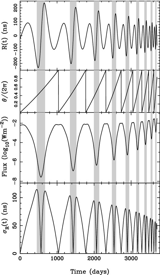
Properties of GW signal and induced ToA variations for a binary SMBH with eccentricity 0.8, orbital period (at the Earth) of 3.1 yr at the starting time, component masses M1 = 1010 M⊙ and M2 = 5 × 10⁹ M⊙ and redshift 0.1. The grey shadings in each panel represent the time periods identified as GW bursts. The panels, from the top, are described in turn. First panel: the ToA variations corresponding to the metric perturbations at the Earth, for arbitrary orientation parameters, with the mean subtracted. Second panel: the orbital phase θ, measured from the common line of nodes and periapse. Third panel: the GW flux at the Earth. Fourth panel: the rms-induced pulsar ToA variations, averaged over all orientation parameters. The time coordinate is measured at the Earth. Not all minima in the bottom curve are at a value of zero because of imperfect numerical sampling.
The qualitative properties of σR(t) in Fig. 5 apply to binaries with any component masses, orbital period and eccentricity. That is, there are two peaks per rotation period, separated by less in orbital phase for more eccentric binaries, and separated by half an orbital phase for circular binaries. For a binary specified by |$\boldsymbol {\zeta }$| and z, we integrate the equations for the evolution of the orbit (Peters & Mathews 1963) from zero orbital phase to numerically calculate Rburst as the mean of the first two peaks in σR(t), and Tburst as the time interval between peaks.
We use the distribution of binary SMBHs, |$D_{\boldsymbol {\zeta }}[N(\boldsymbol {\zeta },z)]$|, to calculate the distribution of GW bursts. As described above, this distribution is specified as the number of binaries in discrete bins of width ΔM1, ΔM2, Δz, Δforb and ΔeGW, where the eccentricity bin widths depend on the other parameters. Scaling this distribution by the comoving volume shell between redshifts z − Δz/2 and z + Δz/2 specifies the number of observable binary SMBHs. For parameters at the midpoints of each bin, we calculate Rburst and Tburst. We approximate the burst rate from binaries in a bin as the number of binaries divided by their period observed at the Earth, and record the expected number of bursts in a 10 yr time span.
4.2 Results
Using the distributions of binary SMBHs for w0 = 0.1 and 0.93, we calculated the numbers of GW bursts for different values of the expected maximum level of ToA variations, Rburst, and the duration, Tburst. We depict the distributions of GW bursts in Fig. 6 as the number of bursts per 10 yr observation time, N10, dex−2, in bins of 0.075 dex in Rburst and 0.05 dex in Tburst. We only considered bursts with Rburst ≥ 40 ns and 0.1 ≤ Tburst ≤ 10 yr. An rms ToA variation of 40 ns corresponds to the best-timing precisions currently achieved for millisecond radio pulsars (Hobbs 2013; Osłowski et al. 2013).
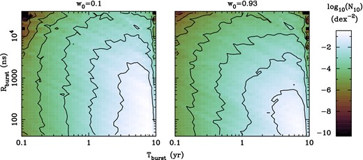
Illustrations of the distributions of GW bursts in the w0 = 0.1 (left) and w0 = 0.93 (right) cases. The shading represents the expected number of bursts in a 10 yr time span, N10, dex−2. The distributions are binned over 0.05 dex in duration and 0.075 dex in amplitude. The contours connect regions at intervals of factors of 10 below the peak.
In total, we predict 0.06 bursts per 10 yr in the w0 = 0.93 case with these strengths and durations, as compared with 0.12 bursts per 10 yr in the w0 = 0.1 case. This difference in the total number of bursts is because of the smaller number of binary SMBHs that we expect to observe if the population is generally more eccentric. However, we note that bursts from low-eccentricity binaries, which will dominate the burst population in the w0 = 0.1 case, may be less detectable than bursts from high-eccentricity binaries. There are proportionally more short-duration bursts in the w0 = 0.93 case than in the w0 = 0.1 case, because larger binary eccentricities result in shorter bursts.
In both cases, the burst distribution is quite heavily skewed towards long bursts, with approximately a factor of 100 more bursts expected with ∼8 yr durations than with ∼1 yr durations. There are also fewer bursts with durations longer than ∼8 yr in both cases. This typical burst duration corresponds to binaries with separations where GW-driven evolution is equivalent to evolution driven by stellar environments.
The typical combined masses of the binary SMBHs that produce GW bursts are ∼1010 M⊙. In Fig. 7, we show the distributions of the combined masses of all binary SMBHs producing the bursts in the distributions in Fig. 6. The distributions are similar in shape, although the distribution for w0 = 0.93 includes relatively more high-mass binaries than the distribution for w0 = 0.1. This is because, in the w0 = 0.93 case, lower mass binaries are less likely to be able to produce strong GW bursts because they are likely to be more eccentric. More eccentric binaries of a given mass and orbital period produce typically weaker bursts (see equation B11 in Appendix B).

The distributions of combined masses (M1 + M2) of binary SMBHs contributing to the GW burst distributions presented in Fig. 6. The solid grey histogram corresponds to the w0 = 0.1 case, and the dashed black histogram corresponds to the w0 = 0.93 case. Both histograms are normalized to the peak of the w0 = 0.1 histogram.
In summary, we find the following.
For bursts with durations between 0.1 and 10 yr, and with expected maximum ToA variations of >40 ns, we predict between 0.06 and 0.12 bursts per 10 yr observation, with lower burst rates corresponding to higher eccentricity binary SMBH populations.
Higher eccentricity binary populations result in relatively more shorter duration bursts than lower eccentricity populations.
However, the burst rate decreases by a factor of 10 per ∼0.4 dex below a duration of ∼8 yr. This also appears to be the most likely duration, with few bursts longer than 8 yr expected.
The burst rate decreases by a factor of 10 per ∼0.8 dex increase in amplitude.
Various uncertainties discussed in Section 3.3 also apply to these calculations. The uncertainty in the galaxy merger rate will also directly correspond to the uncertainty in the GW burst rate (i.e. 0.3 dex). Given that the high-end power-law logarithmic slope of the SMBH mass function in the G11 model is ∼−2, the 0.2 dex uncertainty in the SMBH masses will, to first order, correspond to an uncertainty of 0.4 dex in the merger rate. Therefore, the 1σ uncertainty in the burst rate from the model is approximately 0.5 dex.
To our knowledge, only one study has attempted to predict the properties of GW bursts from a population of eccentric binary SMBHs (Liu et al. 2012). While our modelling methods and definition of GW bursts differ substantially from this work, we agree with these authors that it is unlikely that current PTAs will be able to detect GW bursts from binary SMBHs. The rarity of short GW bursts (lasting around 1 yr) from binary SMBHs suggests that high-cadence PTA observations targeting such bursts are not well motivated.
5 SUMMARY OF RESULTS
We have used a semi-analytic model for galaxy and SMBH formation and evolution (G11) implemented in the Millennium simulation (Springel et al. 2005), augmented with a model for the evolution of binary SMBHs within fixed stellar backgrounds (Sesana et al. 2006; Sesana 2010), to predict the properties of low-frequency GWs from binary SMBHs. We specify the form of a phenomenological distribution of initial binary eccentricities, and consider a selection of cases with differing levels of typical binary eccentricity.
Our quantitative results are uncertain due to a variety of factors. The range of initial binary eccentricity distributions that we consider corresponds to a 0.4 dex variation in the characteristic strain spectrum at low frequencies. Moreover, uncertainties in the tuning of the G11 model provide another 0.2 dex of uncertainty in the spectrum at all frequencies. There is also uncertainty in our estimate of the binary SMBH distribution predicted by the G11 model, in particular for the most massive binaries. Finally, while the G11 model is likely to provide a satisfactory representation of the merger rate of massive, low-redshift galaxies, the binary evolution model that we use may overestimate binary hardening caused by stellar interactions.
Our specific findings are as follows.
The expected characteristic strain spectrum of the GW background from binary SMBHs will turn over from the standard hc(f)∝f− 2/3 power law at a frequency up to 2 × 10⁻⁸ Hz. The turn-over frequency depends on the efficiency of stellar interactions in extracting energy and angular momentum from binary SMBHs, as well as the typical binary eccentricities at formation.
The nature of the spectrum at frequencies below the turn-over frequency is extremely uncertain, and depends on the numbers of massive (M1 + M2 ≥ 1010 M⊙) binaries and on binary eccentricities. The most massive binary SMBHs predominantly produce the lowest frequency parts of the spectrum, and their numbers depend strongly on the strength of their coupling to their environments. The spectrum will be attenuated if binaries with typically larger eccentricities are present.
The most massive eccentric binaries will very rarely produce GW bursts detectable in pulsar timing data. A larger eccentricity binary population will produce fewer bursts that are typically shorter and weaker. Our results suggest that GW bursts from binary SMBHs do not provide viable targets for PTA observations.
We emphasize a set of key implications of our work for PTAs.
Given the expected low-frequency turn-over in the GW characteristic strain spectrum, along with the large uncertainty in the signal at these frequencies, the increase with time of PTA sensitivities to a GW background from binary SMBHs will not be as strong as currently thought.
Short-duration, strong GW bursts from eccentric binary SMBHs are unlikely to occur during typical PTA data set lengths.
PTA data analysts cannot assume hc(f)∝f− 2/3 when searching for a GW background from binary SMBHs. Indeed, model-independent searches cannot assume any particular spectral shape.
Model-dependent searches and constraints need to carefully account for the uncertainty in model predictions.
6 CONCLUSIONS
In this paper, we predict both the GW background characteristic strain spectrum and the distribution of strong GW bursts from eccentric binaries. At a GW frequency of (1 yr)−1, we predict a characteristic strain of 6.5 × 10− 16 < hc < 2.1 × 10− 15 with approximately 68 per cent confidence.
Accelerated binary evolution driven by three-body stellar interactions causes the characteristic strain spectrum to be diminished with respect to a hc(f)∝f− 2/3 power law at f ≲ 2 × 10⁻⁸ Hz. At these low frequencies, the signal is further attenuated if binary SMBHs are typically more eccentric at formation. The low-frequency signal may be dominated by a few binaries with combined masses (M1 + M2) greater than 1010 M⊙, to a larger extent than predicted in the circular, GW-driven case (Ravi et al. 2012). Numerous uncertainties, however, affect our results. These include observational uncertainties in parameters of our model, and theoretical uncertainties in the efficiency of coupling between binary SMBHs and their environments.
We also expect between 0.06 and 0.12 GW bursts that produce >40 ns amplitude ToA variations over a 10 yr observation time. Larger typical binary eccentricities at formation will result in fewer events than if binaries are less eccentric at formation. These bursts are caused by binary SMBHs with combined masses of ∼1010 M⊙, and typically last ∼8 yr. Shorter, stronger bursts are significantly less likely, as are longer bursts.
Upcoming radio telescopes with extremely large collecting areas, such as the Five-hundred-metre Aperture Spherical Telescope (FAST; Li, Nan & Pan 2013) and the Square Kilometre Array (SKA; Cordes et al. 2004) are likely to significantly expand the sample of pulsars with sufficient timing precision for GW detection as compared to current instruments. PTAs formed with FAST and the SKA will hence be sensitive to a stochastic GW signal at much higher frequencies than current PTAs, which is desirable given the results we present.
The mechanism by which binary SMBHs are driven to the GW-dominated regime must involve some form of binary–environment coupling. Hence, independent of the exact model, there will always be some low-frequency attenuation of the GW signal relative to the circular, GW-driven binary case. Our results indicate that this attenuation occurs within the PTA frequency band. However, the strength of the binary–environment coupling is quite uncertain, and we urge future work on this topic. Finally, as also emphasized in previous works (Enoki & Nagashima 2007; Sesana 2013b), constraining or measuring the spectrum of the GW background at a number of frequencies would provide an excellent test of models for the binary SMBH population of the Universe.
The authors thank Alberto Sesana, Sarah Burke-Spolaor, Yuri Levin, Simon Mutch, Paul Lasky and Jonathan Khoo for useful discussions. VR is a recipient of a John Stocker Postgraduate Scholarship from the Science and Industry Endowment Fund, and JSBW acknowledges an Australian Research Council Laureate Fellowship. The Millennium and Millennium-II simulation data bases used in this paper and the web application providing online access to them were constructed as part of the activities of the German Astrophysical Virtual Observatory. This work was performed on the swinSTAR supercomputer at the Swinburne University of Technology.
We refer to this as the ‘circular, GW-driven case’ throughout the paper.
See Gaddum (1945) for a discussion of the ubiquity of log-normal distributions in nature.
REFERENCES
APPENDIX A: TESTING OUR IMPLEMENTATION OF A BINARY SMBH EVOLUTION MODEL
In the main text, we use the results of Sesana et al. (2006) and Sesana (2010) (hereafter collectively referred to as S06) to model the evolution of binary SMBHs in fixed stellar backgrounds for separations less than aH (see equation 6). S06 numerically solved three-body scattering problems for binary SMBHs interacting with stars on radial, intersecting orbits drawn from a spherically symmetric, fixed distribution, and provided fitting formulae for the binary hardening and eccentricity growth rates as functions of binary properties. We use these fitting formulae to evolve binary SMBH orbits as described in Section 2.3.
Here, we compare this method of evolving binary SMBHs with recent N-body simulations of binary SMBH evolution in merging galaxies of various mass ratios and stellar density distributions (Khan et al. 2012, hereafter K12). K12 simulated the mergers of spherical galaxies with various mass ratios, power-law stellar cusp density profiles with various indices, with typical approach trajectories from cosmological simulations. The SMBHs were traced until separations close to, and in some cases beyond, where the GW-driven orbital decay dominated the orbital decay caused by three-body stellar interactions. By extrapolating the binary orbits assuming constant stellar-driven hardening rates and eccentricities, K12 estimated binary semimajor axes, aK12, below which GW-driven evolution dominated. The accuracy of these extrapolations was confirmed using a selection of simulations including post-Newtonian corrections to the binary SMBH orbits.
Here, we take the final eccentricities and semimajor axes of the binaries in each of the scenarios considered by K12 for which aK12 was estimated, and evolve the binaries using the binary evolution model of S06 to estimate an equivalent quantity to aK12, aS06. We list the ratios aS06/aK12 in Table A1 both without (column 4) and with the binary eccentricity held fixed (column 5) for each relevant scenario of K12. The cusp density profile indices, γ, and the galaxy and SMBH mass ratios, q, are given in columns 2 and 3, respectively.
| Model | γ | q | |$\frac{a_{{\rm S06}}}{a_{{\rm K12}}}$| | |$\frac{a_{{\rm S06}}}{a_{{\rm K12}}}$| (fixed e) |
|---|---|---|---|---|
| A1 | 0.5 | 0.1 | 0.51 | 0.47 |
| A2 | 0.5 | 0.25 | 0.72 | 0.53 |
| A3 | 0.5 | 0.5 | 0.62 | 0.57 |
| A4 | 0.5 | 1.0 | 0.68 | 0.65 |
| B1 | 1.0 | 0.1 | 0.58 | 0.36 |
| B2 | 1.0 | 0.1 | 0.74 | 0.38 |
| B3 | 1.0 | 0.1 | 0.87 | 0.41 |
| B4 | 1.0 | 0.1 | 0.93 | 0.47 |
| D1 | 1.75 | 0.1 | 0.72 | 0.41 |
| D2 | 1.75 | 0.1 | 0.68 | 0.44 |
| D3 | 1.75 | 0.1 | 0.62 | 0.48 |
| D4 | 1.75 | 0.1 | 0.63 | 0.51 |
We find |$0.1<\frac{a_{{\rm S06}}}{a_{{\rm K12}}}<1$| in all cases. This implies that the S06 model that we use in our work has stronger stellar-driven binary evolution than the K12 model. We also have smaller ratios |$\frac{a_{{\rm S06}}}{a_{{\rm K12}}}$| when we hold the binary eccentricities fixed. This is because the binary eccentricities invariably grow when allowed to evolve, and lower eccentricities imply smaller GW-driven hardening rates. While an intuitive explanation of the difference between the S06 and K12 models is difficult to attain, the K12 work involves a more sophisticated, and possibly more realistic, treatment of the distribution of stellar orbits in the cores of merged galaxies than the S06 work. Given forb∝a− 3/2 (equation 9), a difference of a factor of 2 in the semimajor axes at which binary SMBH evolution begins to be GW dominated corresponds to a difference of a factor of 23/2 (∼ 0.45 dex) in orbital frequency.
