


Abstract
We present new 3D numerical simulations for Kepler's supernova remnant. In this work we revisit the possibility that the asymmetric shape of the remnant in X-rays is the product of a Type Ia supernova explosion which occurs inside the wind bubble previously created by an AGB companion star. Due to the large peculiar velocity of the system, the interaction of the strong AGB wind with the interstellar medium results in a bow shock structure. In this new model we propose that the AGB wind is anisotropic, with properties such as mass-loss rate and density having a latitude dependence, and that the orientation of the polar axis of the AGB star is not aligned with the direction of motion. The ejecta from the Type Ia supernova explosion is modelled using a power-law density profile, and we let the remnant evolve for 400 yr. We computed synthetic X-ray maps from the numerical results. We find that the estimated size and peculiar X-ray morphology of Kepler's supernova remnant are well reproduced by considering an AGB mass-loss rate of 10−5 M⊙ yr−1, a wind terminal velocity of 10 km s−1, an ambient medium density of 10−3 cm−3 and an explosion energy of 7 × 1050 erg. The obtained total X-ray luminosity of the remnant in this model reaches 6 × 1050 erg, which is within a factor of 2 of the observed value, and the time evolution of the luminosity shows a rate of decrease in recent decades of ∼2.4 per cent yr−1 that is consistent with the observations.
1 INTRODUCTION
Kepler's supernova remnant (SNR; SN 1604, G004.5+06.8, V 843 Ophiuchi) is one of the few supernova events in our Galaxy that have been observed in historical times. Just above 400 years old, this young remnant has been observed by a multitude of scientific instruments in different spectral bands over the past decades: several VLA radio observations (e.g. Reynoso & Goss 1999; DeLaney et al. 2002), a submillimetric dust study by Morgan et al. (2003), optical imaging and spectroscopy using both ground-based telescopes and the Hubble Space Telescope (e.g. Blair, Long & Vancura 1991; Green et al. 1997; Sollerman et al. 2003; Sankrit et al. 2008), Spitzer (Blair et al. 2007) and near-infrared (Gerardy & Fesen 2001) imaging and spectroscopy, as well as multiple X-ray studies using the space telescopes Einstein (White & Long 1983), ROSAT (Predehl & Schmitt 1995), ASCA (Kinugasa & Tsunemi 1999), XMM–Newton (Cassam-Chenaï et al. 2004) and Chandra (e.g. Bamba et al. 2005; Reynolds et al. 2007).
The observations across multiple wavelengths reveal a complex morphology which is prominently asymmetrical. In Fig. 1 we present a radio image at 1.42 GHz (Fig. 1a, left panel) reprocessed from archival VLA1 observations, and an X-ray image from the Chandra catalogue (Fig. 1b, right panel) in the band 2–10 keV. In both bands, the remnant appears as an incomplete shell which is considerably brighter to the North-west and displays two protuberances (‘ears’) that are roughly aligned with the Southeast–North-west axis (Dickel et al. 1998). Another remarkable feature is a curved bar-like structure that spans across the remnant roughly from its South to North limbs. The diameter of the shell is approximately 3.3 arcmin (Blair 2005). In the optical (e.g. Sankrit et al. 2008), the emission comes from dense, knotty structures (radiative shocks) with an excess of nitrogen, and from thin Hα filaments (non-radiative shocks). Overall, the optical emission roughly corresponds to the bright NW regions in radio and X-rays.
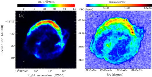
(a) VLA image of Kepler's SNR at 1.4 GHz. The beam is 7.6 × 5.3 arcsec, with a position angle of 39.°8 (bottom left). The intensity scale, in mJy beam−1, is displayed in the bar at the top. (b) Chandra catalogue X-ray image of Kepler's SNR in the band 2–10 keV.
The nature of Kepler's supernova explosion has been debated a lot. The relatively high Galactic latitude of the remnant (l = 6| $_{.}^{\circ}$|8) and the reconstructed light curve based on historical observations (Baade 1943) initially prompted a Type Ia identification. However, its high spatial motion away from the Galactic plane and the presence of nitrogen in optical observations (which is usually associated with stellar winds) challenged this view, suggesting a core-collapse scenario instead (e.g. Borkowski, Sarazin & Blondin 1992). Nevertheless, X-ray studies have generally provided evidence in favour of the initially suggested Type Ia scenario. In particular, the large iron abundance (Kinugasa & Tsunemi 1999; Cassam-Chenaï et al. 2004), which is consistent with Type Ia supernovae, as well as the absence of a neutron star (Reynolds et al. 2007), which would be an additional indication of a core-collapse event, has led us (Reynolds et al. 2007) to conclude that Kepler's SNR is the result of a Type Ia explosion. Furthermore, the hydrodynamical models of Borkowski et al. (1992) and Velázquez et al. (2006) found that a Type Ia origin produces numerical results that are a closer match to the observations.
The most likely explanation for the asymmetric brightness of the northwestern region is that the medium in which the ejected material expands is inhomogeneous. Since strong density gradients are not expected at such high altitude above the Galactic plane, this suggests that the progenitor system had an important role in shaping the circumstellar medium (CSM). Van der Bergh et al. (1977) analysed the proper motions of optical knots within the nebula and determined that the progenitor must have had a high peculiar velocity relative to the ambient medium. Using more recent data, Bandiera & van den Bergh (1991) determined this velocity to be around 280 km s−1.
This prompted the idea that the northwestern region is the product of the interaction between the supernova shock wave and the bow shock structure produced by the stellar wind of an evolved star as it travels through the ambient medium. Bandiera (1987) and Borkowski et al. (1992) investigated this ‘runaway progenitor’ hypothesis in depth and found that it can explain not only the brightness of the northwestern region, but also the absence of a sharp limb on the southern edge. This idea can also be reconciled with a Type Ia explosion if the progenitor was in fact a symbiotic binary system: the wind of the AGB donor star blows a bubble in the CSM in which the white dwarf companion later explodes. The 2D numerical models of Chiotellis, Schure & Vink (2012) explored this specific scenario in great detail and obtained results that quite accurately reproduce the X-ray morphology and kinematics of the remnant. Burkey et al. (2013) improved the results by including in the 2D simulation an equatorial wind from the AGB donor. The authors were able to isolate the shocked CSM from the SN ejecta by applying a Gaussian mixture model to Chandra spectral data and found that the shocked CSM is coincident with the bright northern rim and parts of the central bar.
The presence of asymmetries such as bipolar outflows in many planetary nebulae suggests that the wind ejected during the AGB or post-AGB phase must have some degree of anisotropy (e.g. Mellema 1995; Gruendl et al. 2006). Moreover, anisotropic AGB winds have been detected through high-resolution molecular line observations (e.g. Bieging & Tafalla 1993; Lucas et al. 1995). While many 2D models assume that the AGB wind and resulting SNR expansion are axially symmetric, this is not necessarily the case.
The main goal of this work is to explore a range of fully 3D numerical models that might explain the X-ray appearance of Kepler's SNR based on the runaway symbiotic binary scenario, introducing a source of asymmetry by considering a possible anisotropy in the AGB wind. The paper is organized as follows. In Section 2, we discuss the details of the 3D model. The details of the numerical simulations are then explained in Section 3. The results are presented in Section 4 and discussed in Section 5. Finally, we give our conclusions in Section 6.
2 THE MODEL
In order to explain the asymmetric features of Kepler's SNR, we have explored a numerical model that is based on Bandiera's runaway progenitor scenario, but with the additional consideration that the AGB wind is not isotropic. That is, the model assumes that the SN explosion occurred inside an asymmetric CSM density distribution produced by the companion AGB star before the mass-transfer resulting in a Type Ia explosion was complete. The peculiar structure of this wind bubble is shaped by two factors: (1) the bow shock produced by the high-velocity motion of the AGB star through the ambient galactic medium, and (2) the latitude dependence of the properties (density and terminal velocity) of the AGB wind. The combination of these two elements yields a complex CSM which determines the appearance of several striking morphological features of the expanding SNR.
The proper motion of the AGB star results in the characteristic ‘cometary’ double-shock structure consisting of a forward bow shock which compresses the interstellar medium (ISM), an inner reverse shock where the stellar wind is slowed down and compressed, and a contact discontinuity separating shocked ISM from shocked stellar wind. The properties of this structure are determined by four parameters: the mass-loss rate of the stellar wind, |$\dot{M}$|, the terminal velocity of the wind, vw, the peculiar velocity of the AGB star through the ISM, v⋆, and the mass density of the ISM, ρ0.
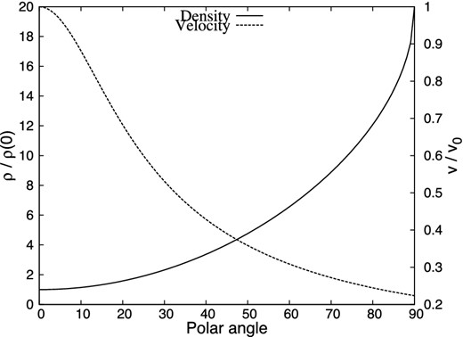
Density (continuous line) and velocity (dashed) profiles as a function of polar angle (0° at the pole and 90° at the equator) for ξ = 20, normalized to the values at the pole.
This choice of density and velocity guarantees that the ram pressure of the wind, ρv2, is isotropic. The scaling constant A can be computed by associating the mass-loss rate of the wind to the integral of the density and velocity; for this particular choice of the function f(θ) and an equator-to-pole density ratio of ξ = 20, Raga et al. (2008) obtained |$A=0.389\dot{M}_{\rm w}/(4 \pi v_{{\rm pole}})$|.
Finally, we allowed the polar axis to be tilted by an angle ϕ. We have found that a tilt angle of ϕ ≈ 70° produces satisfactory results. This eliminates any remaining symmetry in the problem and thus requires a fully 3D simulation.
3 NUMERICAL SIMULATIONS
3.1 Numerical method
We performed numerical simulations using the 3D hydrodynamical adaptive mesh refinement Walicxe3D code developed by J.C. Toledo-Roy. The code is an extension to 3D of the Walicxe code (Esquivel et al. 2010), and has been used to model the multiple-ring SNR G352.7-0.1 (?).
The code solves equations (5)–(7) by means of a finite-volume, conservative, second-order Godunov upwind scheme. The Riemann solver uses a second-order Runge–Kutta method for the time integration and a linear spatial reconstruction of the primitive variables at the interfaces, including a slope limiter in order to suppress spurious oscillations. The numerical fluxes are calculated using the HLLC solver, which is a contact discontinuity-capturing modification by Toro, Spruces & Speares (1994) of the original HLL solver (Harten, Lax & van Leer 1983). Since the cooling region behind the main shock cannot be resolved at typical grid resolutions, the code does not limit the integration time-step to the cooling time-scale, employing only the dynamical time-scale (through the standard Courant–Friedrichs–Lewy condition) to limit the time-step size.
For specific details of the code, such as those related to the numerical integrator, the adaptive mesh algorithm, or the parallelization scheme, see the appendix of Esquivel et al. (2010), where the precursor 2D version of Walicxe3D is described.
The code also includes radiative cooling as a source term in the energy equation, equation (7), in which Λ(T) is a parametrized cooling function and n is the gas number density. The cooling function Λ(T) is taken as a tabulated coronal equilibrium curve (Dalgarno & McCray 1972), which is plotted in fig. 2 of Toledo-Roy et al. (2009). This cooling function is well suited for temperatures above 104 K. Below this threshold, it is turned off, and above 108 K it is substituted by a Λ ∝ T1/2 law (corresponding to the free–free regime). It is worth mentioning that the temperature used in the cooling calculation is computed by assuming that gas above 104 K is fully ionized. This is achieved by using the correct mean atomic mass of μ = 0.6 where appropriate, instead of the value for neutral gas.
3.2 Calculation of the thermal X-ray emission
In order to further compare the results of the numerical simulations with the observations, we have also calculated synthetic thermal X-ray maps by integrating the X-ray emission coefficient jν(n, T). The coefficient was calculated (in the low density regime) as |$j_{\nu }(n,T)=n_{\rm e}^2 \xi (T)$|, where ne and T are the electronic density (assumed to be ne ≈ nH) and temperature obtained from our numerical simulations, while ξ(T) is a function smoothly varying with temperature. The function ξ(T) was computed for the range 0.15–8 keV and standard solar metallicity using the chianti atomic data base and its associated idl software (Dere et al. 1997; Landi et al. 2006). It should be noted that this calculation assumes ionization equilibrium, which might not reflect the true ionization state of the plasma. While a full non-equilibrium treatment is feasible in 1D simulations (e.g. Badenes et al. 2003; Kosenko et al. 2011), it can be computationally expensive for the 3D case. However, Hughes & Helfand (1985) have found that the differences introduced by the simplifying assumption of ionization equilibrium are only important at low energies (less than 2 keV); in this work we study the X-ray emission in the 2–10 keV range.
In the calculation of these emission coefficients, we have considered the high metal abundances found in Kepler's SNR (see e.g. Cassam-Chenaï et al. 2004, Reynolds et al. 2007). Specifically, we have used the values of the two-component thermal plasma model of Kinugasa & Tsunemi (1999), which are reported in the Chandra Supernova Remnant Catalogue. These include specific metal enhancements for Si and S. The effects of considering additional metal enhancements are discussed in Section 5.
3.3 Initial conditions: precursor AGB wind
The code is first used to compute the evolution of the stellar wind originating in the AGB companion star. In order to do this, we have initialized the computational domain, which spans a box of 12 × 12 × 12 pc, with a uniform medium of number density n0 and temperature of 104 K.
The anisotropic wind source is fixed at the centre of the box and in order to represent the effects of the star's proper motion through the ISM, an inflow condition is imposed on the wall at the +z face having a velocity of v⋆ = 280 km s−1 and moving towards the −z direction. The boundary conditions on the rest of the walls are transmissive. The wind is made anisotropic as explained in Section 2. In Fig. 3 we show a schematic representation of the initial setup.
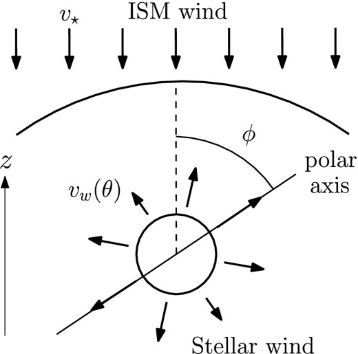
A schematic representation of the initial setup for the AGB wind phase.
In this work we have explored four numerical models using different combinations of the mass-loss rate (|$\dot{M}_{\rm w}$|) and terminal velocity at the pole (vpole) of the AGB wind. These values range from 3 × 10⁻⁶ to 1 × 10⁻⁵ M⊙ yr−1 for the mass-loss rate and from 10 to 20 km s−1 for the wind terminal velocity. The specific values for each model are given in Table 1.
Wind parameters for the numerical models. The following parameters are common to all models: v⋆ = 280 km s−1, T = 1000 K and μ = 1.3.
| Parameter | Model A | Model B | Model C | Model D |
|---|---|---|---|---|
| |$\dot{M}$| (M⊙ yr−1) | 7 × 10⁻⁶ | 10−5 | 3 × 10⁻⁶ | 4 × 10⁻⁶ |
| vpole (km s−1) | 15 | 10 | 20 | 12 |
| n0 (cm−3) | 10−3 | 10−3 | 6 × 10⁻⁴ | 5 × 10⁻⁴ |
| r0 (pc) | 2.06 | 2.01 | 2.01 | 1.97 |
| Mejected (M⊙) | 3.5 | 5.0 | 1.5 | 2.0 |
Since |$\dot{M}_{\rm w}$| and vpole are fixed in each model, and we have used a constant value for v⋆ across all models, we have in each case selected the ISM number density n0 so that an equivalent isotropic stagnation distance r0 of ∼2 pc is obtained. The specific values for the ISM density in each case are also reported in Table 1. While it is hard to directly assess the density in the region surrounding Kepler's SNR, these values fall in the range n0 ∼ 10−4–10−3, which is typical of the hot ionized component of the ISM (McKee & Ostriker 1977). This component might very well extend into the remnant's galactic latitude. These values are also in agreement with those used in the numerical models of Borkowski et al. (1992) and Chiotellis et al. (2012).
The AGB wind is then left to evolve for an integration time large enough that the bow shock structure would in principle arrive at a quasi-steady state. This time can be set by computing the flow time-scale defined in Section 2. Using the values l ∼ 2 pc (the distance between the wind source and bow shock) and vpole ∼ 10 km s−1 (the lowest value in all models), we obtain that the flow time-scale is no larger than tflow ∼ 200 kyr across all models. Thus, a total integration time of 500 kyr guarantees that a steady state should be approximately reached. This is also within the estimated lifetime of the AGB star. However, while the position of the bow shock does reach an approximate steady state, the contact discontinuity becomes noticeably Kelvin–Helmholtz unstable in all models at around 200 kyr, producing a complex time-dependent flow in the region inside the bow shock.
The density cuts of Fig. 4 show the evolution of the AGB wind for Model B at four time snapshots. The typical four-region structure produced by the interaction of the AGB wind with the ISM can be seen divided by three discontinuities in the flow. The outermost one is the bow shock, where the ISM is shocked and compressed. This shock reaches a minimum distance from the wind source of about 3 pc in the final snapshot (except for model C, in which the bow shock extends to about 2 pc). Farther in, towards the wind source, a strong density jump is encountered marking the contact discontinuity that separates shocked ISM from shocked stellar wind material. Finally, the shocked stellar wind is divided from the free-streaming wind by the termination shock, across which a final density jump yields to the unperturbed stellar wind originating in the central source.
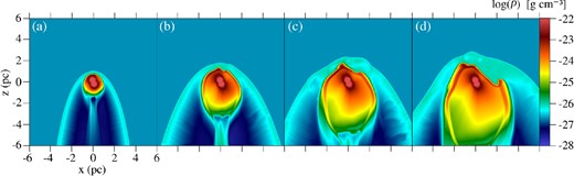
Evolution of the AGB wind for Model B. Shown here are xz cuts at y = 6 pc of the mass density for the integration times (a) 50 kyr, (b) 200 kyr, (c) 350 kyr and (d) 500 kyr. The logarithmic scale is the same for all panels and is given in g cm−3.
The shear between the flows at the contact discontinuity becomes susceptible to the Kelvin–Helmholtz instability at about 200 kyr, thus producing a complex flow morphology that prevents the wind structure from achieving a true steady state. Thus, the predicted stagnation distance of 2 pc is only approximately reached. This complex wind bubble will strongly influence the evolution and morphology of the subsequent SNR.
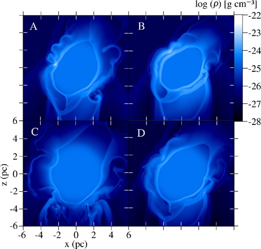
In Fig. 5 we compare the final wind bubble structure of all four models at t = 500 kyr. Models A, B and D display a qualitatively similar structure, with a clear wind bubble and a well-defined, albeit somewhat Kelvin–Helmholtz unstable, contact discontinuity. Model C, however, exhibits a much more turbulent wind structure downstream of the central wind source. The main difference between this model and the rest is that the wind terminal velocity is higher, 20 km s−1, which would result in a stronger shearing between the flows at the contact discontinuity, thus enhancing the instability and producing the observed turbulent structure.
A comparison of the AGB wind structures at t = 500 kyr for all four models. Shown here are xz cuts at y = 6 pc of the mass density. The model is indicated by the letter in the upper left corner. The logarithmic scale is the same for all panels and is given in g cm−3.
Since the typical mass-loss rates of AGB stars can be as high as 10−5 M⊙ yr−1 while the AGB phase might last as much as 1 Myr (Vassiliadis & Wood 1993), we have checked that the total mass ejected by the AGB wind in all models does not surpass ∼5 M⊙ by the time we introduce the SNR into the simulation. The mass ejected by the models is reported in the last row of Table 1, with model B having the highest value.
3.4 Initial conditions: supernova remnant
After letting the wind bubble evolve for each model, the supernova explosion is imposed in the computational domain by injecting E = 7 × 1050 erg and M = 1.4 M⊙ into a spherical region at the centre of the domain. This choice of the energy in the explosion was made in order to match the observed linear size of the object deduced from the assumed distance to Kepler's SNR, which we consider to lie in the lower range of 3.4–6.4 kpc (with a ‘nominal’ value of ∼5 kpc) as found by Reynoso & Goss (1999) based on H i absorption. X-ray observations with HESS (Aharonian et al. 2008) as well as previous hydrodynamical simulations (Patnaude et al. 2012; Chiotellis et al. 2012) have shown that in this case the radius of the forward shock requires the explosion to be subenergetic.
Since the early evolution of SNRs is sensitive to the detailed kinematics of the SN ejecta, we have followed the prescription of Jun & Norman (1996) for SN Ia ejecta. Here, 3/7 of the ejecta mass are injected into the outer portions of the spherical region with a power-law density profile ρ ∼ r−7, while the remaining 4/7 form an inner ‘core’ of constant density ρc. The explosion energy is distributed as 95 per cent kinetic energy with the rest as thermal energy, and the velocity profile is assumed to increase linearly with radius, reaching a value v0 at the edge of the region. The radius rc and density ρc of the inner core, as well as the velocity v0 at the edge of the ejecta region, can be computed in terms of the explosion energy E and the total mass M and radius R of the SN ejecta [see equations (1)– (3) of Jun & Norman (1996)].
While it is not possible to predict analytically the expansion of the SNR in the asymmetric bubble left behind by the AGB wind, we do not expect the results to be substantially different from those obtained by considering an isotropic wind source of comparable momentum flux. However, since there is still some degree of uncertainty in the distance to Kepler's SNR, the physical radius of the remnant is poorly known. The full range of distance estimates produces a radius in the range 1.5–5.1 pc, with the ‘midrange’ value of 5 kpc yielding a radius of 2.5 pc. It is therefore difficult to place an observational restriction on the size of the remnant obtained in the simulations. As is shown below, the remnant indeed reaches a size of 2–3 pc in the simulations.
As discussed above, the size of Kepler's SNR is poorly determined. In contrast, its age is very precisely known, since the supernova was famously observed by Johannes Kepler in 1604. This implies that at the time of the Chandra X-ray observations in 2000 and 2006 (Vink 2008), the age of the SNR was 396 and 402 years, respectively. Since our goal is to calculate and compare synthetic X-ray observations, we let the SNR evolve for 400 years in the simulation in all models.
4 Results
The density maps in Fig. 6 show the evolution of the SNR of Model B at t = 50, 200, 300 and 400 years after the explosion. In this model, the expanding shockwave reaches and penetrates the termination shock of the wind at t ≈ 50 yr. This produces an important blowout of part of the remnant that rapidly expands into the low-density region between the contact discontinuity and the bow shock, subsequently piercing into the ISM at around 150 yr. By the end of the simulation, this blowout has grown to more than 6 pc in size in the ISM. The shock compression increases the temperature of this material to 109 K, but its density remains rather low (≲10−26 g cm−3) compared to densities seen elsewhere in the remnant. As will be shown below, this material has negligible X-ray emissivity and thus does not play any role in the observed shape of the remnant.
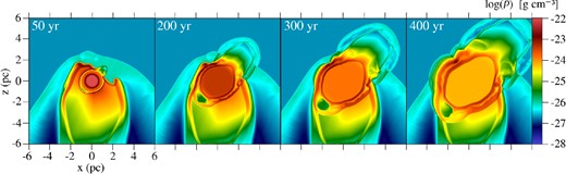
Evolution of the SNR for Model B. Shown here are xz cuts at y = 6 pc of the mass density corresponding to SNR ages of 50, 200, 300 and 400 yr. The logarithmic scale is the same for all panels and is given in g cm−3.
Other parts of the remnant expand mostly into the high-density wind bubble. The wind material is swept up by the blastwave producing a dense (as high as 10−23 g cm−3 in some areas) asymmetric shell that reaches around 2–3 pc in radius, consistent with the approximate observational size of the remnant if the distance is taken to be around 5 kpc.
The expansion parameter, defined as m ≡ v/(R/t) where v is the shock velocity at radius R and t is the age of the remnant, varies in the dense shocked regions of Model B in the range between m ≈ 0.4, which is the asymptotic value in the Sedov–Taylor phase, and m ≈ 0.8. This is consistent with the average value found from X-ray observations, m ≈ 0.6 (Vink 2008).
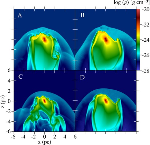
Fig. 7 shows a comparison of the final density maps of all models. The evolution is generally qualitatively similar to that described for Model B, except for the overall size of the structure produced, which is seen to depend on the density of the wind bubble (compare the panels of Fig. 5). Model B has the densest wind bubble of all models and the shock compression by the SN blastwave produces the largest density values.
Comparison of the mass density for the four models at t = 400 yr (xz cuts at y = 6 pc). The logarithmic scale is the same for all panels and is given in g cm−3. The model is indicated in each panel by the letter in the upper left corner.
Since the main goal of this work is to directly compare the models with the observations, we have generated synthetic X-ray maps from the simulation data. Fig. 8 shows the calculated X-ray emission in the range 2–10 keV (similar to the energy range of the Chandra observations). The four rows of the figure correspond to each of the four models A, B, C and D (which are also indicated by the letter in the upper left corner). Interstellar absorption has been included in the calculation of the X-ray coefficients using the column density value of 5 × 1021 cm−2 reported by Reynoso & Goss (1999) for the ‘midpoint’ distance of ∼5 kpc.
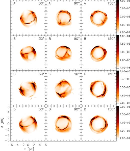
Synthetic X-ray maps in the range 2–10 keV. The model is indicated in each panel with the letter in the upper left corner, while the number in the upper right corner indicates the rotation angle around the z-axis (see text). The linear scale given to the right is the same for the panels corresponding to each model. The horizontal and vertical axes are the same for all panels, with distances given in pc as shown in the bottom left panel.
In order to generate these maps, the z-axis of the computational domain, which is aligned with the direction of motion of the progenitor system relative to the ISM, was first tilted towards the observer at an angle of 35° with respect to the line of sight. This was done so that the orientation of the object coincides with the direction of the velocity of the system determined from the tangential-to-radial velocity ratio of optical knots by Bandiera & van den Bergh (1991).
Additionally, in order to account for the remaining rotational degree of freedom, the resulting coordinate system was rotated a second time around the new vertical axis in steps of 10°, from 0° to 180°. In the figure, we show maps for 30°, 90° and 150° (indicated in the upper right corner of each panel), which adequately sample the full range of maps generated in this manner.
We have also computed the total X-ray luminosity LX of the remnant for each model and the mass of the emitting gas, the latter defined as the mass of the gas with temperature higher than 106 K. The results are reported in Table 2. The time evolution of the total X-ray luminosity is plotted for all models as thick continuous lines in Fig. 9. The luminosity in the first decades of the simulation decreases as the remnant expands into the wind of the AGB. At around 50–100 yr, the shockwave reaches the dense region at the termination shock of the wind and the luminosity increases substantially, reaching a peak value at around 200–250 yr. After that, the luminosity decreases gradually until the present age of the remnant is reached. For model B, the decrease in past decades is around 2.4 per cent per decade, which is consistent with observational (Hughes 1999) and numerical results (Velázquez et al. 2006).

Time evolution of the total X-ray luminosity for the four models. The thick continuous lines correspond to emission coefficients computed using the metal enhancements of Kinugasa & Tsunemi (1999), while the thin dashed lines were obtained with a higher metallicity of Z = 3 solar (see text). The letter label near each pair of curves indicates the model.
Total X-ray luminosity (LX) and mass of the X-ray emitting gas (MX) for all four models at t = 400 yr. The lower luminosity values (second row) were obtained assuming a metallicity Z = 3 solar (see text). The mass of X-ray emitting gas is the same in both cases.
| Quantity | Model A | Model B | Model C | Model D |
|---|---|---|---|---|
| LX (1034 erg s−1) | 2.0 | 5.7 | 0.44 | 1.2 |
| 2.8 | 8.1 | 0.64 | 1.7 | |
| MX (M⊙) | 2.4 | 3.5 | 1.6 | 1.9 |
| Quantity | Model A | Model B | Model C | Model D |
|---|---|---|---|---|
| LX (1034 erg s−1) | 2.0 | 5.7 | 0.44 | 1.2 |
| 2.8 | 8.1 | 0.64 | 1.7 | |
| MX (M⊙) | 2.4 | 3.5 | 1.6 | 1.9 |
5 DISCUSSION
By looking at the leftmost column of Fig. 8, corresponding to 30°, we see that all four models depict a somewhat similar overall morphology: a roughly spherical diffuse emission and a bright incomplete ring-like feature seen on the side. This feature is associated with the interaction of the supernova shockwave and the equatorial regions of the AGB wind, where the density is the highest. However, the models differ slightly (particularly model C) in the shape, orientation and completeness of the ring feature. Also, in all cases a clear enhancement of the emission is seen in the direction going roughly from the lower left to the upper right corner of the figures, which coincides with the equatorial region.
As the view is rotated further to an angle of 90°, the ring-like feature superimposes on to the diffuse emission producing interesting morphological features. Particularly, in models B and D this produces an enhancement of the limb on the upper side and a bar-like feature extending from the lower to the upper limb. This feature is strikingly similar to that observed in the X-ray images, especially in model B. Finally, at an angle of 150° the morphology becomes almost entirely ring-like. The overall size of the remnant in all maps is also in close agreement with the observed radius of 2–3 pc.
According to Table 2, the models are subluminous compared to the observed Chandra value of 1.2 × 1035 erg s−1. The highest luminosity value of 5.7 × 1034 erg s−1 is obtained in model B, which is only within a factor of 2 of the observed value for this energy band. Also, the mass of X-ray emitting gas seems to be lower than estimated by Velázquez et al. (2006). Again, model B exhibits the highest value, which is not surprising considering its higher luminosity.
In a recent study based on the data from the Suzaku Observatory, Park et al. (2013) found evidence that Kepler's progenitor probably had a super-solar metallicity (∼ 3 Z⊙), considering the observed Ni to Fe mass ratio. In order to assess the impact that metallicity can have on the X-ray emission, we have also computed the luminosity of the model assuming that all the X-ray emitting gas has a three times solar metallicity (in contrast to the abundances obtained by Kinugasa & Tsunemi 1999). We obtained a ∼40 per cent increase in the luminosity across all models (see the second row of Table 2). For model B, this boosts the value from 5.7 × 1034 to 8.1 × 1034 erg s−1, which is closer to the observed value. The corresponding luminosity time evolution curves are shown as the thin dashed lines in Fig. 9. The time evolution is in each case qualitatively very similar in spite of the luminosity increase.
In view of its morphological features, size and X-ray luminosity, we consider that model B is the one that most successfully explains the origin of Kepler's SNR. In Fig. 10, we show the X-ray map corresponding to this model for a rotation angle of 70° with a colour map and scale similar to the one used in the Chandra image (Fig. 1b).
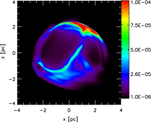
X-ray emission map corresponding to Model B for a rotation angle of 70°, represented with a colour map and scale similar to the Chandra observation (compare to Fig. 1b). The colour bar is given in units of erg s−1 cm−2 sr−1.
Notwithstanding, the total mass ejected during the AGB wind phase in model B (∼5 M⊙) would require a considerably massive (≳6 M⊙) AGB companion. By comparing the predicted chemical yields of AGB stars of Karakas & Lattanzio (2007) with the chemical composition of the shell, Chiotellis et al. (2012) estimate that the AGB companion was probably in the 4–5 M⊙ range. In order to have a total ejected mass of 5 M⊙ and leave behind a stellar core of around 1 M⊙ (Soker et al. 2013), model B requires a slightly more massive AGB companion of around 6 M⊙. It should be noted, however, that this mass requirement is not strict, in the sense that model B may still be viable with a lower total ejected mass during the AGB wind phase, i.e. with a shorter AGB wind phase prior to the explosion. In fact, for a bow shock distance of ∼2 pc and a wind velocity of 10 km s−1, the flow time-scale is around 200 kyr. While this holds for the spherical wind case, in our simulations the wind bow shock structure reaches its approximate final size at around 400 kyr. Imposing the explosion at this time would decrease the total mass ejected by the wind to 4 M⊙, which is compatible with the AGB companion mass estimated by Chiotellis et al. (2012).
Our models do not include the so-called ‘ears’, a characteristic feature of Kepler's SNR. Their apparently symmetrical position with respect to the centre of the object suggests that an additional mechanism may be taking place. Tsebrenko & Soker (2013) recently explored the possibility that these protrusions, which resemble those that are often seen in planetary nebulae, can be attributed to the effect of jets. They propose two scenarios: in the first, jets launched from the white dwarf's accretion disc create opposing lobes on a shell of circumstellar material before the explosion, while in the second the jets are produced when the white dwarf merges with the core of the AGB companion shortly before the explosion. They find that both scenarios are capable of producing the ‘ears’ of the remnant. While it is not clear whether their results extrapolate to the highly complex wind structure produced in our simulations, it will certainly be worth including these jets in our models in a future work.
While in this work we assumed a distance to Kepler's SNR of ∼5 kpc, Patnaude et al. (2012) showed that the amount of 56Ni present in the shell suggests a distance ≳7 kpc. This ∼40 per cent increase in the distance to the remnant would accordingly scale the radius of the forward shock, and thus require the AGB wind bow shock structure in our models to be scaled up as well. One way to achieve this while keeping the same |$\dot{M}$| and vw for each model would be to lower the density n0 of the ambient medium in our simulations by a factor of ∼2 (see equation (1)). For instance, in Model B n0 would have to be decreased to 5 × 10⁻⁴ cm−3, which is still within the characteristic range of the hot ionized component of the ISM. The energy of the explosion would also have to be increased to ≳ 1 × 1051 erg, in agreement with the results of Patnaude et al. (2012). By keeping the same |$\dot{M}$| and vw we would expect the wind bubbles to be structurally similar to those in our current models, and thus the resulting X-ray morphologies to be similar as well. This change in scale would, however, probably increase the X-ray luminosity slightly, as the X-ray emitting region would have a larger volume. This could help achieve a greater agreement between the values obtained in our models and the observations.
6 CONCLUSIONS
In this work we have expanded on the previous numerical studies of Kepler's SNR by performing fully 3D numerical simulations following the AGB wind scenario originally proposed by Bandiera (1987) and recently revisited in 2D simulations by Velázquez et al. (2006), Chiotellis et al. (2012) and Burkey et al. (2013).
In our 3D simulations, the progenitor of Kepler's SNR is a binary system composed by an AGB star with a strong stellar wind and a mass-accreting white dwarf companion. This scenario is consistent with the possible Type Ia nature of Kepler's SN. Due to the system's high peculiar velocity of around 280 km s−1, the interaction of the AGB wind with the ISM produces a wind bubble surrounded by a bow shock.
Additionally, we have considered in our model that the AGB wind is anisotropic, introducing a latitude-dependence in both its terminal velocity and density profile, and have also tilted the polar axis of the AGB star with respect to the direction of motion of the system through the ISM. After the wind bubble is established, we then simulated the detonation of the white dwarf companion by injecting mass and energy into a spherical region, and let the remnant evolve to its present age.
We simulated four models, varying the values of the AGB wind mass-loss rate, terminal velocity and ISM density. The remnant reaches an approximate size of 2–3 pc, except along one of the polar directions in which it blows out of the wind bubble considerably. We obtain expansion parameters in the range 0.4 to 0.8 for the dense regions produced by the interaction of the supernova blastwave and termination shock of the precursor wind.
In order to compare with the observations, we computed synthetic X-ray emission maps, taking into account the estimated direction of motion of the progenitor system with respect to the line of sight and trying several 3D orientations of the simulation data. In all cases, we obtained complex asymmetric X-ray morphologies with a size that is consistent with the observations. Some of the models also exhibit an enhancement of the X-ray emission along parts of the limb, and models B and D also display a central bar-like feature for rotation angles around 90°.
We also calculated total X-ray luminosities and found that most models produce subluminous results with respect to observations, the closest to the observational results being model B, which reaches a luminosity lower than the observations by only a factor of 2. Finally, we analysed the time evolution of the luminosity and recover a decrease in recent decades that is consistent with the observations.
Based on its size, morphology and overall luminosity, we consider model B, for which |$\dot{M}=10^{-5}$| M⊙ yr−1, vpole = 10 km s−1 and n0 = 10−3 g cm−3, to be the model that most successfully explains the origin of Kepler's SNR.
We thank an anonymous referee for insightful comments that improved this work. JCTR, PFV and AE acknowledge support from the CONACyT grants 101356, 101975, 167611, and UNAM DGAPA grants IN105312 and IG100214. EMR is partially supported by CONICET PIP 114-200801-00428. EMR is a member of the Carrera del Investigador Científico of CONICET. We thank Enrique Palacios for maintaining the Diable cluster, where the simulations were performed. chianti is a collaborative project involving George Mason University, the University of Michigan (USA) and the University of Cambridge (UK).
The Very Large Array (VLA) is operated by the National radio Astronomy Observatory, which is a facility of the National Science Foundation, operated under cooperative agreement by Associated Universities, Inc.
