


Abstract
The early X-ray afterglow of gamma-ray bursts revealed by Swift carried many surprises. Following an initial steep decay the light curve often exhibits a plateau phase that can last up to several 104 s, with in addition the presence of flares in 50 per cent of the cases. We focus in this paper on the plateau phase whose origin remains highly debated. We confront several newly discovered correlations between prompt and afterglow quantities (isotropic emitted energy in gamma-rays, luminosity and duration of the plateau) to several models proposed for the origin of plateaus in order to check if they can account for these observed correlations. We first show that the scenario of plateau formation by energy injection into the forward shock leads to an efficiency crisis for the prompt phase and therefore study two possible alternatives: the first one still takes place within the framework of the standard forward shock model but allows for a variation of the microphysics parameters to reduce the radiative efficiency at early times; in the second scenario the early afterglow results from a long-lived reverse shock. Its shape then depends on the distribution of energy as a function of Lorentz factor in the ejecta. In both cases, we first present simple analytical estimates of the plateau luminosity and duration and then compute detailed light curves. In the two considered scenarios we find that plateaus following the observed correlations can be obtained under the condition that specific additional ingredients are included. In the forward shock scenario, the preferred model supposes a wind external medium and a microphysics parameter ϵe that first varies as n−ξ (n being the external density), with ξ ∼ 1 to get a flat plateau, before staying constant below a critical density n0. To produce a plateau in the reverse shock scenario the ejecta must contain a tail of low Lorentz factor with a peak of energy deposition at Γ ≳ 10.
1 INTRODUCTION
Before the launch of the Swift satellite (Gehrels et al. 2004) the afterglow was believed to be the best understood part of gamma-ray burst (GRB) physics, being explained by the energy dissipated in the forward shock formed by the jet impacting the burst environment (Meszaros & Rees 1997; Sari, Piran & Narayan 1998). However, the many surprises of the early X-ray afterglow revealed by Swift – initial steep decay, plateau phase, flares – have considerably complicated the picture (Nousek et al. 2006; O'Brien et al. 2006).
Several mechanisms have been proposed to explain the plateau, the most popular being energy injection into the forward shock (Rees & Meszaros 1998; Sari & Mészáros 2000; Nousek et al. 2006) resulting from a long-lasting activity of the central engine (which could be also responsible for the flares; Zhang et al. 2006) or from a wide distribution of Lorentz factors in the ejecta. Other possibilities include (i) direct emission from a magnetar (e.g. Rowlinson et al. 2013), (ii) coasting of the external blast wave in a wind medium (e.g. Shen & Matzner 2012), (iii) varying microphysics parameters (Granot, Königl & Piran 2006; Ioka et al. 2006), (iv) reverse shock contribution (Genet, Daigne & Mochkovitch 2007; Uhm & Beloborodov 2007). In (i) the end of the plateau corresponds to the spin-down time of the protomagnetar or its collapse to a black hole. Therefore this scenario is mostly promising to explain peculiar plateaus that are followed by a steep decay (temporal index ∼−2 or steeper), while ‘standard’ plateaus (followed by a temporal decay index ∼−1.5) are most likely of afterglow origin; (ii) requires the Lorentz factor of the ejecta to be at most a few tens (so that the coasting phase lasts long enough), which is in severe tension with the minimum Lorentz factor of the ejecta derived from the compactness constraint (e.g. Lithwick & Sari 2001; Hascoët et al. 2012). In this work we focus on cases (iii) and (iv) in connection with the recent discovery of correlations between prompt and afterglow quantities (Dainotti, Ostrowski & Willingale 2011; Dainotti et al. 2013; Grupe et al. 2013; Margutti et al. 2013). We especially want to explore if these correlations can be satisfied by the models and which kind of constraints do they impose.
We first summarize in Section 2 the observational results on the prompt–afterglow correlations and in Section 3 we show that explaining the plateau by late energy injection into the forward shock leads to an ‘efficiency crisis’ for the prompt phase. We then consider in Section 4 the possibility that the microphysics parameters in the forward shock vary during the early afterglow and in Section 5 we explore the alternative model where the afterglow is made by the reverse shock. Our results are discussed in Section 6, which is also the conclusion.
2 THE PROMPT–AFTERGLOW CONNECTION
For events with a measured redshift and a well-defined plateau phase, quantities such as tP – duration of the plateau in the burst rest frame, LP – luminosity at the end of the plateau or EX – energy released in X-rays during the plateau, can be measured together with the isotropic energy in gamma-rays of the prompt phase Eγ,iso. From the samples recently analysed by Dainotti et al. (2011, 2013) and Margutti et al. (2013) some clear correlations appear between prompt and afterglow quantities.1 The plateau luminosity Lp and energy EX increase with Eγ,iso and decrease for larger tp. Since an increase of Lp and EX with Eγ,iso could be expected, we also consider below the ratios Lp/Eγ,iso and EX/Eγ, iso, which, respectively, decrease and barely evolve with increasing tp.
These prompt–afterglow correlations represent potentially important clues to understand the many surprises of the early afterglow. In the standard forward shock scenario (for a wide range of para-meters) the X-ray flux depends on the energy injected into the shock and the microphysics, but not on the density of external medium. In the reverse shock scenario the shape of the early afterglow depends both on the density of the burst environment and on the distribution of energy in the ejecta that is crossed by the reverse shock. Below, we investigate under which conditions the observed correlations can be reproduced in the framework of these two scenarios.
3 MAKING A PLATEAU WITH LATE ENERGY INJECTION
Continuous energy injection into the forward shock (Rees & Meszaros 1998; Sari & Mészáros 2000; Nousek et al. 2006) is commonly invoked to account for plateau formation. For the most extended plateaus it however imposes to inject up to several hundred times the energy that was initially present to power the prompt phase. This is illustrated in Fig. 1 where we have plotted X-ray light curves all with the same initial injected energy E0 = 1052 erg but where the final energy is 2, 10 or 100 times larger. It is only in this last case that a plateau lasting several hours can be obtained. Energy injection into the forward shock can take place in two ways: either the source stays active during the whole duration of the plateau or it is short lived but has produced a tail of low Lorentz factor material that is progressively catching up, adding energy to the shock. We have considered this latter case to obtain Fig. 1 (the source being active for 10 s) but the former one gives similar results.
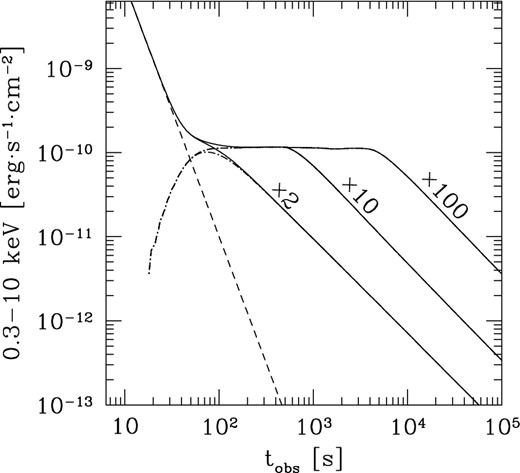
X-ray afterglow light curves from late energy injection into the forward shock. The initial energy in the shock is E0 = 1052 erg and the three light curves correspond (from left to right) to a final energy being, respectively, 2, 10 and 100 times larger. The dashed line represents the continuation of the early steep decay that terminates the prompt emission, while the dash–dotted line shows the forward shock emission only. A redshift z = 1, a uniform external medium of density n = 10 cm−3, and constant microphysics parameters ϵe = 0.1 and ϵB = 0.01 have been assumed.
4 MAKING A PLATEAU AVOIDING AN ENERGY CRISIS
4.1 Forward shock scenario
The standard forward shock scenario can successfully account for the afterglow evolution after about 1 d but fails to reproduce the plateau phase. A backwards extrapolation of the late afterglow flux lies above the plateau, which might therefore be interpreted as the indication that some normally expected radiation is ‘missing’. This can be the case if the radiative efficiency of the forward shock during the early afterglow is smaller than assumed by the simplest version of the standard model. The most obvious way to reduce the efficiency is to relax the assumption that the microphysics parameters stay constant throughout the whole afterglow evolution (Granot et al. 2006; Ioka et al. 2006).
With ϵe ∝ n−1 and from equation (3), a flat plateau extending over two decades in time requires an increase of ϵe by a factor of about 100 from the beginning to the end of the plateau. It is beyond the scope of this paper to decide if this is indeed possible but it is remarkable that acting on one single parameter can lead to the formation of a plateau that also satisfies the observed prompt–afterglow correlations (see Section 5.1).
4.2 Reverse shock scenario
We now suppose that the ejecta emitted by the central engine is made of a ‘head’ with material at high Lorentz factors (Γ ∼ 102–103), followed by a ‘tail’ where the Lorentz factor decreases to much smaller values, possibly close to unity. The head is responsible for the prompt emission while the reverse shock propagating through the tail makes the afterglow.
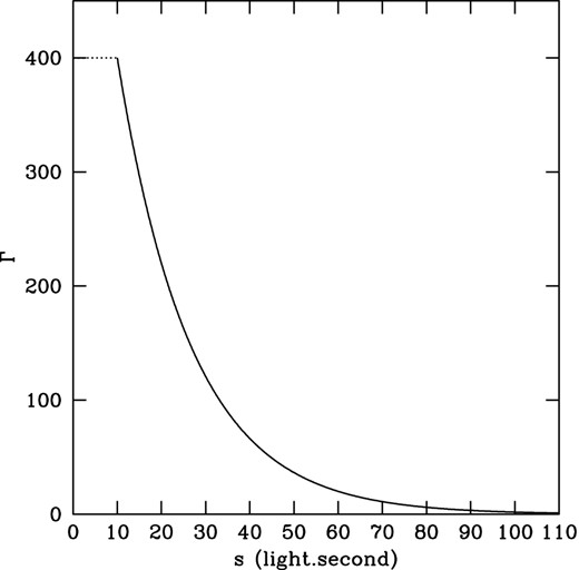
Lorentz factor in the ejecta as a function of the distance from the front (in light.seconds). The ‘head’ (from 0 to 10 light.seconds) is made of material with typical Lorentz factor |$\overline{\Gamma }=400$| while in the tail Γ decreases from 400 to unity following equation (8), so that |${{\rm d}E\over {\rm d}{\rm Log}\,\Gamma }$| is constant.
Using the methods described in Genet et al. (2007) we have obtained the power Pdiss(t) dissipated by the reverse shock as a function of arrival time to the observer for |${\dot{E}}_{\rm H}=10{\dot{E}}_{\rm T}=5\,10^{52}$| erg s−1 (so that equal amounts of energy are injected in the head and tail) and two possibilities for the burst environment: (i) a uniform medium with n = 1000 cm−3 (supposed to be representative of a massive star environment) or (ii) a stellar wind with a wind parameter A* = 1. Going from the dissipated power to actual light curves depends on the assumptions that have to be made for the microphysics parameters. The general shape of the early X-ray afterglow light curves however remains globally similar to the evolution of Pdiss(t) so that some conclusions can already be reached without having to consider the uncertain post-shock microphysics.
Fig. 3 (dotted curves) shows that if energy is evenly distributed in the tail (constant |${\rm{d}E\over \rm{d}{\rm Log}\Gamma }$|) the dissipated power approximately decays as t−1 after about 1000 s, for both a uniform and a wind ambient medium. The contrast κ = Γ/Γbw, where Γ and Γbw are, respectively, the Lorentz factors of the unshocked ejecta and the blast wave, is larger for the uniform medium than for the wind case (κ ≃ 2 and |$\sqrt{2}$|, respectively; see Genet et al. 2007). As seen in Fig. 3 the dissipated power is therefore larger (by a factor of 3-5) in the uniform medium.
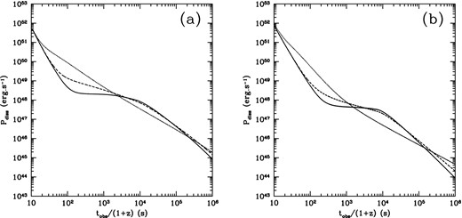
Dissipated power in the reverse shock as a function of observer time for equal amounts of energy EH = ET = 5 1053 erg in the head and tail. The distribution of energy in the tail as a function of Lorentz factor is given by equation (9). (a): uniform external medium of density n = 1000 cm−3, Γ* = 12, q = q ′ = 1.5 (dashed line) and q = q ′ = 2.5 (full line); (b): stellar wind with A* = 1, EH = ET = 5 1053 erg, Γ* = 20, q = q ′ = 3 (dashed line) and q = q ′ = 4.5 (full line). In both panels, the dotted lines have q = q ′ = 0 and correspond to a uniform distribution of energy |${{\rm d}E\over {\rm d}{\rm Log}\Gamma }$| in the tail.
5 BUILDING A SEQUENCE OF MODELS
5.1 Forward shock scenario
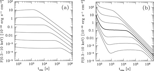
Sequences of X-ray afterglow light curves with plateaus. (a): forward shock scenario with ϵe∝n−1 for n > n0 = 15 cm−3, a wind parameter A* = 0.5 and a gamma-ray efficiency fγ = 0.2. The bottom curve corresponds to an energy injected into the forward shock of 8.5 × 1051 erg and the others to successive multiplication of the energy by a factor F = 2.5; (b): reverse shock scenario with ϵe = 0.1, ϵB = 0.01, an external medium of uniform density n = 1000 cm−3, a distribution of power in the tail given by equation (9) with q = 8/3 and q ′ = 4/3. The thick light curve has EH = ET = 2 1054 erg and Γ* = 16, while the three others above (resp. below) are obtained by successively multiplying (resp. dividing) the energies by F = 2.5 and the Lorentz factors by F1/2. In both panels an index p = 2.2 for the electron spectrum and a redshift z = 1 have been assumed.
5.2 Reverse shock scenario
5.3 Prompt–afterglow correlations
When the sequences obtained in the previous section are transported back into the burst rest frame, the predicted correlations linking the plateau duration tp, luminosity Lp, energy release in X-rays EX and the isotropic gamma-ray energy Eγ,iso can be compared to data. This is done in Fig. 5 for the [Lp, Eγ,iso], [tp, Eγ,iso], [Lp, tp], [Lp/Eγ,iso, tp], [|$E^{\prime }_X, E_{\gamma ,{\rm iso}}$|] and [|$E^{\prime }_X/E_{\gamma ,{\rm iso}},t_{\rm p}$|] relations. Since the plateaus in observed bursts are not all flat contrary to our synthetic ones, we have replaced, for a simple comparison between data and models, the true X-ray energy release by the product |$E^{\prime }_{\rm X}=L_{\rm p}\times t_{\rm p}$|, both for model and data representative points. To account for the likely large dispersion of the |$\Gamma _* \propto E_{\rm iso, 53}^{1/2}$| relation (Hascoët et al. 2014), we also plot sequences corresponding to Γ0 multiplied or divided by 3. Similarly, in the forward shock scenario we represent sequences where the wind parameter A* has been multiplied or divided by 3. In some plots this dispersion has little effect, while in some others, especially [tp, Eγ,iso], it is quite large, but still compatible with the scatter of the data.
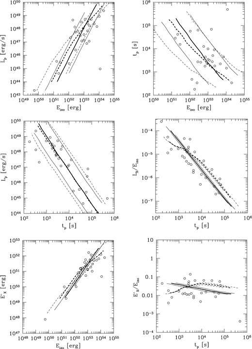
Prompt–afterglow correlations. Open circles show observations; error bars (not shown in this plot) are smaller than the intrinsic scatter of the samples. The thick full line corresponds to the forward shock case and the thick dashed line to the reverse shock case. The thin full and dashed lines, respectively, illustrate the effects of a factor of 3 dispersion in the wind parameter A* and in the relation |$\Gamma _*\propto E_{\gamma ,\rm iso}^{1/2}$| (see the text for details).
6 DISCUSSION AND CONCLUSION
We have addressed in this paper the origin of the plateau phase that is observed in about 50 per cent of the early afterglow light curves observed by Swift XRT (Nousek et al. 2006). We have shown that the commonly invoked cause of plateau formation by continuous energy injection into the forward shock leads to an efficiency crisis for the prompt mechanism as soon as the plateau duration exceeds 103 s.
We have then discussed two alternatives to energy injection, the first one still in the context of the forward shock scenario, the second in the more speculative one where the early afterglow is made by a long-lived reverse shock. Within the forward shock scenario a simple way to produce a plateau is to reduce the radiative efficiency of the shock by acting on the microphysics parameter ϵe. For a wind external medium a simple dependence of the form ϵe ∝ n−1 for n larger than a critical density n0 leads to the formation of a plateau approximately satisfying the prompt–afterglow correlations. The possibility of such a specific behaviour of ϵe remains to be confirmed but it is striking that the temporal evolution of only one parameter in the model can account for both the plateau formation and its phenomenology.
In the reverse shock scenario, the shape of the early afterglow is fixed by the distribution of injected power |${\dot{E}}_{\rm T}(\Gamma )$| in the low Γ tail that is crossed by the shock. Using simple power laws for |${\dot{E}}_{\rm T}(\Gamma )$| we have shown that flat plateaus and correct post-plateau decays can be obtained by adjusting the indices of the power laws. In addition, to satisfy the prompt–afterglow correlations the typical Lorentz factor of the ejecta should increase with burst energy. A relation of the form |$\Gamma \propto E_{\gamma ,{\rm iso}}^{1/2}$|, with a large scatter allowed, provides a reasonable fit of the data. Since the reverse shock is more efficient in a uniform rather than in a wind external medium, the same plateau luminosity can be achieved with three times less energy in the tail and we have then only presented results for this former case. The reverse shock scenario represents a true change of paradigm compared to the standard viewpoint. It has a much larger flexibility in terms of shapes of afterglow light curves. In addition to the capability to produce a plateau it can also account for various accidents such as bumps or steep slopes that are commonly observed (Uhm et al. 2012).
We have limited the present study to the X-ray light curves, and extending the analysis to the optical domain may help to discriminate between the forward and reverse shock scenario we have considered. However, a rich diversity of chromatic behaviours is observed between X-ray and optical domains (e.g. Melandri et al. 2008; Ghisellini et al. 2009; Panaitescu & Vestrand 2011; Li et al. 2012): (a) in a first class of events the optical light curve seems to track the X-ray light curve with similar pre-/post-break decay indices; see for example GRB 050801 (Rykoff et al. 2006), GRB 060729 (Grupe et al. 2007) and GRB 090618 (Cano et al. 2011).2 (b) Then in a second class of events, an optical break is observed in coincidence with the end of the X-ray plateau, but the pre-/post-break decay indices are somewhat different in X-ray and optical (e.g. Panaitescu 2007; Oates et al. 2011). (c) Finally, in a third class of events no clear optical break is seen in coincidence with the end of the X-ray plateau (e.g. GRB 050802; Oates et al. 2007).
Achromatic behaviours (class ‘a’) are most likely the result of a single source (i.e. the forward shock or the reverse shock), where electrons emitting optical and X-rays are in the same radiative regime. This is the case for the two sequences of synthetic GRBs shown in Fig. 4, where both X-rays and optical are produced in fast-cooling regime during the plateau phase.
As for chromatic behaviours, it is not clear whether they are the result of: (i) one single source where X-ray and optical emissions are produced in different radiative regimes. For instance, a situation where optical and X-ray emissions are, respectively, produced in slow-cooling and fast-cooling regimes (if the typical external density and/or ϵB are lower than assumed in the present study), can result in diverse chromatic behaviours. Slow-cooling regime will also make the optical emission much less responsive than X-rays to rapid variations in shock physics (microphysics or dynamics), as it is not dominated by freshly shocked electrons, which can smear out sharp transitions (e.g. breaks) that are well seen in X-rays. This has been investigated in the case of the reverse shock scenario by Uhm & Beloborodov (2007), Genet et al. (2007) and Uhm et al. (2012); (ii) two different sources, respectively, dominating in X-ray and optical domains. In the case where the X-ray plateau is produced by the forward (resp. reverse) shock, invoking the contribution of the reverse (resp. forward) shock will add freedom, which might be necessary in some cases (especially those belonging to class ‘c’). Due to this diverse phenomenology and the different possible interpretations, the extension to optical data would require a detailed modelling case by case, and we do not expect a unique signature of the models in the optical domain. The aim of the present study was first to obtain constraints on models imposed by the X-ray data and especially the prompt–early afterglow correlations.
It is a pleasure to thank Raffaella Margutti who kindly sent us her data on the prompt–afterglow correlations. This work has been financially supported by NSF grant AST-1008334 and the Programme National Hautes Energies (PNHE).
In some cases, achromatic breaks have been proposed to be the result of ‘jet breaks’ (e.g. Sari, Piran & Halpern 1999). This interpretation is however disfavoured for GRB 050801 and GRB 060729, as the measured post-break decay indices (α ≃ −1.5) are typical and much shallower than predicted for a jet break.
