


ABSTRACT
We present the results based on R-band polarimetric follow-up observations of the nearby (∼10 Mpc) Type II-plateau SN 2012aw. Starting from ∼10 d after the supernova (SN) explosion, these polarimetric observations cover ∼90 d (during the plateau phase) and are distributed over nine epochs. To characterize the Milky Way interstellar polarization (ISPMW), we have observed 14 field stars lying in a radius of 10° around the SN. We have also tried to subtract the host galaxy dust polarization component assuming that the dust properties in the host galaxy are similar to that observed for Galactic dust and the general magnetic field follow the large-scale structure of the spiral arms of a galaxy. After correcting the ISPMW, our analysis infer that SN 2012aw has maximum polarization of 0.85 ± 0.08 per cent but polarization angle does not show much variation with a weighted mean value of ∼138°. However, if both ISPMW and host galaxy polarization components are subtracted from the observed polarization values of SN, maximum polarization of the SN becomes 0.68 ± 0.08 per cent. The distribution of Q and U parameters appears to follow a loop-like structure. The evolution of polarimetric light curve properties of this event is also compared with other well-studied core-collapse SNe of similar type.
1 INTRODUCTION
Core-collapse supernovae (CCSNe) exhibit significant level of polarization during various phases of their evolution at optical/infrared wavelengths. In general, the degree of polarization of different types of SNe seems to increase with decreasing mass of the stellar envelope at the time of explosion (see Wheeler 2000; Leonard et al. 2001; Wang et al. 2001; Leonard & Filippenko 2005). Type II SNe are polarized at level of ∼1–1.5 per cent. However, Type Ib/c SNe (also known as stripped-envelope SNe, as the outer envelopes of hydrogen and/or helium of their progenitors are partially or completely removed before the explosion) demonstrate significantly higher polarization in comparison to Type II SNe (for more details, see Leonard & Filippenko 2001; Kawabata et al. 2002, 2003; Wang et al. 2003a; Gorosabel et al. 2006; Maund et al. 2007, 2013; Patat et al. 2012; Tanaka et al. 2012, and references therein). The higher polarization values observed in case of Type Ib/c SNe most probably arise due to extreme departure from the spherical symmetry (Chugai 1992; Höflich, Khokhlov & Wang 2001; Khokhlov & Höflich 2001).
Theoretical modelling predicts that in general CCSNe show the degree of asymmetry of the order of 10–30 per cent if modelled in terms of oblate/prolate spheroids (e.g. Hoflich 1991). Numerical simulations (see Kasen, Thomas & Nugent 2006; Dessart & Hillier 2011) indicate that in case of Type II SNe, the level of polarization is also influenced by SN structure (e.g. density and ionization), apart from their initial mass and rotation. The possible progenitors of Type IIP SNe are low-mass red/blue supergiants and their polarization studies are extremely useful to understand the SN structure in detail. In spite of being the most common subtypes among the known CCSNe, polarization studies of Type IIP SNe have been done only in a handful of cases (e.g. Barrett 1988; Leonard et al. 2001, 2006, 2012a; Leonard & Filippenko 2001; Chugai 2006; Chornock et al. 2010). In general, intrinsic polarization in these SNe are observed below 1 per cent but few exceptions exist in literature (for example Chornock et al. 2010 reported ∼1.5 per cent for SN 2006ov).
Systematic polarimetric studies have been started, only after the observations of Type IIP SN 1987A (see Cropper et al. 1988; Mendez et al. 1988; Jeffery 1991). Shapiro & Sutherland (1982) first pointed out that polarimetry provides direct powerful probe to understand the SN geometry (see also McCall 1984; Hoflich 1991). Polarization is believed to be produced due to electron scattering within the SN ejecta. When light passes through the expanding ejecta of CCSNe, it retains information about the orientation of layers. In spherically symmetric scenario, the equally present directional components of the electric vectors will be cancelled out to produce zero net polarization. If the source is aspherical, incomplete cancellation occurs which finally imprints a net polarization (see fig. 1 of Filippenko & Leonard 2004 and Leonard & Filippenko 2005). In addition to asphericity of the electron scattering atmosphere, there are several other processes which can produce polarization in CCSNe such as scattering by dust (e.g. Wang & Wheeler 1996), clumpy ejecta or asymmetrically distributed radioactive material within the SN envelope (e.g. Hoeflich 1995; Chugai 2006), and aspherical ionization produced by hard X-rays from the interaction between the SN shock front and a non-spherical progenitor wind (Wheeler & Filippenko 1996).
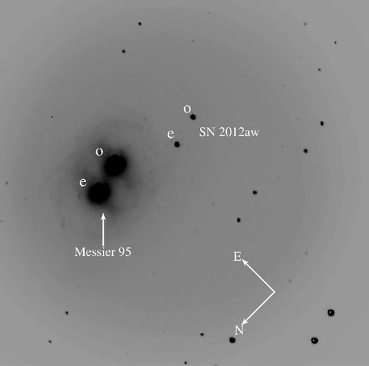
The R-band image of the SN 2012aw field around the host galaxy M95, observed on 2012 April 17 using AIMPOL with the 1.04 m ST, India. Each object has two images. The ordinary and extraordinary images of SN 2012aw and host galaxy are labelled as o and e, respectively. The galaxy is marked with a white arrow and the SN is located 60 arcsec west, 115 arcsec south of the centre of M95 galaxy. North and east directions are also indicated.
To diagnose the underlying polarization in SNe explosions, two basic techniques, i.e. broad-band polarimetry and spectropolarimetry have been used. Both of these techniques have advantages and disadvantages relative to each other. One of the main advantages of spectropolarimetry of SNe with respect to broad-band polarimetry is its ability to infer geometric and dynamical information for the different chemical constituents of the explosion. Broad-band polarimetric observations construct a rather rough picture of the stellar death but require lesser number of total photons than spectropolarimetry. Hence, broad-band polarimetric observations can be extended to objects at higher redshifts or/and they allow to enhance the polarimetric coverage and sampling of the light curve (LC), especially at epochs far from the maximum when the SN is dimmer.
The scope of this paper uses imaging polarimetric observations in the R band using a metre class telescope when the SN 2012aw was bright enough (R < 13.20 mag).
1.1 SN 2012aw
SN 2012aw was discovered in a face-on (i ∼ 54| $_{.}^{\circ}$|6, from HyperLEDA1), barred and ringed spiral galaxy M95 (NGC 3351) by P. Fagotti on CCD images taken on 2012 March 16.85 ut with a 0.5-m reflector (cf. CBET 3054, Fagotti et al. 2012). The SN was located 60 arcsec west and 115 arcsec north of the centre of the host galaxy with coordinates |$\alpha = 10^{\rm h} 43^{\rm m} 53_{.}^{\mathrm{s}}73$|, δ = +11°40′17| $_{.}^{\prime\prime}$|9 (equinox 2000.0). This SN discovery was also confirmed independently by A. Dimai on 2012 March 16.84 ut, and J. Skvarc on March 17.90 ut (more information available in Fagotti et al. 2012, CBET 3054; see also special notice no. 269 available at AAVSO2). The spectra obtained on March 17.77 ut by Munari, Vagnozzi & Castellani (2012) with the Asiago Observatory 1.22-m reflector showed a very blue continuum, essentially featureless, with no absorption bands and no detectable emission lines. In subsequent spectra taken on March 19.85 ut (Itoh, Ui & Yamanaka 2012) and 19.92 ut (Siviero et al. 2012), the line characteristics finally led to classify it as a young Type IIP supernova. The explosion date of this event is precisely determined by Fraser et al. (2012) and Bose et al. (2013). We adopt 2012 March 16.1 ± 0.8 d (JD 245 6002.6 ± 0.8, taken from the later study) as time of explosion throughout this article. At a distance of about 10 Mpc (cf. Freedman et al. 2001; Russell 2002; Bose et al. 2013), this event provided us a good opportunity to study its detail polarimetric properties.
The progenitor of this SN has been detected both in ground and space based pre-explosion images and its distinct characteristics are analysed. In pre-SN explosion images obtained with HST3 + WFPC2,4 VLT5 + ISAAC6 and NTT7+SOFI,8 Fraser et al. (2012) found that the progenitor is a red supergiant (mass 14–26 Mȯ). An independent study by Van Dyk et al. (2012b) confirmed these findings (mass 15–20 Mȯ). However, Kochanek, Khan & Dai (2012) have a different view and have concluded that progenitor mass in earlier studies are significantly overestimated and that the progenitor's mass is <15 Mȯ. Immediately after the discovery, several groups have started the follow-up observations of this event in different wavelengths (see, e.g. Immler & Brown 2012; Stockdale et al. 2012; Bayless et al. 2013; Munari et al. 2013; Yadav et al. 2014). Early epoch (4–270 d) low-resolution optical spectroscopic and dense photometric follow-up (in UBVRI/griz bands) observations of SN 2012aw have been analysed by Bose et al. (2013). In a recent study, Jerkstrand et al. (2014) have presented nebular phase (between 250 and 451 d) optical and near-infrared spectra of this event and have analysed it with spectral model calculations. Furthermore, the preliminary analysis of optical spectropolarimetric data of SN 2012aw, revealed that outer ejecta are substantially asymmetric (Leonard et al. 2012b).
In this paper, we present Cousins R-band polarimetric follow-up observations of SN 2012aw. The observations and data reduction procedures are presented in Section 2. Estimation of intrinsic polarization is described in Section 3. Finally, results and conclusions are presented in Sections 4 and 5, respectively.
2 OBSERVATIONS AND DATA REDUCTION
Polarimetric observations of SN 2012aw field were carried out during nine nights, i.e. March 26, 28, 29; April 16, 17; May 15, 19, 21 and 2012 June 12 using the ARIES Imaging Polarimeter (AIMPOL; Rautela, Joshi & Pandey 2004) mounted at the Cassegrain focus of the 1.04 m Sampurnanand telescope (ST) at Manora Peak, Nainital. This telescope is operated by the Aryabhatta Research Institute of Observational sciences (ARIES), India. Complete log of these observations is presented in Table 1. The position of SN, which is fairly isolated from the host galaxy and lies on a smooth and faint galaxy background is shown in Fig. 1. The observations were carried out in R (|$\lambda _{R_{\rm eff}}$| = 0.67 μm) photometric band using liquid nitrogen cooled Tektronix 1024 × 1024 pixel2 CCD camera. Each pixel of the CCD corresponds to 1.73 arcsec and the field of view (FOV) is ∼8 arcmin in diameter on the sky. The full width at half-maximum of the stellar images vary from 2 to 3 pixels. The readout noise and the gain of the CCD are 7.0 e− and 11.98 e−/ADU, respectively.
Polarimetric observation log and estimated polarimetric parameters of SN 2012aw.
| ut Date | JD | Phasea | Observed | Intrinsic (ISPMW subtracted) | Intrinsic (ISPMW + ISPHG subtracted) | |||||||||||||||
|---|---|---|---|---|---|---|---|---|---|---|---|---|---|---|---|---|---|---|---|---|
| (2012) | (245 0000) | (d) | |$P_{R} \pm \sigma _{P_{R}}$| | |$\theta {_R} \pm \sigma _{\theta {_R}}$| | |$P_{R} \pm \sigma _{P_{R}}$| | |$\theta {_R} \pm \sigma _{\theta {_R}}$| | |$P_{R} \pm \sigma _{P_{R}}$| | |$\theta {_R} \pm \sigma _{\theta {_R}}$| | ||||||||||||
| (per cent) | (°) | (per cent) | (°) | (per cent) | (°) | |||||||||||||||
| Mar 26 | 6013.35 | 10.75 | 0.58 ± 0.46 | 131.4 ± 22.9 | 0.61 ± 0.46 | 138.9 ± 21.6 | 0.39 ± 0.46 | 134.2 ± 33.4 | ||||||||||||
| Mar 28 | 6015.23 | 12.63 | 0.56 ± 0.03 | 132.0 ± 1.5 | 0.60 ± 0.03 | 139.6 ± 1.4 | 0.38 ± 0.03 | 135.1 ± 2.2 | ||||||||||||
| Mar 29 | 6016.28 | 13.68 | 0.49 ± 0.08 | 132.2 ± 4.6 | 0.53 ± 0.08 | 140.8 ± 4.3 | 0.31 ± 0.08 | 136.1 ± 7.3 | ||||||||||||
| Apr 16 | 6034.18 | 31.58 | 0.24 ± 0.17 | 132.0 ± 21.0 | 0.30 ± 0.17 | 147.8 ± 16.7 | 0.07 ± 0.17 | 150.5 ± 72.8 | ||||||||||||
| Apr 17 | 6035.25 | 32.65 | 0.26 ± 0.01 | 142.6 ± 1.0 | 0.36 ± 0.01 | 154.0 ± 0.8 | 0.15 ± 0.01 | 164.8 ± 1.8 | ||||||||||||
| May 15 | 6063.05 | 60.45 | 0.87 ± 0.08 | 123.8 ± 2.6 | 0.85 ± 0.08 | 129.0 ± 2.6 | 0.68 ± 0.08 | 123.3 ± 3.3 | ||||||||||||
| May 19 | 6067.04 | 64.44 | 0.54 ± 0.01 | 124.3 ± 0.5 | 0.54 ± 0.01 | 132.7 ± 0.5 | 0.35 ± 0.01 | 123.6 ± 0.8 | ||||||||||||
| May 21 | 6069.08 | 66.48 | 0.43 ± 0.06 | 112.3 ± 4.0 | 0.37 ± 0.06 | 122.7 ± 4.6 | 0.28 ± 0.06 | 103.4 ± 6.2 | ||||||||||||
| Jun 14 | 6093.23 | 90.63 | 0.47 ± 0.14 | 128.2 ± 8.5 | 0.49 ± 0.14 | 137.5 ± 8.2 | 0.29 ± 0.14 | 129.9 ± 14.1 | ||||||||||||
awith reference to the explosion epoch JD 245 6002.6.
Observational detail of 14 isolated field stars selected to subtract the interstellar polarization. Observations of all field stars were performed on 2013 January 20 in the R band with the 1.04 m ST. All these stars were selected with known distances and within 10° radius around SN 2012aw. The distance mentioned in the last column has been taken from van Leeuwen (2007) catalogue.
| Star | RA (J2000) | Dec. (J2000) | |$P_{R} \pm \sigma _{P_{R}}$| | |$\theta {_R} \pm \sigma _{\theta {_R}}$| | Distance |
|---|---|---|---|---|---|
| id | (°) | (°) | (per cent) | (°) | (in pc) |
| HD 99028a | 170.98071 | +10.52960 | 0.08 ± 0.00 | 167.9 ± 1.7 | 23.7 ± 0.5 |
| HD 88830a | 153.73935 | +09.21180 | 0.10 ± 0.01 | 116.8 ± 1.8 | 36.3 ± 3.8 |
| HD 87739a | 151.78235 | +08.76970 | 0.05 ± 0.01 | 99.9 ± 6.6 | 85.0 ± 8.3 |
| HD 97907a | 168.96624 | +13.30750 | 0.17 ± 0.05 | 59.6 ± 9.5 | 99.6 ± 12.1 |
| HD 88282a | 152.72730 | +07.69460 | 0.12 ± 0.01 | 79.1 ± 1.8 | 118.5 ± 10.0 |
| HD 87635a | 151.57707 | +07.94470 | 0.17 ± 0.00 | 89.0 ± 0.5 | 135.7 ± 19.9 |
| HD 87915a | 152.08824 | +07.57300 | 0.11 ± 0.01 | 86.4 ± 1.6 | 193.1 ± 34.7 |
| HD 87996a | 152.20123 | +06.71740 | 0.20 ± 0.04 | 62.5 ± 5.6 | 243.3 ± 91.2 |
| HD 88514a | 153.15102 | +07.67730 | 0.18 ± 0.03 | 90.5 ± 4.5 | 254.5 ± 82.9 |
| G 452 | 160.45186 | +12.10886 | 0.10 ± 0.01 | 22.6 ± 2.4 | 261.1 ± 70.9 |
| BD+12 2250 | 161.08996 | +11.33560 | 0.12 ± 0.08 | 100.1 ± 18.0 | 286.5 ± 91.1 |
| BD+13 2299 | 161.41026 | +12.46724 | 0.20 ± 0.00 | 72.4 ± 0.8 | 314.5 ± 87.0 |
| HD 93329 | 161.65268 | +11.18412 | 0.12 ± 0.03 | 144.8 ± 5.8 | 358.4 ± 118.2 |
| HD 92457 | 160.15550 | +12.07868 | 0.05 ± 0.07 | 27.8 ± 41.3 | 460.8 ± 191.1 |
aStars with available V-band polarimetry from Heiles (2000) catalogue.
BD+12 2250, BD+13 229, G 452, HD 93329 and HD 92457 are the stars within 2° radius field around the SN.
The AIMPOL consists of a half-wave plate modulator and a Wollaston prism beam-splitter. In order to obtain the measurements with good signal-to-noise ratio, images that were acquired at each position of half-wave plate were combined. Since AIMPOL is not equipped with a narrow-window mask, care was taken to exclude the stars that have contamination from the overlap of ordinary and extraordinary images of one star on the same of another star in the FOV.
To correct the measurements for the instrumental polarization and the zero-point PA, we observed a number of unpolarized and polarized standards, respectively, taken from Schmidt, Elston & Lupie (1992). Measurements for the standard stars are compared with those taken from the Schmidt et al. (1992). The observed values of degree of polarization [P (per cent)] and position angle [θ(°)] were in good agreement (within the observational errors) with those published in Schmidt et al. (1992). The instrumental polarization of AIMPOL on the 1.04 m ST has been characterized and monitored since 2004 for different projects and found to be ∼0.1 per cent in different bands (e.g. Rautela et al. 2004; Pandey et al. 2009; Eswaraiah et al. 2011, 2012, 2013, and references therein).
3 ESTIMATION OF INTRINSIC POLARIZATION
The observed polarization measurements of a distant SN could be composed of various components such as interstellar polarization due to Milky Way dust (ISPMW), interstellar polarization due to host galactic dust (ISPHG) and due to instrumental polarization. As described in the previous section, we have already subtracted the instrumental polarization. Therefore, now it is essential to estimate the contributions due to ISPMW and ISPHG, and to remove them from the total observed polarization measurements of SN. However, there is no totally reliable method to derive the ISPMW/ISPHG of SN polarimetry observationally and utmost careful analysis is required to avoid any possible fictitious result. In the following sections, we discuss in detail about the ISPMW and ISPHG estimation in the present set of observations.
3.1 Interstellar polarization due to Milky Way (ISPMW)
To estimate the interstellar polarization in the direction of SN 2012aw, we have performed R-band polarimetric observations of 14 isolated and non-variable field stars (which do not show either emission features or variability flag in the SIMBAD data base) distributed in a region of 10° radius around SN. Table 2 lists the observational detail of these stars. All 14 stars have distance information from Hipparcos parallax (van Leeuwen 2007) and out of these, nine stars have both polarization (Heiles 2000) and distance measurements. In Fig. 2 (left-hand panels), we show the distribution of degree of polarization and PAs for these nine stars. The weighted mean values of PV and θV of eight out of these nine stars (after excluding one star whose PV is 0.007 per cent) are found to be 0.071 ± 0.010 per cent and 83° ± 4°, respectively. Because our polarimetric observations are performed in the R band therefore, to correct for ISPMW component and to study the intrinsic behaviour of SN, we have used polarization measurements of 14 field stars observed on 2013 January 20 in the R band (see Table 2). The distribution of PR and θR values of these stars is shown in right-hand panels of Fig. 2. All the observed 14 stars are shown with filled circles. As revealed by both left-hand and upper-right panels of Fig. 2, the amount of degree of polarization shows an increasing trend with distance. It is worthwhile to note that, in the upper-right panel, the degree of polarization (PR) seems to show a sudden jump from ∼0.1 per cent at the distance of ∼100 pc to ∼0.2 per cent at a distance of ∼250 pc, thereby indicating the presence of a dust layer (shown with a grey region in Fig. 2) at ∼100 pc. Whereas, the PAs of the stars from Heiles catalogue (left bottom panel) and those observed from the present set-up in the R band (except few stars) are distributed between 50° and 100° as shown with the dashed lines (in Fig. 2). The Gaussian mean value of θR using 14 stars is found to be ∼82°. This indicates the presence of a uniform dust layer towards the direction of SN 2012aw, which nearly contributes ∼0.1-0.2 per cent of polarization and having a mean magnetic field orientation ∼82°. Therefore, we believe that most probably, the ISPMW component has been dominated by the contribution from this dust layer.
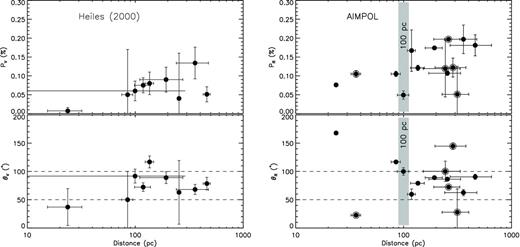
Distribution of polarization and PA of stars around SN 2012aw. Left-hand panel: nine isolated field stars with known polarization and parallax measurements from Heiles (2000) and van Leeuwen (2007), respectively. Right-hand panel: same as left-hand panel but for 14 isolated stars with R-band polarimetric data using AIMPOL and with distance from van Leeuwen (2007) catalogue. Filled circles denote nine common stars in both left- and right-hand panels. The encircled filled circles are five stars distributed within a 2° radius around the location of SN 2012aw. The grey region represents the possible presence of a dust layer around 100 pc distance.
Estimated polarimetric parameters for ISPMW (see Section 3.1 for detail).
| Number | Distance | |$\langle Q_{R} \pm \sigma _{Q_{R}}\rangle$| | |$\langle U_{R} \pm \sigma _{U_{R}}\rangle$| | |$\langle P_{R} \pm \sigma _{P_{R}}\rangle$| | |$\langle \theta {_R} \pm \sigma _{\theta {_R}}\rangle$| |
|---|---|---|---|---|---|
| of stars | (pc) | (per cent) | (per cent) | (per cent) | (°) |
| 14a | all distances | −0.101 ± 0.002 | 0.012 ± 0.002 | 0.102 ± 0.002 | 86.49 ± 0.54 |
| 10 | >100 | −0.154 ± 0.002 | 0.032 ± 0.002 | 0.157 ± 0.002 | 84.10 ± 0.43 |
aAll stars within 10° radius around the SN.
The reddening, E(B − V) due to Milky Way dust in the direction of SN 2012aw, as derived from the 100-μm all-sky dust extinction map of Schlegel, Finkbeiner & Davis (1998), was found to be 0.0278 ± 0.0002 mag. According to the mean polarization efficiency relation Pmean = 5 × E(B − V) (Serkowski, Mathewson & Ford 1975), the polarization value is estimated to be Pmean ∼ 0.14 per cent which closely matches with the weighted mean polarization value, 0.157 ± 0.002 per cent obtained using the 10 fields stars distributed beyond 100 pc distance (cf. Table 3). It is clear that polarization values obtained both from the present observations of the field stars and mean polarization efficiency relation are similar which implies that the dust grains in the local interstellar medium exhibit mean polarization efficiency.
3.2 Interstellar polarization due to host galactic dust (ISPHG)
The reddening, E(B − V), due to dust in the SN 2012aw host galaxy was found to be 0.046 ± 0.008 mag (see Bose et al. 2013). This value was derived using the empirical correlation, between reddening and Na i D lines, given by Poznanski, Prochaska & Bloom (2012). As described in Section 3.1, the weighted mean value of polarization of 10 field stars situated beyond 100 pc distance (0.157 ± 0.002 per cent) and the extinction (0.0278 ± 0.0002 mag) due to the Galactic dust in the line of sight to the SN suggest that Galactic dust exhibits a mean polarization efficiency. To subtract the ISPHG component, we should estimate the degree of polarization and the magnetic field orientation of the host galaxy at the location of the SN.
The properties of dust grains in the nearby galaxies have been investigated in detail only in a handful of cases and diverse nature of dust grains have been established in these studies. In case of SN 1986G, Hough et al. (1987) probed the ISPHG component due to the dust lanes in the host galaxy NGC 5128 (Centaurus A) and validated that the size of the dust grains is smaller than typical Galactic dust grains. In another study (SN 2001el), the grain sizes were found to be smaller for NGC 1448 (Wang et al. 2003a). However, in some cases, polarization efficiency of dust has been estimated to be much higher than the typical Galactic dust (see e.g. Leonard et al. 2002; Clayton et al. 2004). For the present study, we assume that the dust grain properties of the M95 are similar to that the Galactic dust, and follow mean polarization efficiency relation (i.e. Pmean = 5 × E(B − V); Serkowski et al. 1975). Therefore, the estimated polarization value would be ∼0.23 per cent.
Another required parameter is the orientation of the magnetic field near the location of the SN. It is well known that large-scale Galactic magnetic field runs almost parallel (i.e. perpendicular to the line connecting a point with the galaxy centre) to the spiral arms (Scarrott, Rolph & Semple 1990; Scarrott et al. 1991; Heiles 1996; Han 2009). Interestingly, as shown in Fig. 1, the SN 2012aw is located nearer to one of the spiral arms of the host galaxy. On the basis of the structure of the spiral arm and the location of SN, we have estimated the tangent to the spiral arm at the location of the SN (see Fig. 3), which makes approximately 147° from the equatorial north increasing towards the east. We assume, on the basis of structure of the spiral arms and the magnetic field orientation that the magnetic field orientation in the host galaxy at the location of the SN is to be ∼147°. Here, we would like to emphasize that present procedure of considering magnetic field for the host of SN 2012aw is well established in previous spectropolarimetric studies of Type IIP SN 1999em (Leonard et al. 2001) and Type IIb SN 2001ig (Maund et al. 2007).
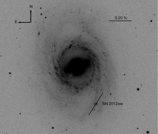
SDSSg-band image (7.7 arcmin × 7.2 arcmin) of the SN field containing the galaxy M95. A vector with a degree of polarization 0.23 per cent and position angle of 147° is drawn at the location of SN 2012aw (see text in Section 3.2 for details). A vector with a 0.20 per cent polarization and PA of 90° is shown for a reference (top right). The approximate orientation of the magnetic field at the location of SN has been determined on the basis of structure of the spiral arm (see Section 3.2 for more details). The location of the SN is represented by a square symbol. North is up and east is to left as shown in the figure.
As shown in Fig. 3, a black vector with a length of 0.23 per cent and orientation of 147° is drawn at the location of the SN which is shown with a square symbol. Hence, by assuming that the amount of polarization and the PA due to the host galaxy are as 0.23 per cent and 147°, the Stokes parameters are estimated to be |$Q_{\it {\rm ISP}_{\it {\rm HG}}}$| = 0.11 per cent, |$U_{\it {\rm ISP}_{\it {\rm HG}}}$| = −0.25 per cent. To get the intrinsic Stokes parameters and hence the amount of polarization and PAs purely due to the SN 2012aw, these values were subtracted vectorially from the ISPMW corrected Stokes parameters as described in Section 3.1. The intrinsic (ISPMW + ISPHG subtracted) polarization and PAs of SN are listed in the columns 8 and 9 of Table 1 and plotted in Fig. 4(a) and (b), respectively, with open circles connected with broken lines.
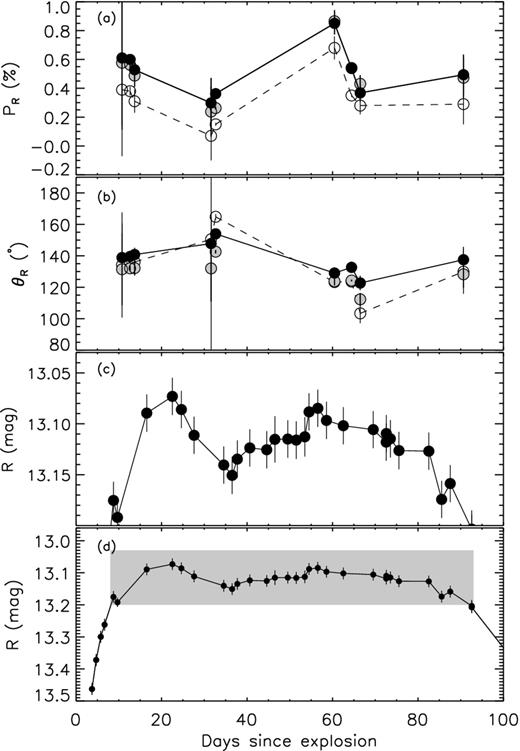
Panels (a) and (b): temporal evolution of polarization and PAs of SN 2012aw in the R band, respectively. Filled circles connected with thick lines denote the temporal evolution of polarization and PAs after subtracting the ISPMW component only, whereas those corrected for both ISPMW + ISPHG components were represented with open circles connected with broken lines. The observed polarization parameters are shown with grey filled circles in panels (a) and (b). The bottom panel (d) shows the calibrated R-band LC of SN 2012aw obtained with ST (see Bose et al. 2013). The photometric data shown with shaded region in the bottom panel (d) is replotted in panel (c) for a better clarity.
4 DISCUSSION
4.1 Polarization light curve (PLC) analysis
In this section, we analyse the evolution of the PLC and its possible resemblance with the photometric LC of the SN 2012aw as shown in Fig 4. The calibrated R-band magnitudes have been taken from Bose et al. (2013), which show different evolutionary phases of the LC as described in Grassberg, Imshennik & Nadyozhin (1971), Falk & Arnett (1977), Utrobin (2007). Since in the present study, polarimetric data sets are limited up to the plateau phase, in Fig. 4 (panels c and d), only the adiabatic cooling phase and the phase of cooling and recombination wave are shown.
The temporal variation of ISPMW corrected degree of polarization (PR) values (shown with filled circles, Fig. 4a) shows a maximum and minimum values of ∼0.9 and 0.3 per cent, respectively, with a possible trend of variations in accordance with the R-band LC as shown in panel 4(c). Although there is a significant reduction in ISPMW + ISPHG corrected PR values (open circles, Fig. 4a), its resemblance with photometric LC (panel c) remain similar. However, both ISPMW and ISPMW + ISPHG corrected PAs (θR, shown with filled circles in Fig. 4b) do not show much variation during the similar epochs of observations and are distributed around a weighted mean value of ∼138°. Interestingly, first (10–14 d) three measurements of ISPMW corrected PR and θR are almost constant. During this adiabatic cooling phase, the SN LC seems to be brightened by ∼0.12 mag as shown in Fig. 4(c).
It is worthwhile to note that dips observed around 35 d in the LC of the SN and in the ISPMW + ISPHG corrected PR are temporally correlated with a minimum amount of polarization (∼0.07 per cent). This observed feature during the end of the adiabatic cooling or early recombination phase could be attributed to several reasons e.g. (i) changes in the geometry, i.e. transition from more asphericity to sphericity of SN, (ii) modification in density of scatterers (electrons and/or ions), (iii) mechanism of scattering, i.e. single and (or) multiple scattering, (iv) changes in the clumpiness in the SN envelope, (v) changes in the electron-scattering atmosphere of SN and (vi) interaction of SN with a dense circumstellar medium. In the recombination phase (∼40 d onwards), the evolution in the values of ISPMW + ISPHG corrected PR and θR are in such a way that the amount of polarization shows an increasing trend. This increasing trend could suggest that during the recombination phase and onwards, the geometry of the SN envelope could have acquired more asphericity.
If we assume that the ISPMW and ISPHG components are constant, then the changes observed in the temporal variation of intrinsic polarization measurements of the SN could purely be attributed to variations in the geometry of the SN along with the other possible reasons such as the interaction of the SN shock with the ambient medium. However, these properties could be well addressed using high-resolution spectroscopic/spectropolarimetric investigations which are beyond the scope of this paper.
4.2 Q and U parameters
The Q − U parameters, representing different projections of the polarization vectors, are used as a powerful tool to examine the simultaneous behaviour of the polarization and the PA with wavelengths (see e.g. Wang et al. 2003a,b). The pattern of the variation in Q − U plane does not depend upon the ISPMW/ISPHG corrections. However, the ISPMW/ISPHG subtracted parameters are dependent on the corrections applied to the observed values. A small change in ISPMW/ISPHG may considerably affect the PA values.
The estimated Q − U parameters (observed and intrinsic) for SN 2012aw are presented in Table 4 and are plotted in Fig. 5. The left and middle panels of this figure show the observed and ISPMW subtracted parameters and, the right-hand panel represents intrinsic parameters after subtracting both ISPMW + ISPHG contribution as discussed in Section 3. The square symbol connected with large circles drawn nearer to the solar neighbourhood in the middle and right panels, respectively, indicate ISPMW (|$Q_{\it {\rm ISP}_{\it {\rm MW}}}$| = −0.154, |$U_{\it {\rm ISP}_{\it {\rm MW}}}$| = 0.032) and ISPMW + ISPHG (|$Q_{\it {\rm ISP}_{\it {\rm MW}} + {\rm ISP}_{\it {\rm HG}}}$| = −0.060, |$U_{\it {\rm ISP}_{\it {\rm MW}} + {\rm ISP}_{\it {\rm HG}}}$| = −0.178) components.
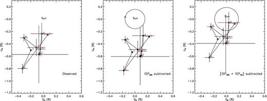
Stokes Q and U parameters of SN 2012aw. Left-hand panel: grey filled circles are the observed parameters. Middle panel: the data have been corrected for the ISPMW component only (black filled circle; see text). Right-hand panel: after correcting both ISPMW + ISPHG components (open circle; see text). The square symbol connected with large circles drawn nearer to the solar neighbourhood in the middle and right panels, respectively, indicate the ISPMW and ISPMW + ISPHG components. Numbers labelled with 1–9 (red colour) and connected with continuous lines, indicate the temporal order.
Observed and intrinsic (ISPMW and ISPMW + ISPHG subtracted) Q-U parameters for SN 2012aw.
| ut Date | JD | Phasea | Observed | Intrinsic (ISPMW subtracted) | Intrinsic (ISPMW + ISPHG subtracted) | |||||||||||||||
|---|---|---|---|---|---|---|---|---|---|---|---|---|---|---|---|---|---|---|---|---|
| (2012) | 245 0000 | (d) | |$Q_{R} \pm \sigma _{Q_{R}}$| | |$U{_R} \pm \sigma _{U{_R}}$| | |$Q_{R} \pm \sigma _{Q_{R}}$| | |$U{_R} \pm \sigma _{U{_R}}$| | |$Q_{R} \pm \sigma _{Q_{R}}$| | |$U_{R} \pm \sigma _{U_{R}}$| | ||||||||||||
| (per cent) | (per cent) | (per cent) | (per cent) | (per cent) | (per cent) | |||||||||||||||
| Mar 26 | 6013.35 | 10.75 | −0.072 ± 0.461 | −0.573 ± 0.464 | 0.082 ± 0.461 | −0.605 ± 0.464 | −0.012 ± 0.461 | −0.394 ± 0.464 | ||||||||||||
| Mar 28 | 6015.23 | 12.63 | −0.058 ± 0.029 | −0.560 ± 0.029 | 0.095 ± 0.029 | −0.592 ± 0.029 | 0.002 ± 0.029 | −0.382 ± 0.029 | ||||||||||||
| Mar 29 | 6016.28 | 13.68 | −0.048 ± 0.079 | −0.486 ± 0.078 | 0.106 ± 0.079 | −0.518 ± 0.078 | 0.012 ± 0.079 | −0.308 ± 0.078 | ||||||||||||
| Apr 16 | 6034.18 | 31.58 | −0.025 ± 0.174 | −0.237 ± 0.173 | 0.129 ± 0.174 | −0.269 ± 0.173 | 0.035 ± 0.174 | −0.059 ± 0.173 | ||||||||||||
| Apr 17 | 6035.25 | 32.65 | 0.069 ± 0.010 | −0.254 ± 0.009 | 0.223 ± 0.010 | −0.286 ± 0.009 | 0.129 ± 0.010 | −0.076 ± 0.009 | ||||||||||||
| May 15 | 6063.05 | 60.45 | −0.330 ± 0.077 | −0.800 ± 0.077 | −0.176 ± 0.077 | −0.832 ± 0.077 | −0.269 ± 0.077 | −0.622 ± 0.077 | ||||||||||||
| May 19 | 6067.04 | 64.44 | −0.198 ± 0.009 | −0.504 ± 0.009 | −0.044 ± 0.010 | −0.536 ± 0.009 | −0.137 ± 0.010 | −0.326 ± 0.009 | ||||||||||||
| May 21 | 6069.08 | 66.48 | −0.307 ± 0.059 | −0.303 ± 0.059 | −0.153 ± 0.059 | −0.335 ± 0.059 | −0.247 ± 0.059 | −0.125 ± 0.059 | ||||||||||||
| Jun 14 | 6093.23 | 90.63 | −0.111 ± 0.141 | −0.460 ± 0.140 | 0.043 ± 0.141 | −0.492 ± 0.140 | −0.050 ± 0.141 | −0.282 ± 0.140 | ||||||||||||
awith reference to the explosion epoch JD 245 6002.6
Since, in the present case, the data points are limited, a firm conclusion could not be robustly drawn on behalf of Q and U parameters. However, it seems that in all three panels of Fig. 5, these data points show scattered distribution, which seems to form a loop-like structure on Q − U plane. This kind of structure has been also observed in case of SN 1987A (Cropper et al. 1988), SN 2004dj (Leonard et al. 2006) and SN 2005af (Pereyra et al. 2006). Although, it is to be noted that if we ignore one of the data points (observed on May 21), the variation of Q − U parameters will more likely to follow straight line and in this case the previous interpretation may not be true.
4.3 Comparison with other Type IIP events
We have collected polarization parameters of a few well-observed Type IIP SNe from the literature: SN 2008bk (Leonard et al. 2012a), SN 2007aa and SN 2006ov (Chornock et al. 2010), 2005af (Pereyra et al. 2006), 2004dj (Leonard et al. 2006), 1999em (Leonard et al. 2001) and SN 1987A (Barrett 1988) for which polarimetric observations have been performed for two or more epochs. Except for SN 1987A, SN 2005af and SN 2012aw, the data for other events are spectropolarimetric only. The intrinsic polarization values of SN 2012aw along with other SNe are plotted in Fig. 6. It is worthwhile to note that the explosion epochs of SN 1987A (see Bionta et al. 1987; Hirata et al. 1987), SN 1999em (see Elmhamdi et al. 2003) and SN 2012aw are known precisely, but there is uncertainty in the estimation of explosion epoch for other events (SN 2004dj, SN 2005af, SN 2006ov, SN 2007aa and SN 2008bk). In case of SN 2004dj, Leonard et al. (2006) considered the explosion epoch on JD 245 3200.5 but Zhang et al. (2006) estimated it on JD 245 3167 ± 21. With an uncertainty of few weeks, the explosion epoch for SN 2005af is estimated to be on JD 245 3379.5 (see Kotak et al. 2006). For SN 2006ov, Blondin et al. (2006) estimated the expected date of explosion ∼36 d before the discovery (Nakano, Itagaki & Kadota 2006) but Li et al. (2007) reasonably constraints its explosion about three months before the discovery. We follow the later study in the present analysis. Similarly, we considered explosion epoch for SN 2007aa, ∼20 d before the discovery (see Doi et al. 2007; Folatelli, Gonzalez & Morrell 2007) and for SN 2008bk, JD 245 4550 (2008 March 24) has been considered as explosion epoch (see Morrell & Stritzinger 2008; Van Dyk et al. 2012a).
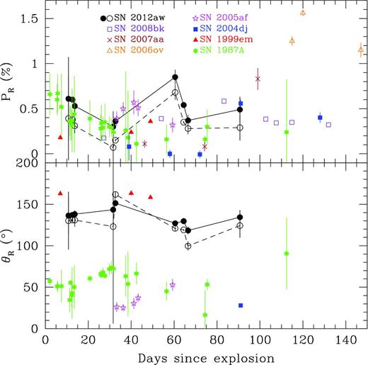
Comparison of polarization and PA values of SN 2012aw with those of other Type IIP SNe: SN 1987A, SN 1999em, SN 2004dj, SN 2005af, SN 2006ov, SN 2007aa and SN 2008bk. The upper and lower panels show the degree of polarization and PA, respectively. All values are intrinsic to a particular SN and symbols used in both panels are same. Thick and broken lines denote ISPMW and both ISPMW + ISPHG subtracted components, respectively, for SN 2012aw.
Shifting the phase (days after the explosion) by 21 d, the evolution of degree of polarization of SN 2004dj is very much similar to what has been seen in case of SN 2012aw as shown in the Fig. 6. However, it is important to mention that in case of SN 2004dj, the degree of polarization increases after the end of the plateau phase (when we see through the H-rich shell); whereas for SN 2012aw, the degree of polarization increases (around 60 d) during the plateau phase which could be a possible indication of a diverse nature of the two events. However, it is noticeable that like SN 2008bk, SN 2012aw is also strongly polarized well before the end of the plateau (see Leonard et al. 2012a), indicating a possible similarity in the both events. In the early phase (∼10–30 d), the ISPMW corrected PLC of SN 2012aw matches with that of the SN 1987A, whereas in the later phase (∼30–45 d) it is closely matching with that of SN 2005af. Nonetheless, it is worthwhile to mention that to derive the polarization parameters of SN 1987A and SN 2005af, the ISPHG components are not subtracted in respective studies. The polarimetric observations of SN 1999em are sparse; the polarization levels at different epochs seems to match with the ISPMW + ISPHG corrected PLC of SN 2012aw. It is also obvious from Fig. 6 that the polarization values of SN 2006ov remains more than 1 per cent for all three epoch observations which is higher than that of any of the Type IIP events in the list. Fig. 6 gives important information regarding the evolution of ejecta of similar types of SNe. By comparing the PLCs of various IIP SNe shown with different symbols in Fig. 6 (filled star: SN 1987A, filled triangle: SN 1999em, filled square: SN 2004dj, open star: SN 2005af, open triangle: SN 2006ov, cross: SN 2007aa, open square: SN 2008bk and for SN 2012aw symbols are the same as in Fig. 4), it could be conjectured that the properties of the ejecta from Type IIP SNe are diverse in nature as noticed by Chornock et al. (2010).
We have also compared the ISPMW and ISPHG corrected PLCs of SN 2012aw with those of other Type Ib/c CCSNe. Type Ib/c SNe are naturally more asymmetric in comparison to that of Type IIP SNe because they lack a thick He blanket that smear out the internal geometry. Therefore, a higher degree of polarization is observed in case of Type Ib/c SNe. In the present analysis, PLC of SN 2012aw is also clearly showing a lower degree of polarization in comparison to well-studied various Type Ib/c CCSNe (e.g. SN 2007uy, SN 2008D; Gorosabel et al. 2010). However, it is important to note that the PR peak value for SN 2012aw seen at ∼60 d is slightly less than the intrinsic polarization value of ∼1 per cent for the Type Ic SN 2008D which was related to violent X-ray transient (see Gorosabel et al. 2010). Here, it is noticeable that present PLC interpretations of SN 2012aw depend a lot on a single data point (May 15) which is significantly higher in the percentage polarization than the data taken at other epochs.
5 CONCLUSIONS
We present results based on nine epoch R-band imaging polarimetric observations of Type IIP supernova SN 2012aw. To the best of our knowledge, the initial three epoch polarimetric observations presented here are the earliest optical polarimetric data reported for this event. It was not possible to monitor the SN during the beginning of the nebular or post-nebular phase due to observational constraints; however, present observations cover almost up to the end of the plateau phase (∼90 d). The main results of our present study are the following:
The observed broad-band polarization for initial three epochs is ∼0.6 per cent, then decreases up to ∼0.3 per cent following a sudden increase up to ∼0.9 per cent on 2012 May 15 and at later epochs it seems to show a declining trend. However, the observed PA is almost constant, superimposed with slight variations.
To study the intrinsic polarization properties of SN 2012aw, we subtracted the contribution due to ISPMW and ISPHG from the observed P and θ values of SN. The ISPMW component was determined using the polarimetric observations of 10 field stars distributed within 10° radius around SN and located beyond 100 pc distance. The estimated Stokes parameters of ISPMW are found to be |$\langle Q_{\it {\rm ISP}_{\it {\rm MW}}}\rangle$| = −0.154 ± 0.002 per cent and |$\langle U_{\it {\rm ISP}_{\it {\rm MW}}}\rangle$| = 0.032 ± 0.002 per cent (equivalent to |$\langle P_{\it {\rm ISP}_{\it {\rm MW}}}\rangle$| = 0.157 ± 0.002 and |$\langle \theta _{\it {\rm ISP}_{\it {\rm MW}}}\rangle$| = 84| $_{.}^{\circ}$|10 ± 0| $_{.}^{\circ}$|43). We also estimated the degree of polarization (0.23 per cent) and PA (147°) at the location of SN by using the extinction value from the Schlegel map assuming that the host galactic dust follow the mean polarization efficiency and the magnetic field in the host galaxy follow the structure of the spiral arms.
The intrinsic polarization parameters of SN 2012aw follow trends of the photometric LC which could be attributed to the small-scale variations in the SN atmosphere or their interaction with the ambient medium.
Polarimetric parameters of this SN are compared with other well-studied Type IIP events. During the early phase (∼10-30 d), the ISPMW subtracted PLC of SN 2012aw matches with that of SN 1987A whereas at later epochs (∼30-45 d) it matches to that of SN 2005af.
ACKNOWLEDGEMENTS
The authors thank the anonymous referee for his/her critical review and constructive suggestions that helped to improve the contents and presentation of the paper. We are grateful to the observers Archana Soam, Manoj Kumar Patel and Ram Kesh Yadav at the Aryabhatta Research Institute of observational sciencES (ARIES) for their valuable time and support for the observations of this event. SBP and BK acknowledge the support of the Indo-Russian (DST-RFBR) project no. INT/RFBR/P-100 for this work. SBP also acknowledges Dr Koji S. Kawabata for useful discussions on various polarimetric aspects. CE acknowledges the financial support of the Pan-STARRS grant NSC 102-2119-M-008-001 funded by the Ministry of Science and Technology of Taiwan. JG acknowledges support of the Unidad Asociada IAA/CSIC-UPV/EHU and the Ikerbasque science foundation. This work has been supported by Spanish Junta de Andalucía through programme FQM-02192 and from the Spanish Ministry of Science and Innovation through Projects (including FEDER funds) AYA 2009-14000-C03-01 and AYA2008-03467/ESP. This research has made use of the SIMBAD data base, operated at CDS, Strasbourg, France. We acknowledge the usage of the HyperLeda data base (http://leda.univ-lyon1.fr).
http://leda.univ-lyon1.fr – Paturel et al. (2003).
Hubble Space Telescope.
Wide-Field and Planetary Camera 2.
Very Large Telescope.
Infrared Spectrometer And Array Camera.
New Technology Telescope.
Infrared spectrograph and imaging camera.
iraf is the Image Reduction and Analysis Facility distributed by the National Optical Astronomy Observatories, which are operated by the Association of Universities for Research in Astronomy, Inc., under cooperative agreement with the National Science Foundation.
