


Abstract
The understanding of the accelerated expansion of the Universe poses one of the most fundamental questions in physics and cosmology today. Whether or not the acceleration is driven by some form of dark energy, and in the absence of a well-based theory to interpret the observations, many models have been proposed to solve this problem, both in the context of General Relativity and alternative theories of gravity. Actually, a further possibility to investigate the nature of dark energy lies in measuring the dark energy equation of state (EOS), w, and its time (or redshift) dependence at high accuracy. However, since w(z) is not directly accessible to measurement, reconstruction methods are needed to extract it reliably from observations. Here, we investigate different models of dark energy, described through several parametrizations of the EOS. Our high-redshift analysis is based on the Union2 Type Ia supernovae data set (Suzuki et al.), the Hubble diagram constructed from some gamma-ray bursts luminosity-distance indicators, and Gaussian priors on the distance from the baryon acoustic oscillations, and the Hubble constant h (these priors have been included in order to help to break the degeneracies among model parameters). To perform our statistical analysis and to explore the probability distributions of the EOS parameters, we use the Markov Chain Monte Carlo Method. It turns out that, if exact flatness is assumed, the dark energy EOS is evolving for all the parametrizations that we considered. We finally compare our results with the ones obtained by previous cosmographic analyses performed on the same astronomical data sets, showing that the latter ones are sufficient to test and compare the new parametrizations.
1 INTRODUCTION
Since the end of the nineties, from observations on supernovae at high redshift, it is well known that the Universe is expanding. Pieces of evidence of scale temperature anisotropies in the cosmic microwave background (CMB) radiation have confirmed this result independently (Astier et al. 2006; Riess et al. 2007; Spergel et al. 2007; Kowalski et al. 2008; Planck Collaboration 2013). It is common practice to assume that the observed accelerated expansion is caused by dark energy, a presently dominant form of energy with unusual properties. The pressure of dark energy pde is negative and it is related to the positive energy density of dark energy ϵde by the equation of state (EOS) pde = wϵde, where the proportionality coefficient is such that w < 0. The nature of dark energy is still unknown, and we only know that it was estimated to be about 75 per cent of matter-energy in the Universe and that its properties are characterized by the EOS parameter, w. Extracting information on the EOS of dark energy from observational data is therefore a fundamental problem, but getting information from the observed data on such an EOS is at the same time both an issue of crucial importance and a challenging task. For probing the dynamical evolution of dark energy, under such circumstances, one can parametrize w empirically, by assuming, as usual, that this quantity evolves smoothly with redshift, so that it can be approximated by a fitting analytical expression, using two or more free parameters. Among all the possible parametrization forms of EOS, we will consider the Chevallier–Polarski–Linder (CPL) model (Chevallier & Polarski 2001; Linder 2003), which is widely used, since it presents a well-behaved and bounded behaviour for high redshifts, and a manageable two-dimensional parameter space. However, we will also introduce new parametrizations, that have been recently used by Ma & Zhang (2011) and Lazkoz, Salzano & Sendra (2010) to avoid the divergence problem inherent to the CPL parametrization, which turned out to be able to satisfy many theoretical scenarios. For constraining the parameters, which appear in the EOS, we use a large collection of cosmological data sets: the Union2 Type Ia supernovae (SNeIa) data set, the Hubble diagram constructed from some gamma-ray bursts (GRBs) luminosity-distance indicators, and in order to help break the degeneracies among model parameters, Gaussian priors on the distance from the baryon acoustic oscillations (BAOs), and the Hubble constant h. Actually, observations of the SNIa are consistent with the assumption that the observed accelerated expansion is due to a non-zero cosmological constant. However, so far the SNeIa have been observed only at redshifts z < 2, while in order to test if w is changing with redshift it is necessary to use more distant objects. New possibilities opened up when the GRBs have been discovered at higher redshifts, since this opened new avenues for cosmology, although they remain enigmatic objects. First of all, the mechanism that is responsible for releasing the incredible amounts of energy that a typical GRB emits is not yet known (see for instance Meszaros 2006 for a recent review). It is also not yet definitely known if the energy is emitted isotropically or is beamed. Despite these difficulties, GRBs are promising objects that can be used to study the expansion rate of the Universe at high redshifts (Bloom, Frail & Kulkarini 2003; Bradley 2003; Schaefer 2003, 2007; Dai, Liang & Xu 2004; Firmani et al. 2005; Amati et al. 2008; Amati, Frontera & Guidorzi 2009; Li et al. 2008; Tsutsui et al. 2009; Wang 2011a,b).
Actually, even if the huge dispersion (about four orders of magnitude) of the isotropic GRB energy makes them everything but standard candles, it has been recently empirically established that some of the directly observed parameters of GRBs are correlated with their important intrinsic parameters, such as luminosity or total radiated energy. This has allowed us to derive some correlations, which have been tested and used to calibrate those relations, and to derive their luminosity or radiated energy from one or more observables, making it possible to construct a GRBs Hubble diagram. It has also been shown that such a procedure can be implemented without specifying the cosmological model; see, for instance, Demianski & Piedipalumbo (2011), Demianski, Piedipalumbo & Rubano (2011) and references therein. In our analysis, we use a GRB HD data set consisting of 109 high-redshift GRBs, which has been constructed from the Amati Ep, i-Eiso correlation (here Ep, i is the peak photon energy of the intrinsic spectrum and Eiso the isotropic equivalent radiated energy), applying a local regression technique to estimate, in a model-independent way, the distance modulus from the recently updated Union SNeIa data set. It turns out that this and the other data sets are sufficient for our aim of testing and comparing the new parametrizations.
The scheme of the paper is as follows. In Section 2. we describe the basic elements of the parametrizations of the considered EOS, while in Section 3, we introduce the observational data sets that are used in our analysis. In Section 4, we describe some details of our statistical analysis from three sets of data. In a general discussion of our results and conclusions in Section 5, we finally present some constrains on dark energy models that can be derived from our analysis.
2 DARK ENERGY PARAMETRIZATIONS
As already said, the discovery that the expansion rate of the Universe is apparently accelerated is one of the most significant events in the modern cosmology. Although seemingly consistent with our current concordance model, in which the source of the cosmic acceleration takes the form of the Einstein cosmological constant, the precision of current data is however not sufficient to rule out the possibility of an evolving component. The fact that the Λ cold dark matter (CDM) model can be only an approximation generally leads to look for some dynamical field with a repulsive gravitational force. Moreover, this could instead be indicating that the Copernican principle is wrong, and that radial inhomogeneity is responsible for the accelerated expansion (Clarkson 2012; Valkenburg et al. 2013, Paper I; Valkenburg et al. 2013, Paper II).
Thus, given a parametrized ansatz for D(z), it is possible to reconstruct the dark energy EOS from equation (1). (See for instance Saini et al. 2000; Sahni et al. 2003, and references therein, for a review, and Rubano & Scudellaro 2002; Daly & Djorgovski 2004; Clarkson & Zunckel 2010; Lazkoz, Salzano & Sendra 2012; Sahni et al. 2013 for an overview about critical topics and alternative model-independent approaches connected to the dark energy reconstruction techniques.) New and interesting prospectives to extract information of the dark energy modelling based on a recent approach, the so-called genetic algorithms, are illustrated in Nesseris & Garcia-Bellido (2012), di Serafino et al. (2010) and di Serafino & Riccio (2010). Here, we are investigating if, by analysing a large collection of cosmological data, any indications of a deviation from the w(z) ≠ −1 come to light, as we have in fact detected in a previous cosmographic analysis, where the value of the deceleration parameter clearly confirmed the present acceleration phase, and the estimation of the jerk reflected the possibility of a deviation from the ΛCDM cosmological model. To accomplish this task, we focus on a direct and full reconstruction of the dark energy EOS through several parameterizations, widely used in the literature.
2.1 Basic equations
- The so-called CPL model (Chevallier & Polarski 2001; Linder 2003).This parametrization assumes a dark energy EOS given bywhere w0 and wa are real numbers that represent the EOS present value and its overall time evolution, respectively (Chevallier & Polarski 2001; Linder 2003). It is important to remember that for high redshifts we have the following behaviour:(9)\begin{equation} w(z) =w_0 + w_{1} z (1 + z)^{-1} \,, \end{equation}that allows us to describe a wide variety of scalar-field dark energy models. Then, this parametrization appears to be a good compromise to construct a model-independent analysis.(10)\begin{equation} \lim _{z \rightarrow \infty }w^{{\rm CPL}}(z)=w_0+w_a =: w_i^{{\rm CPL}} \end{equation}
- A novel parametrization recently introduced in Ma & Zhang (2011) to avoid the future divergence problem of the CPL parametrization, and to probe the dynamics of dark energy not only in the past evolution but also in the future evolution,(11)\begin{equation} w(z)=w_0+w_1 \left[\frac{\sin (z+1)}{z+1}-\sin (1)\right]. \end{equation}
- An oscillating dark energy EOS recently discussed in Lazkoz et al. (2010),These oscillating models have been proposed to solve the so-called coincidence problem very easily, due to the sequence of different periods of acceleration, and are available in several theoretical scenarios.(12)\begin{equation} w(z)=\frac{w_1 \left[1-\cos (\delta \log (z+1))\right]}{\log (z+1)}+w_0\,. \end{equation}
3 OBSERVATIONAL DATA SETS
As said, in our approach we use a great collection of presently available observational data sets on SNeIa and GRB Hubble Diagrams, and we set Gaussian priors on the distance from the BAOs, and the Hubble constant h.
3.1 SNeIa Hubble diagram
3.2 GRBs Hubble diagram
GRBs are visible up to high z, thanks to the enormous energy that they release, and thus may be good candidates for our high-redshift cosmological investigation. Sadly, GRBs may be everything but standard candles since their peak luminosity spans a wide range, even if there have been many efforts to make them standardizable candles using some empirical correlations among distance dependent quantities and rest-frame observables (Amati et al. 2008). These empirical relations allow one to deduce the GRB rest-frame luminosity or energy from an observer frame measured quantity so that the distance modulus can be obtained with an error which depends essentially on the intrinsic scatter of the adopted correlation.
Combining the estimates from different correlations, Schaefer (2007) first derived the GRBs HD for 69 objects, which has been further enlarged using updated samples, different calibration methods and also different correlation relations, see for instance Demianski & Piedipalumbo (2011), Demianski, Piedipalumbo & Rubano (2011), showing the interest in the cosmological applications of GRBs. In this paper, we perform our cosmographic analysis using two GRBs HD data set, build up by calibrating the Amati Ep, i-Eiso relation.
3.2.1 The calibrated Amati GRBs Hubble diagram
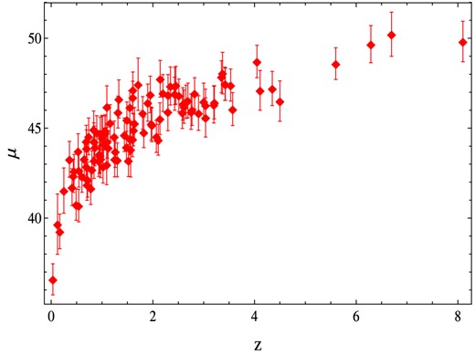
Distance modulus μ(z) for the calibrated GRBs Hubble diagram made up by fitting the Amati correlation.
3.3 BAOs data
4 STATISTICAL ANALYSIS
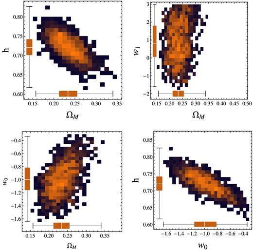
The joint probability for different couples of parameters which characterize the CPL EOS, as provided by our analysis. On the axes are plotted the box-and-whisker diagrams relatively to the different parameters: the bottom and top of the diagrams are the 25th and 75th percentile (the lower and upper quartiles, respectively), and the band near the middle of the box is the 50th percentile (the median).
Constraints on the EOS parameters for different parametrization. Columns report best-fitting (xbf), mean (〈x〉) and median (|$\tilde{x}$|) values and the 68 and 95 per cent confidence limits.
| Id | xbf | 〈x〉 | |$\tilde{x}$| | 68% CL | 95% CL |
|---|---|---|---|---|---|
| w(z) = w0 + w1z(1 + z)−1 | |||||
| ΩM | 0.225 | 0.238 | 0.237 | (0.206, 0.272) | (0.183, 0.305) |
| h | 0.732 | 0.714 | 0.713 | (0.68, 0.745) | (0.659, 0.778) |
| w0 | −1.15 | −0.832 | −0.834 | (−1.17, -0.476) | (−1.41, −0.36) |
| w1 | −0.99 | −1.06 | −1.05 | (−2.2, 0.037) | (−2.8, 0.74) |
| |$w_0+w_1 (\frac{\sin (z+1)}{z+1}-\sin (1))$| | |||||
| ΩM | 0.225 | 0.235 | 0.234 | (0.205, 0.264) | (0.182, 0.294) |
| h | 0.735 | 0.72 | 0.72 | (0.69, 0.75) | (0.66, 0.78) |
| w0 | −1.01 | −0.96 | −1.0 | (−1.23, −0.742) | (−1.43, −0.493) |
| w1 | 0.14 | 0.88 | 0.82 | (−0.27, 2.1) | (−1.18, 2.8) |
| |$w(z)=\frac{w_1 (1-\cos (\delta \log (z+1)))}{\log (z+1)}+w_0$| | |||||
| ΩM | 0.15 | 0.154 | 0.153 | (0.15, 0.21) | (0.13, 0.24) |
| h | 0.7 | 0.73 | 0.73 | (0.72, 0.75) | (0.7, 0.78) |
| w0 | −1.55 | −1.54 | −1.55 | (−1.59, −1.48) | (−1.66, −1.45) |
| w1 | 0.45 | 0.47 | 0.37 | (0.07, 0.78) | (0.013, 1.9) |
| δ | 0.76 | 0.66 | 0.62 | (0.54, 0.8) | (0.5, 1.1) |
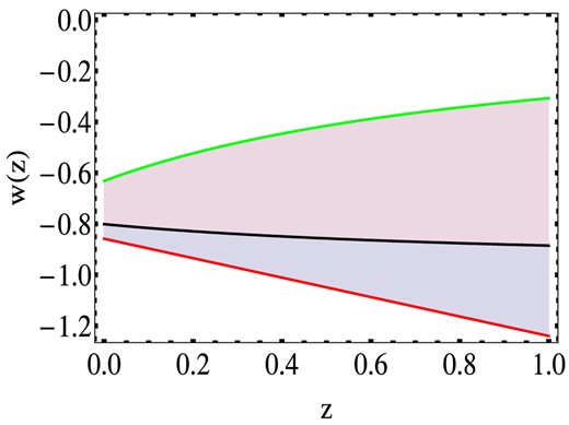
Redshift dependence of the CPL EOS for different values of the EOS parameters w0 and w1. The filled region corresponds to the allowed behaviour of the EOS, when the EOS parameters are varying within the 1σ range of confidence. Ωm is fixed and set to the best-fitting value. The solid black line corresponds to w0 = w0 bf, w1 = w1 bf.
In Figs 4 and 5, we show the behaviour of q0 as a function of w0 and the contour plots of j0 in the plane w0, w1, respectively. If we add to equations (34) and (35) the priors on the values of q0 and j0 obtained from the cosmographic analysis, it turns out that the range of confidence of the EOS parameters are squeezed at 1σ to w0 ∼ ∈(−0.87, −0.5) and w1 ∼ ∈(−0.3, 0.6). It is interesting to note, then, that the use of our large collection of present data sets, matched with the cosmographic analysis, allows us to improve the constraints on the dark energy EOS competitively with the improvements that can be achieved with future high-redshift SNeIa samples (see Salzano et al. 2013). Despite the remarkable improvements in the constraints on the EOS parameters, some caution is needed, due to the circumstance that the systems of algebraic equations in (16), and then their inverse, are highly non-linear. They admit multiple solutions for any assigned n-fold (q0, j0, s0, …), thus resulting in a strong degeneracy among the parameters, which is hard to manage. A possible strategy to ameliorate the maximum likelihood estimates could consist of incorporating the restrictions on the EOS parameters, coming from cosmography, in the likelihood itself. For this purpose, in a forthcoming paper we plan to implement at least two possibilities:
to use a constrained optimizer in maximizing the log-likelihood function,
to reparametrize the log-likelihood in such a way that the constraints are eliminated.
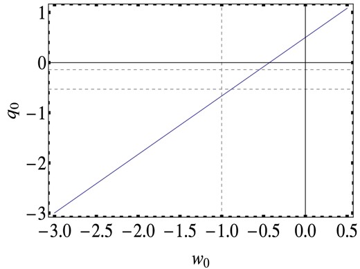
Behaviour of q0 as a function of w0 for Ωm = 0.237, as results from equation (34).The horizontal dashed lines correspond to the 2σ range of confidence for q0.
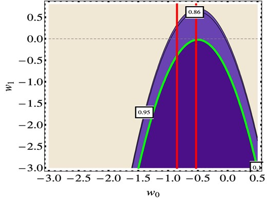
Contour plots of the jerk j0 in the plane w0, w1 for a CPL EOS parametrization, as provided by the cosmographic analysis. The value of Ωm is set at its median value Ωm = 0.237.
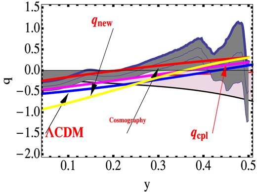
Reconstruction of deceleration history: the allowed region for q(z), obtained by Daly & Djorgovski, from the full data set is represented by the shadow area. The coloured solid line shows the deceleration function, q(z) for different EOS parametrization, as indicated by a label (the label new indicates the parametrization in equation 11). The red solid line shows the q(z) reconstruction obtained from the cosmography: it is interesting to note that it is all within the region allowed by the data.
4.1 Discussion
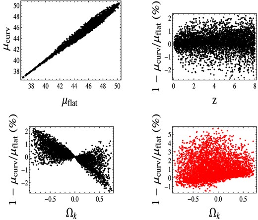
Percentage error on the modulus of distance with respect to a randomly generated Hubble diagram, in the case of a not flat cosmological model. As fiducial models, we consider a flat CPL quintessence (black points), and a flat ΛCDM (red points). In order to produce the μsimulated, ΩΛ, Ωk and the EOS parameters, w0 and w1 are variated. The Hubble constant is set at h = 0.68. The maximum relative dispersion is about 2 per cent for a flat CPL model, and reaches at most 4–5 per cent in the case of a ΛCDM model, even if unreasonable values of Ωk are allowed. It is worth noting that the GRBs Hubble diagram is ranked in the range of redshift where the dispersion reaches its own maximum (upper panel- right-hand side).
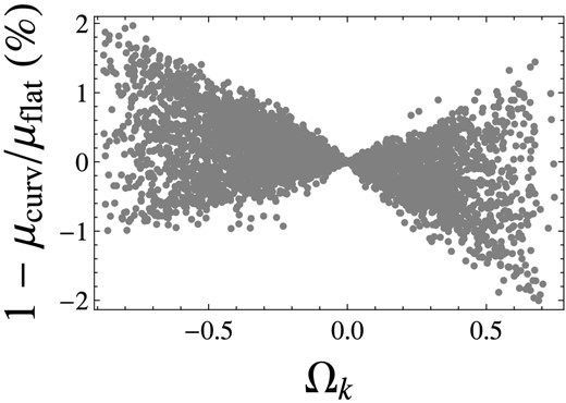
The percentage error as function of the curvature parameters in the case of a simulated SNeIa Hubble diagram for a flat CPL fiducial model.
It turns out that in the case of the simulated SNeIa Hubble diagram the scatter of the percentage error is further reduced. Moreover, we perform our analysis with the assumption of curvature included, limited to the CPL model. In order to test whether the statistical significance of our results is meaningfully overestimated by possible biases due to the GRBs calibration procedure (based on the SNeIa data set), we use GRBs only. We find that the main results of our analysis remain and
pieces of evidence for a time evolution of the EOS in such a parametrization are, indeed, confirmed;
the cosmological constant is not favourite, but is not ruled out from the analysis;
the very small value of Ωk is recovered.
Actually, it is worth noting that the GRBs Hubble diagram alone provides |$\Omega _{\rm k}^{{\rm median}}= -0.006$| and for the range of confidence at 1σ (−0.0073, 0.006), in agreement with the CMBR measurements. |$\Omega _{\rm m}^{{\rm median}}= 0.2465$|, and the 1σ confidence range is (0.157, 0.540). Moreover, for what it concerns the parameters of the EOS parametrization, it turns out that
the estimated w0 is shifted with respect to the flat case, being |$w_0^{{\rm median}} = -0.71$|, but the confidence range is rather stable, being (−1.05, 0.1);
w1 is weakly constrained, with |$w_1^{{\rm median}}=-0.24$| and the 1σ confidence range is rather stable, being (−1.05, 0.1).
This circumstance is not surprising, since the introduction of an additional dimension in the parameter space induced a strong degeneracy among Ωk, w0 and w1, as shown in Fig. 9, especially if the curvature density is restricted to the range allowed by the first cosmological Planck release, when the errors are actually dominated by the EOS.
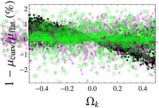
Comparison among the sensitivity of the modulus of distance |$\mu (z, \boldsymbol { \theta })$| on the curvature parameters (background black points), and the EOS parameters w0 and w1 (foreground magenta and green points, respectively). It is evidence of the strong degeneracy among Ωk, w0 and w1.
5 CONCLUSIONS
In this work, we have presented constraints on the dark energy EOS obtained by using an updated collection of observational data sets. In particular, we are looking for any indications of a deviation from the w(z) ≠ −1 come to light, reflecting the possibility of a deviation from the ΛCDM cosmological model. To accomplish this task, we focus on a direct and full reconstruction of the dark energy EOS through several parametrizations, widely used in the literature. We have found indications for a time evolution of the EOS in any considered parametrization, even if the cosmological constant is not ruled out from these observations. To discriminate between different models, we use the so-called BIC as selection criterion (Schwarz 1978): it turns out that the CPL parametrization is favoured by the data. Actually, we evaluated ΔBIC for each model, relative to the CPL model: it turns out that ΔBIC > 6, only for the 3D parametrization |$w(z)=\frac{w_1 (1-\cos (\delta \log (z+1)))}{\log (z+1)}+w_0$|, pointing out a strong evidence against this model. In the case of the oscillating EOS |$w_0+w_1 (\frac{\sin (z+1)}{z+1}-\sin (1))$|, we find out ΔBIC ≃ 5.9, underlying a certain (weak) positive evidence against such parametrization. It turns out that for the CPL parametrization |$w_0^{{\rm median}}=-0.834$|, and the range of confidence at 1σ is w0 ∼ ∈(−1.17, −0.476); |$w_1^{{\rm median}}=-1.05$| and w1 ∼ ∈(−2.2, 0.037). Moreover, it turns out that if we include in the space of parameters w0 − w1 the priors on the values of q0 and j0 obtained from the cosmographic analysis, the constraints on the EOS can be improved competitively with the improvements achieved with future high-redshift SNeIa samples: the range of confidence is, indeed, squeezed at 1σ to w0 ∼ ∈(−0.87, −0.5) and w1 ∼ ∈(−0.3, 0.6). However, since the map connecting the cosmographic and the EOS parameters is highly non-linear a strong degeneracy among the parameters is observed, which is hard to manage. Finally, we reconstruct the deceleration parameter q(z) for any considered EOS parametrization, comparing it with the q(z) obtained from observational data set, and with the cosmographicqcosmographic(z). It is interesting to note that just this qcosmographic(z) lies within the region allowed by the data, thus indicating that a possible strategy to ameliorate the EOS analysis and taking into the account the cosmography results, could consist of setting up a sort of constrained maximum likelihood estimate within the MCMCs, as we intend to perform in an upcoming paper. Finally, we also investigated whether and how strongly the constraints on the dark energy EOS change, if the curvature contribution is included in the analysis. We restricted our test to the CPL EOS, as exemplum. It turns out that, the main results are confirmed, and the ranges of confidence are stable, even if unreasonable values of Ωk are allowed. The main difference consists in the appearance of a strong degeneration among the cosmological parameters Ωk, w0 and w1. It is worth noting that the GRBs Hubble diagram provides as estimate for the curvature parameter |$\Omega _{\rm k}^{{\rm median}}= -0.006$|, and the 1σ confidence range is (−0.0073, 0.006), and |$\Omega _{\rm m}^{{\rm median}}=0.32$| in full agreement with the CMBR Planck measurements.
EP, MDL and PS acknowledge the support of INFN Sez. di Napoli (iniziativa Specifica CQSKY), and also EP and MDL acknowledge the support of INFN Sez. di Napoli (Iniziativa Specifica TEONGRAV). MDL is supported by MIUR (PRIN 2009).
