


Abstract
We investigate how the observed large-scale surface magnetic fields of low-mass stars (∼0.1–2 M⊙), reconstructed through Zeeman–Doppler imaging, vary with age t, rotation and X-ray emission. Our sample consists of 104 magnetic maps of 73 stars, from accreting pre-main sequence to main-sequence objects (1 Myr ≲ t ≲ 10 Gyr). For non-accreting dwarfs we empirically find that the unsigned average large-scale surface field is related to age as t−0.655 ± 0.045. This relation has a similar dependence to that identified by Skumanich, used as the basis for gyrochronology. Likewise, our relation could be used as an age-dating method (‘magnetochronology’). The trends with rotation we find for the large-scale stellar magnetism are consistent with the trends found from Zeeman broadening measurements (sensitive to large- and small-scale fields). These similarities indicate that the fields recovered from both techniques are coupled to each other, suggesting that small- and large-scale fields could share the same dynamo field generation processes. For the accreting objects, fewer statistically significant relations are found, with one being a correlation between the unsigned magnetic flux and rotation period. We attribute this to a signature of star–disc interaction, rather than being driven by the dynamo.
1 INTRODUCTION
Magnetic fields play an important role in stellar evolution. For low-mass stars, the magnetic field is believed to regulate stellar rotation from the early stages of star formation until the ultimate stages of the life of a star. In their youngest phases, the stellar magnetic field lines interact with accretion discs to prevent what would have been a rapid spin-up of the star, caused by accretion of material with high angular momentum and also the stellar contraction (e.g. Bouvier et al. 2013). After the accretion phase is over and the disc has dissipated, the contraction of the star towards the zero-age main sequence (ZAMS) provides an abrupt spin-up. From that phase onwards, ‘isolated’ stars (single stars and stars in multiple systems with negligible tidal interaction, such as the ones adopted in our sample) slowly spin-down as they age (e.g. Gallet & Bouvier 2013). This fact was first observed by Skumanich (1972, hereafter S72), who empirically determined that the projected rotational velocities v sin (i) of G-type stars in the main-sequence (MS) phase decrease with age t as v sin (i) ∝ t−1/2. This relation, called the ‘Skumanich law’, serves as the basis of the gyrochoronology method (Barnes 2003), which yields age estimates based on rotation measurements. The rotational braking observed by S72 is believed to be caused by stellar winds, which, outflowing along magnetic field lines, are able to efficiently remove the angular momentum of the star (e.g. Parker 1958; Schatzman 1962; Weber & Davis 1967).
Indicators of magnetic activity, such as surface spot coverage, emission from the chromosphere, transition region or corona, have been recognized to be closely linked to rotation (e.g. S72; Noyes et al. 1984; Vilhu 1984; Ayres 1997; Guedel 2007; Gondoin 2012; Reiners 2012). However, the magnetic activity–rotation relation breaks for rapidly rotating stars, where the indicators of stellar magnetism saturate and become independent of rotation. A saturation of the dynamo operating inside the star, inhibiting the increase of magnetism with rotation rate, has been attributed to explain the activity saturation observed in low-period stars (Vilhu 1984), but alternative explanations also exist (e.g. MacGregor & Brenner 1991; Jardine & Unruh 1999; Aibéo, Ferreira & Lima 2007).
The average unsigned surface magnetic field 〈|BI|〉, as measured by Zeeman-induced line broadening of unpolarized light (Stokes I), also correlates with rotation, in a similar way as the indicators of magnetic activity do (i.e. as one goes towards faster rotating stars, 〈|BI|〉 increases until it reaches a saturation plateau; Reiners, Basri & Browning 2009). Because 〈|BI|〉 is the product of the intensity-weighted surface filling factor of active regions f and the mean unsigned field strength in the regions BI (〈|BI|〉 = fBI), it is still debatable whether the saturation occurs in the filling factor f of magnetically active regions or in the stellar magnetism itself or in both (Solanki 1994; Saar 1996, 2001; Reiners et al. 2009).
Although Zeeman broadening (ZB) yields estimates of the average of the total (small and large scales) unsigned surface field strength, it does not provide information on the magnetic topology (Morin et al. 2013). For that, a complementary magnetic field characterization technique, namely Zeeman–Doppler imaging (ZDI; e.g. Donati & Brown 1997), should be employed. The ZDI technique consists of analysing a series of circularly polarized spectra (Stokes V signatures) to recover information about the large-scale magnetic field (its intensity and orientation). In this work, we take advantage of the increasing number of stars with surface magnetic fields mapped through the ZDI technique and investigate how their large-scale surface magnetism varies with age, rotation and X-ray luminosity (an activity index). In the past decade, ZDI has been used to reconstruct the topology and intensity of the surface magnetic fields of roughly 100 stars (for a recent review of the survey, see Donati & Landstreet 2009). Since the ZDI technique measures the magnetic flux averaged over surface elements, regions of opposite magnetic polarity within the element resolution cancel each other out (Johnstone, Jardine & Mackay 2010; Arzoumanian et al. 2011). As a consequence, the ZDI magnetic maps are limited to measuring large-scale magnetic field.
Because the small-scale field decays faster with height above the stellar surface than the large-scale field (e.g. Lang et al. 2014), only the latter permeates the stellar wind. If indeed magnetized stellar winds are the main mechanism of removing angular momentum from the star in the MS phase, one should expect the large-scale field to correlate with rotation and age. Likewise, a correlation between rotation and magnetism should also be expected if rotation is the driver of stellar magnetism through dynamo field generation processes. The interaction between magnetism, rotation and age is certainly complex and empirical relations, such as the ones derived in this work, provide important constraints for studies of rotational evolution and stellar dynamos.
This paper is organized as follows. We present our sample of stars in Section 2. Section 3 shows the empirically derived trends with magnetism we find within our data. In Section 4, we discuss how the results obtained using the ZB technique compare to the ones derived from ZDI (Section 4.1), we investigate the presence of saturation in the large-scale field (Section 4.2), analyse whether stars hosting hot Jupiters present different magnetism compared to stars lacking hot Jupiters (Section 4.3) and discuss the trends obtained for the pre-main-sequence (PMS) accreting stars (Section 4.4). In Section 5, we discuss the impact of our findings as a new way to assess stellar ages and as a valuable observational input for dynamo studies and stellar mass loss evolution. Our summary and conclusions are presented in Section 6.
2 THE SAMPLE OF STARS
The stars considered in this study consist of 73 late-F, G, K and M dwarf stars, in the PMS to MS phases. All have had their large-scale surface magnetic fields reconstructed using the ZDI technique, with some having been observed at multiple epochs, as listed in Table 1. The magnetic maps, 104 in total, have either been published elsewhere (Donati et al. 1999, 2003, 2008a,b,c, 2010a,b, 2011a,b,c, 2012, 2013; Marsden et al. 2006, 2011; Catala et al. 2007; Morin et al. 2008a,b, 2010; Petit et al. 2008, 2009; Fares et al. 2009, 2010, 2012, 2013; Hussain et al. 2009; Morgenthaler et al. 2011, 2012; Waite et al. 2011b; do Nascimento et al. 2013) or are in process of being published (Folsom et al., in preparation; Petit et al., in preparation; Waite et al., in preparation). Although the reconstructed maps provide the distribution of magnetic fields at the stellar surface, in this paper we only use the unsigned average field strengths 〈|BV|〉 (i.e. integrated over the surface of the star).1 In the present work, 〈|BV|〉 is calculated based on the radial component of the observed surface field, as we are mainly interested in the field associated with the stellar wind (Jardine et al. 2013). We also consider the Sun in our data set. For the solar magnetic field, we use the magnetograms from NSO/Kitt Peak data archive at solar maximum and minimum (Carrington rotations CR1851 and CR1907, respectively). To allow a direct comparison of the solar and stellar magnetic fields, we restrict the reconstruction of the solar surface fields to a maximum order of lmax = 3 of the spherical harmonic expansion (note, for instance, that modes with l ≲ 3 already contain the bulk of the total photospheric magnetic energy in solar-type stars; Petit et al. 2008).
The objects in our sample. Columns are the following: star name, spectral type, mass, radius, rotation period, Rossby number, age, X-ray luminosity, X-ray-to-bolometric luminosity ratio, average large-scale unsigned surface magnetic field and its observation epoch (year and month). The measurement errors associated with these quantities are described in Appendix A. References for the values compiled in this table are shown in the last column. In boldface are the references from which the ages adopted in this paper were obtained.
| Star | Sp. | M⋆ | R⋆ | Prot | Ro | Age | |$\log \left[\frac{L_{\rm X}}{\rm erg\,s^{-1}}\right]$| | |$\log \left[\frac{L_{\rm X}}{L_{\rm bol}}\right]$| | 〈|BV|〉 | Obs. | Ref. | |
|---|---|---|---|---|---|---|---|---|---|---|---|---|
| ID | type | (M⊙) | (R⊙) | (d) | (Myr) | (G) | epoch | |||||
| Solar-like stars | ||||||||||||
| HD 3651 | K0V | 0.88 | 0.88 | 43.4 | 1.916 | 8200 | 27.23 | −6.07 | 3.01 | − | 1,2,3 | |
| HD 9986 | G5V | 1.02 | 1.04 | 23.0 | 1.621 | 4300 | − | − | 0.517 | − | 1,2 | |
| HD 10476 | K1V | 0.82 | 0.82 | 16.0 | 0.576 | 8700 | 27.15 | −6.07 | 1.51 | − | 1,2,4 | |
| HD 20630 | G5Vv | 1.03 | 0.95 | 9.30 | 0.593 | 600 | 28.79 | −4.71 | 11.3 | 2012 Oct | 5,2,6,7 | |
| HD 22049 | K2Vk | 0.86 | 0.77 | 10.3 | 0.366 | 440 | 28.32 | −4.78 | 8.76 | − | 1,2,8,7 | |
| HD 39587 | G0VCH | 1.03 | 1.05 | 4.83 | 0.295 | 500 | 28.99 | −4.64 | 9.85 | − | 1,2,9,7 | |
| HD 56124 | G0 | 1.03 | 1.01 | 18.0 | 1.307 | 4500 | 29.44 | −4.17 | 1.81 | − | 1,2,10 | |
| HD 72905 | G1.5Vb | 1.00 | 1.00 | 5.00 | 0.272 | 500 | 28.97 | −4.64 | 7.49 | − | 1,2,9,7 | |
| HD 73350 | G5V | 1.04 | 0.98 | 12.3 | 0.777 | 510 | 28.76 | −4.80 | 5.86 | − | 1,2,11 | |
| HD 75332 | F7Vn | 1.21 | 1.24 | 4.80 | >1.105 | 1800 | 29.56 | −4.35 | 5.52 | − | 1,2,12 | |
| HD 76151 | G3V | 1.24 | 0.98 | 20.5 | − | 3600 | 28.34 | −5.23 | 5.05 | 2007 Jan | 13,14 | |
| HD 78366 | F9V | 1.34 | 1.03 | 11.4 | >2.781 | 2500 | 28.94 | −4.74 | 3.54 | 2011 | 15,1,4 | |
| ... | ... | … | … | … | … | … | … | … | 8.55 | 2008 | 15,1,4 | |
| ... | ... | … | … | … | … | … | … | … | 3.52 | 2010 | 15,1,4 | |
| HD 101501 | G8V | 0.85 | 0.90 | 17.6 | 0.663 | 5100 | 28.22 | −5.15 | 7.85 | − | 1,2,16 | |
| HD 131156A | G8V | 0.93 | 0.84 | 5.56 | 0.256 | 2000 | 28.86 | −4.44 | 11.9 | 2010 Jan | 17,2,1,7 | |
| ... | ... | … | … | … | … | … | … | … | 14.3 | 2009 Jun | 17,2,1,7 | |
| ... | ... | … | … | … | … | … | … | … | 11.6 | 2010 Aug | 17,2,1,7 | |
| ... | ... | … | … | … | … | … | … | … | 15.4 | 2010 Jun | 17,2,1,7 | |
| ... | ... | … | … | … | … | … | … | … | 14.1 | 2011 Jan | 17,2,1,7 | |
| ... | ... | … | … | … | … | … | … | … | 9.74 | 2008 Feb | 17,2,1,7 | |
| ... | ... | … | … | … | … | … | … | … | 20.1 | 2007 Aug | 17,2,1,7 | |
| HD 131156B | K4V | 0.99 | 1.07 | 10.3 | 0.611 | 2000 | 27.97 | −4.60 | 11.7 | − | 1,2,7 | |
| HD 146233 | G2V | 0.98 | 1.02 | 22.7 | 1.324 | 4700 | 26.80 | −6.81 | 0.969 | 2007 Aug | 13,18 | |
| HD 166435 | G1IV | 1.04 | 0.99 | 3.43 | 0.259 | 3800 | 29.50 | −4.08 | 10.9 | − | 1,2,19 | |
| HD 175726 | G5 | 1.06 | 1.06 | 3.92 | 0.272 | 500 | 29.10 | −4.58 | 6.85 | − | 1,2,20,21 | |
| HD 190771 | G5IV | 0.96 | 0.98 | 8.80 | 0.453 | 2700 | 29.13 | −4.45 | 13.4 | 2010 | 15,13,22 | |
| ... | ... | … | … | … | … | … | … | … | 6.45 | 2009 | 23,13,22 | |
| ... | ... | … | … | … | … | … | … | … | 4.50 | 2008 | 23,13,22 | |
| ... | ... | … | … | … | … | … | … | … | 6.80 | 2007 | 13,22 | |
| HD 201091A | K5V | 0.66 | 0.62 | 34.2 | 0.786 | 3600 | 28.22 | −4.53 | 2.68 | − | 1,2,24,25 | |
| HD 206860 | G0V | 1.10 | 1.04 | 4.55 | 0.388 | 260 | 29.00 | −4.65 | 14.7 | − | 1,2,26,14 | |
| Young suns | ||||||||||||
| BD-16 351 | K5 | 0.90 | 0.83 | 3.39 | − | 30 | − | − | 33.4 | 2012 Sep | 27,28 | |
| HD 29615 | G3V | 0.95 | 0.96 | 2.32 | 0.073 | 27 | − | − | 45.1 | 2009 | 29,30,31,28,32 | |
| HD 35296 | F8V | 1.22 | 1.20 | 3.90 | >0.467 | 35 | 29.43 | −4.41 | 8.37 | 2007 Jan | 29,2,33 | |
| ... | ... | … | … | … | … | … | … | … | 8.10 | 2008 Jan | 29,2,33 | |
| HD 36705 | K1V | 1.00 | 1.00 | 0.510 | 0.028 | 120 | 30.06 | −3.36 | 53.1 | 1996 | 34,35,36,37,38,7 | |
| HD 106506 | G1V | 1.50 | 2.15 | 1.39 | >0.024 | 10 | − | − | 30.8 | 2007 Apr | 39 | |
| HD 129333 | G1.5V | 1.04 | 0.97 | 2.77 | 0.177 | 120 | 29.93 | −3.60 | 47.9 | 2012 Jan | 29,2,37,38,7 | |
| ... | ... | … | … | … | … | … | … | … | 22.0 | 2007 Jan | 29,2,37,38,7 | |
| ... | ... | … | … | … | … | … | … | … | 29.3 | 2007 Feb | 29,2,37,38,7 | |
| ... | ... | … | … | … | … | … | … | … | 26.3 | 2006 Dec | 29,2,37,38,7 | |
| HD 141943 | G2V | 1.30 | 1.60 | 2.18 | >0.085 | 17 | − | − | 27.8 | 2009 Apr | 40 | |
| ... | ... | … | … | … | … | … | … | … | 45.8 | 2007 Mar | 40 | |
| ... | ... | … | … | … | … | … | … | … | 36.1 | 2010 Mar | 40 | |
| HD 171488 | G0V | 1.06 | 1.09 | 1.31 | 0.089 | 40 | 30.10 | −3.61 | 21.7 | 2004 Sep | 41,42,43 | |
| HII 296 | K3 | 0.80 | 0.74 | 2.61 | − | 130 | 29.33 | −3.85 | 36.6 | 2009 Oct | 27,44,45 | |
| HII 739 | G3 | 1.08 | 1.03 | 2.70 | − | 130 | 30.29 | −3.41 | 9.09 | 2009 Oct | 27,44,45 | |
| HIP 12545 | K6 | 0.58 | 0.57 | 4.83 | − | 21 | − | − | 78.5 | 2012 Sep | 27,46 | |
| HIP 76768 | K6 | 0.61 | 0.60 | 3.64 | − | 120 | − | − | 54.2 | 2013 May | 27,37,38 | |
| LQ Hya | K2V | 0.80 | 0.97 | 1.60 | 0.053 | 50 | 29.96 | −3.06 | 65.3 | 1998 Dec | 47,48,49 | |
| TYC0486-4943-1 | K3 | 0.69 | 0.68 | 3.75 | − | 120 | − | − | 20.1 | 2013 Jun | 27,37,38 | |
| TYC5164-567-1 | K2 | 0.85 | 0.79 | 4.71 | − | 120 | − | − | 39.4 | 2013 Jun | 27,37,38 | |
| TYC6349-0200-1 | K6 | 0.54 | 0.54 | 3.39 | − | 21 | − | − | 34.1 | 2013 Jun | 27,46 | |
| TYC6878-0195-1 | K4 | 0.65 | 0.64 | 5.72 | − | 21 | − | − | 31.7 | 2013 Jun | 27,46 | |
| Hot Jupiter hosts | ||||||||||||
| τ Boo | F7V | 1.34 | 1.42 | 3.00 | >0.732 | 2500 | 28.94 | −5.12 | 1.06 | 2008 Jan | 50,51,52,53 | |
| ... | ... | … | … | … | … | … | … | … | 1.81 | 2007 Jun | 54,51,52,53 | |
| ... | ... | … | … | … | … | … | … | … | 0.856 | 2006 Jun | 55,51,52,53 | |
| ... | ... | … | … | … | … | … | … | … | 0.925 | 2008 Jul | 50,51,52,53 | |
| HD 73256 | G8 | 1.05 | 0.89 | 14.0 | 0.962 | 830 | 28.53 | −4.91 | 4.38 | 2008 Jan | 51,57,56 | |
| HD 102195 | K0V | 0.87 | 0.82 | 12.3 | 0.473 | 2400 | 28.46 | −4.80 | 4.98 | 2008 Jan | 51,58,53 | |
| HD 130322 | K0V | 0.79 | 0.83 | 26.1 | 0.782 | 930 | 27.62 | −5.66 | 1.76 | 2008 Jan | 51,52,53 | |
| HD 179949 | F8V | 1.21 | 1.19 | 7.60 | >1.726 | 2100 | 28.61 | −5.24 | 1.53 | 2007 Jun | 59,51,52,53 | |
| ... | ... | … | … | … | … | … | … | … | 2.39 | 2009 Sep | 59,51,52,53 | |
| HD 189733 | K2V | 0.82 | 0.76 | 12.5 | 0.403 | 600 | 28.26 | −4.85 | 9.21 | 2008 Jul | 60,51,61,53 | |
| ... | ... | … | … | … | … | … | … | … | 9.23 | 2007 Jun | 60,51,61,53 | |
| M dwarf stars | ||||||||||||
| CE Boo | M2.5 | 0.48 | 0.43 | 14.7 | <0.288 | 130 | 28.40 | −3.70 | 91.6 | 2008 Jan | 62,44 | |
| DS Leo | M0 | 0.58 | 0.52 | 14.0 | <0.267 | 710 | 28.30 | −4.00 | 23.9 | 2007 Dec | 62,63 | |
| ... | ... | … | … | … | … | … | … | … | 27.4 | 2007 Jan | 62,63 | |
| GJ 182 | M0.5 | 0.75 | 0.82 | 4.35 | 0.054 | 21 | 29.60 | −3.10 | 73.6 | 2007 Jan | 62,46 | |
| GJ 49 | M1.5 | 0.57 | 0.51 | 18.6 | <0.352 | 1200 | 28.00 | −4.30 | 16.3 | 2007 Jul | 62,63 | |
| AD Leo | M3 | 0.42 | 0.38 | 2.24 | 0.047 | − | 28.73 | −3.18 | 152 | 2008 Feb | 64 | |
| DT Vir | M0.5 | 0.59 | 0.53 | 2.85 | 0.092 | − | 28.92 | −3.40 | 76.6 | 2008 Feb | 62 | |
| EQ Peg A | M3.5 | 0.39 | 0.35 | 1.06 | 0.020 | − | 28.83 | −3.02 | 282 | 2006 Aug | 64 | |
| EQ Peg B | M4.5 | 0.25 | 0.25 | 0.400 | 0.005 | − | 28.19 | −3.25 | 364 | 2006 Aug | 64 | |
| EV Lac | M3.5 | 0.32 | 0.30 | 4.37 | 0.068 | − | 28.37 | −3.32 | 406 | 2007 Aug | 64 | |
| GJ 1111 | M6 | 0.10 | 0.11 | 0.460 | 0.005 | − | 27.61 | −2.75 | 51.5 | 2009 | 65,66 | |
| GJ 1156 | M5 | 0.14 | 0.16 | 0.490 | 0.005 | − | 27.69 | −3.29 | 64.9 | 2009 | 65,10 | |
| GJ 1245B | M5.5 | 0.12 | 0.14 | 0.710 | 0.007 | − | 27.35 | −3.44 | 44.5 | 2008 | 65,10 | |
| OT Ser | M1.5 | 0.55 | 0.49 | 3.40 | 0.097 | − | 28.80 | −3.40 | 81.0 | 2008 Feb | 62 | |
| V374 Peg | M4 | 0.28 | 0.28 | 0.450 | 0.006 | − | 28.36 | −3.20 | 493 | 2006 Aug | 67,64 | |
| ... | ... | … | … | … | … | … | … | … | 554 | 2005 Aug | 67,64 | |
| WX UMa | M6 | 0.10 | 0.12 | 0.780 | 0.008 | − | 27.57 | −2.92 | 1580 | 2009 | 65,66 | |
| YZ CMi | M4.5 | 0.32 | 0.29 | 2.77 | 0.042 | − | 28.33 | −3.33 | 520 | 2007 Feb | 64 | |
| ... | ... | … | … | … | … | … | … | … | 480 | 2008 Feb | 64 | |
| Sun | ||||||||||||
| Max [CR1851] | G2V | 1.00 | 1.00 | 25.0 | 1.577 | 4600 | 27.67 | −5.91 | 3.81 | 1982 Jan | 68, 69 | |
| Min [CR1907] | G2V | 1.00 | 1.00 | 25.0 | 1.577 | 4600 | 26.43 | −7.15 | 1.89 | 1986 Mar | 68, 69 | |
| Classical T Tauri stars | ||||||||||||
| AA Tau | K7 | 0.70 | 2.00 | 8.22 | 0.036 | 1.4 | 30.08 | −3.50 | 918 | 2009 Jan | 70,71,72,73,74 | |
| BP Tau | K7 | 0.70 | 1.95 | 7.60 | 0.032 | 1.9 | 30.15 | −3.40 | 685 | 2006 Feb | 75,71,72,73,74 | |
| ... | ... | … | … | … | … | … | … | … | 654 | 2006 Dec | 75,71,72,73,74 | |
| CR Cha | K2 | 1.90 | 2.50 | 2.30 | 0.025 | 2.8 | 30.30 | −3.86 | 161 | 2006 Apr | 76,71,72,73,77 | |
| CV Cha | G8 | 2.00 | 2.50 | 4.40 | 0.079 | 4.8 | 30.11 | −4.36 | 170 | 2006 Apr | 76,71,72,73,78 | |
| DN Tau | M0 | 0.65 | 1.90 | 6.32 | 0.027 | 1.7 | 30.08 | −3.41 | 195 | 2012 Dec | 72,79,74 | |
| ... | ... | … | … | … | … | … | … | … | 317 | 2010 Dec | 72,79,74 | |
| GQ Lup | K7 | 1.05 | 1.70 | 8.40 | 0.042 | 3.4 | 29.87 | −3.71 | 600 | 2011 Jun | 80,71,72,73,81 | |
| ... | ... | … | … | … | … | … | … | … | 761 | 2009 Jul | 80,71,72,73,81 | |
| TW Hya | K7 | 0.80 | 1.10 | 3.56 | 0.020 | 9.6 | 30.32 | −2.80 | 885 | 2008 Mar | 82,71,72,73,81 | |
| ... | ... | … | … | … | … | … | … | … | 1120 | 2010 Mar | 82,71,72,73,81 | |
| V2129 Oph | K5 | 1.35 | 2.00 | 6.53 | 0.036 | 3.7 | 30.43 | −3.30 | 499 | 2005 Jun | 83,71,72,73,84 | |
| ... | ... | … | … | … | … | … | … | … | 644 | 2009 Jul | 83,71,72,73,84 | |
| V2247 Oph | M1 | 0.36 | 2.00 | 3.50 | 0.016 | 1.4 | 30.11 | −3.14 | 142 | 2008 Jul | 85,71,72,73,86 | |
| V4046 Sgr A | K5 | 0.95 | 1.12 | 2.42 | 0.021 | 16 | 30.08 | −3.11 | 69.1 | 2009 Sep | 87,71,72,73,88 | |
| V4046 Sgr B | K5 | 0.85 | 1.04 | 2.42 | 0.019 | 17 | 30.08 | −2.93 | 102 | 2009 Sep | 87,71,72,73,88 | |
1: Petit et al. (in preparation); 2: Marsden et al. (2013); 3: Canto Martins et al. (2011); 4: Katsova & Livshits (2006); 5: do Nascimento et al. (2013); 6: Ribas et al. (2010); 7: Wood, Laming & Karovska (2012); 8: Janson et al. (2008); 9: King et al. (2003); 10: Wright et al. (2011); 11: Plavchan et al. (2009); 12: Bruevich & Alekseev (2007); 13: Petit et al. (2008); 14: Pizzolato et al. (2003); 15: Morgenthaler et al. (2011); 16: Xing, Zhao & Zhang (2012); 17: Morgenthaler et al. (2012); 18: Guinan & Engle (2009); 19: Queloz et al. (2001); 20: Holmberg, Nordström & Andersen (2009); 21: Cutispoto et al. (2003); 22: Schmitt & Liefke (2004); 23: Petit et al. (2009); 24: Wood et al. (2002); 25: Mamajek & Hillenbrand (2008); 26: Eisenbeiss et al. (2013); 27: Folsom et al. (in preparation); 28: Torres et al. (2008); 29: Waite et al. (in preparation); 30: Waite et al. (2011a); 31: Messina et al. (2011); 32: Mentuch et al. (2008); 33: Guedel, Schmitt & Benz (1995); 34: Donati et al. (1999); 35: Strassmeier (2009); 36: Arzoumanian et al. (2011); 37: Barenfeld et al. (2013); 38: Luhman, Stauffer & Mamajek (2005); 39: Waite et al. (2011b); 40: Marsden et al. (2011); 41: Marsden et al. (2006); 42: Strassmeier et al. (2003); 43: Wichmann, Schmitt & Hubrig (2003); 44: Stauffer, Schultz & Kirkpatrick (1998); 45: Messina et al. (2003); 46: Binks & Jeffries (2014); 47: Donati et al. (2003); 48: Kovári et al. (2004); 49: Barrado y Navascués, Stauffer & Jayawardhana (2004); 50: Fares et al. (2009); 51: Fares et al. (2013); 52: Saffe, Gómez & Chavero (2005); 53: Poppenhaeger, Robrade & Schmitt (2010); 54: Donati et al. (2008a); 55: Catala et al. (2007); 56: Kashyap, Drake & Saar (2008); 57: Udry et al. (2003); 58: Ge et al. (2006); 59: Fares et al. (2012); 60: Fares et al. (2010); 61: Melo et al. (2006); 62: Donati et al. (2008c); 63: Vidotto et al. (2014); 64: Morin et al. (2008b); 65: Morin et al. (2010); 66: Schmitt, Fleming & Giampapa (1995); 67: Morin et al. (2008a); 68: Peres et al. (2000); 69: Bouvier & Wadhwa (2010); 70: Donati et al. (2010b); 71: Johnstone et al. (2014); 72: Siess et al. (2000); 73: Gregory et al. (2012); 74: Güdel et al. (2007); 75: Donati et al. (2008b); 76: Hussain et al. (2009); 77: Ingleby et al. (2011); 78: Feigelson et al. (1993); 79: Donati et al. (2013); 80: Donati et al. (2012); 81: Güdel et al. (2010); 82: Donati et al. (2011b); 83: Donati et al. (2011a); 84: Argiroffi et al. (2011); 85: Donati et al. (2010a); 86: Pillitteri et al. (2010); 87: Donati et al. (2011c); 88: Sacco et al. (2012).
Table 1 lists the general characteristics of the stars considered here, including quantities such as age t (whenever available), rotation period Prot, 〈|BV|〉, Rossby number Ro, X-ray luminosity LX and LX/Lbol, where Lbol is the bolometric luminosity. The measurement errors associated with these quantities are described in Appendix A. Among the 73 stars in our sample, 61 objects have age estimates (totalling 90 maps), which were collected from the literature and are based on different methods. For the PMS accreting stars, ages were derived using the stellar evolution models of Siess, Dufour & Forestini (2000), as derived in Gregory et al. (2012) and Donati et al. (2013). For the remaining stars, methods used for deriving ages include, for example, isochrones, lithium abundance, kinematic convergent point, gyrochronology, chromospheric activity. Note also that some of the stars in our sample are members of associations and open clusters and have, therefore, a reasonably well-constrained age (often derived with multiple methods). The last column of Table 1 lists the references for all the values adopted in this paper. In particular, the references from which ages were obtained are presented in boldface.
In order to investigate possible correlations in our data, we perform power-law fits of any two quantities x = log (X) and y = log (Y) (fitted through linear least-squares fits to logarithms), such that y = q + px (or Y = 10qXp), with q and p being the coefficients derived in the linear regression. These regressions were obtained using the bisector ordinary least-squares method (Isobe et al. 1990), which treats the x and y variables symmetrically (Jogesh Babu & Feigelson 1992). We opted such a fitting method because, for the quantities analysed here, the functional dependences of x and y are not clear.
Before we present the analyses of the trends with magnetism, it is useful to compare how our data relate to the Skumanich law, where rotation period Prot is related to age as Prot ∝ t1/2 or |$t \propto P_{\rm rot}^2$| (see Fig. 1). The power-law indices p obtained for the non-accreting (solid line) and accreting (dashed line) stars are shown in Table 2, along with the Spearman's rank correlation coefficient ρ and its probability under the null hypothesis (i.e. uncorrelated quantities). For the non-accreting stars, we find that |$t \propto P_{\rm rot}^{1.96 \pm 0.15 }$| (ρ = 0.76), which is consistent with the Skumanich law. Note that the accreting stars (green points) follow a different behaviour to the remaining objects in our sample and, because of that, we treat them as a different population throughout this paper. The physics of accreting stars is more complex than that of the discless stars, as the former interact with their accretion discs through stellar magnetic field lines that thread their discs (for a recent review see Bouvier et al. 2013 and references therein). As a consequence, the presence of the disc controls the rotation of these stars (Cieza & Baliber 2007). In addition, the young PMS stars will continue to contract once the disc has dispersed and, consequently, will spin-up, while evolving towards the ZAMS. Because not enough time has passed since their formation from the gravitational collapse of their natal molecular clouds, they still have imprinted on them the initial conditions of their rotation and, therefore, possess a large spread in the Prot–t diagram.
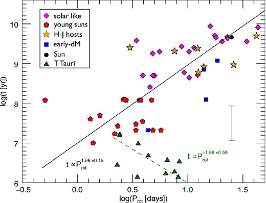
Correlation between age t and rotation period Prot for the stars in our sample, indicating that the non-accreting stars follow the Skumanich law (|$t \propto P_{\rm rot}^{2}$|). The solid (dashed) line is a power-law fit to our sample of non-accreting (accreting) objects. A typical error bar is indicated in grey (also in Figs 2–6).
Power-law indices (Y ∝ Xp) computed using the bisector linear least-squares method, fitted to logarithms. The Spearman's rank correlation coefficient ρ and its probability under the null hypothesis are also shown. Fits considering only non-accreting F, G, K and early-M dwarf stars, only PMS accreting stars and all the data in our sample are shown separately.
| Fits for dwarf stars only | Fits for accreting stars only | Fits considering all the sample | ||||||||
|---|---|---|---|---|---|---|---|---|---|---|
| Y | X | ρ | Prob. | p | ρ | Prob. | p | ρ | Prob. | p |
| (per cent) | (per cent) | (per cent) | ||||||||
| t | Prot | 0.76 | <0.01 | 1.96 ± 0.15 | −0.42 | 20 | −1.68 ± 0.59 | 0.66 | <0.01 | 2.54 ± 0.19 |
| 〈|BV|〉 | t | −0.79 | <0.01 | −0.655 ± 0.045 | −0.12 | 65 | −1.03 ± 0.42 | −0.87 | <0.01 | −0.701 ± 0.028 |
| ΦV | t | −0.81 | <0.01 | −0.622 ± 0.042 | −0.33 | 21 | −1.26 ± 0.35 | −0.89 | <0.01 | −0.840 ± 0.029 |
| 〈|BV|〉 | Prot | −0.54 | <0.01 | −1.32 ± 0.14 | 0.61 | 1.3 | 1.78 ± 0.49 | −0.44 | <0.01 | −1.72 ± 0.17 |
| ΦV | Prot | −0.72 | <0.01 | −1.31 ± 0.11 | 0.82 | <0.01 | 2.19 ± 0.43 | −0.57 | <0.01 | −2.06 ± 0.18 |
| 〈|BV|〉 | Ro | −0.80a | <0.01a | −1.38 ± 0.14a | 0.27 | 32 | 1.48 ± 0.81 | −0.91 | <0.01 | −1.325 ± 0.058 |
| ΦV | Ro | −0.71a | <0.01a | −1.19 ± 0.14a | 0.59 | 1.5 | 2.30 ± 0.74 | −0.88 | <0.01 | −1.596 ± 0.065 |
| LX | ΦV | 0.64 | <0.01 | 1.80 ± 0.20 | 0.20 | 46 | 0.70 ± 0.50 | 0.80 | <0.01 | 0.913 ± 0.054 |
| LX/Lbol | 〈|BV|〉 | 0.81 | <0.01 | 1.61 ± 0.15 | 0.059 | 83 | 1.01 ± 0.52 | 0.87 | <0.01 | 1.071 ± 0.067 |
| LX/Lbol | ΦV | 0.79 | <0.01 | 1.82 ± 0.18 | −0.23 | 38 | −0.92 ± 0.38 | 0.85 | <0.01 | 0.894 ± 0.055 |
aFits considering only points with Ro ≳ 0.1 (cf. Section 4.1).
3 TRENDS WITH MAGNETISM
In this section, we investigate possible trends between the following quantities: 〈|BV|〉, t, Prot, Ro, LX, LX/Lbol and unsigned magnetic flux ΦV. Table 2 summarizes the results of our fits. It is worth noting that, when analysed individually, each subset of objects (as presented in Table 1) does not show correlations with high statistical significance due to their narrow range of parameters (e.g. ages, rotation periods). However, trends are more robust when the different subsets are combined together and the dynamic range increases. For the non-accreting stars, all the relations have high statistical significance, with usually large Spearman's rank correlation coefficients and low probabilities of there not being correlations (<0.01 per cent). On the other hand, the relations we derive for the accreting stars are significantly poorer, with |ρ| ≲ 0.6 and usually high probabilities of these quantities not being correlated, except for ΦV versus Prot. The poorer fits are a result of the narrower range of parameters of this subset and also due to its relatively small number of data points (11 stars and 16 magnetic maps). These objects will be discussed in more detail in Section 3.2. Next, we discuss a few selected trends for the non-accreting population.
3.1 Non-accreting stars
3.1.1 Correlation with age
In his seminal paper, S72 predicted that magnetic fields decay as the inverse square of age, based on the age–rotation relation and further assuming that surface fields have a linear dependence with the rotation of the star (cf. Section 3.1.2). In order to test this prediction, we show in Fig. 2 the trend we find between 〈|BV|〉 and t for the stars in our sample. The correlation we found holds for more than two orders of magnitude in 〈|BV|〉 and three orders of magnitude in t for the non-accreting stars. From our power-law fit (solid line), we find that 〈|BV|〉 ∝ t−0.655 ± 0.045, which has a similar age dependence as the Skumanich law (Ω⋆ ∝ t−0.5) and supports the magnetism–age prediction inferred by S72 that there is magnetic field decay as the inverse square-root of age. A similar power-law dependence is found between the unsigned surface flux |$\Phi _V= \langle |B_V| \rangle 4 \pi R_\star ^2$| and age (ΦV ∝ t−0.622 ± 0.042).
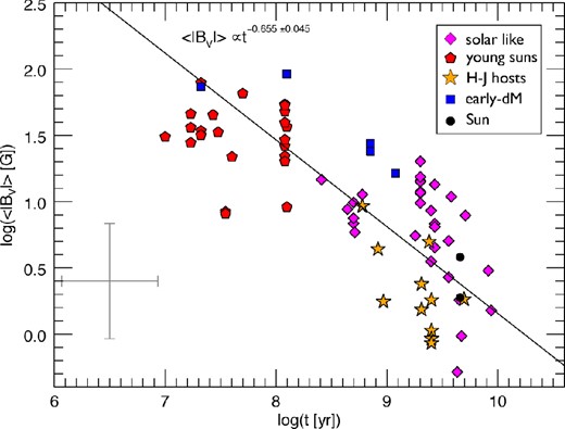
Correlation between the average large-scale field strength derived from the ZDI technique 〈|BV|〉 and age t, for the non-accreting stars in our sample. The trend found (solid line) has a similar age dependence as the Skumanich law (Ω⋆ ∝ t−0.5). This relation could be used as an alternative method to estimate the age of stars (‘magnetochronology’).
3.1.2 Correlation with rotation period
Stellar winds are believed to regulate the rotation of MS stars. The empirical Skumanich law, for example, can be theoretically explained using a simplified stellar wind model (Weber & Davis 1967), if one assumes that the stellar magnetic field scales linearly with the rotation rate of the star Ω⋆. To investigate whether our data support the presence of such a linear-type dynamo (|$B \propto \Omega _\star \propto P_{\rm rot}^{-1}$|), we present how 〈|BV|〉 scales with Prot in Fig. 3. Our results show that |$\langle |B_V| \rangle \propto P_{\rm rot}^{-1.32 \pm 0.14}$| (|ρ| = 0.54), indicating that our data support a linear-type dynamo of the large-scale field within 3σ. A similar nearly linear trend is found between the unsigned surface flux ΦV and Prot, with a larger correlation coefficient |ρ| = 0.72.
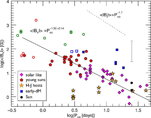
Correlation between the average large-scale field strength derived from the ZDI technique 〈|BV|〉 and rotation period Prot, for the non-accreting stars in our sample. Our data support the presence of a linear-type dynamo for the large-scale field (i.e. |$\langle |B_V| \rangle \propto \Omega _\star \propto P_{\rm rot}^{-1}$|) within 3σ, although a large scatter exists. The open symbols (not considered in the fit) are saturated M dwarf stars without age estimates: blue squares for M⋆ ≥ 0.4 M⊙ (early Ms), green circles for 0.2 < M⋆/M⊙ < 0.4 (mid Ms) and red circles for M⋆ ≤ 0.2 M⊙ (late Ms). The dotted line, at an arbitrary vertical offset, is indicative of the slope found from ZB measurements between 〈|BI|〉 and Prot (Saar 1996).
Although the correlation between 〈|BV|〉 and Prot indeed exists (with a negligible null probability), this relation has a significant spread. One possible explanation for this spread could be that in the Weber–Davis theory of stellar winds, a very simplistic field geometry is assumed (a split monopole) with the entire surface of the star contributing to wind launching. However, the complexity of the magnetic field topology can play an important role in the rotational evolution of the star (e.g. Vidotto et al. 2009, 2012; Cohen et al. 2010). ZDI observations have shown that stellar magnetic field topologies can be much more complex than that of a split monopole. In addition, numerical simulations of stellar winds show that part of the large-scale surface field should consist of closed field lines, which do not contribute to angular momentum removal (e.g. Vidotto et al. 2014). The large spread in the 〈|BV|〉–Prot relation could therefore be explained by the differences in magnetic field topologies present in the stars of our sample.
3.1.3 Correlation with Rossby number
Another possibility for the spread found in the relation between 〈|BV|〉 and Prot can be due to the fact that we are considering a broad range of spectral types. Traditionally, the use of Rossby number (Ro) instead of Prot allows comparison across different spectral types, reducing the spread commonly noticed in trends involving Prot. Ro is defined as the ratio between Prot and convective turnover time τc. To calculate Ro for the non-accreting stars, we used the theoretical determinations of τc from Landin, Mendes & Vaz (2010). Appendix A5 shows how our results vary if we adopt different approaches for the calculation of τc. For the eight stars that have masses outside the mass interval for which τc was computed in Landin et al. (2010, 0.6 ≤ M⋆/M⊙ ≤ 1.2), we adopt the following approximation. Stars with a given age t and mass M⋆ ≤ 0.6M⊙ were assumed to have τc = τc(M⋆ = 0.6 M⊙, t) and for M⋆ ≥ 1.2 M⊙ were assumed to have τc = τc(M⋆ = 1.2 M⊙, t). As a result, for the former (latter) group, the calculated τc is a lower (upper) limit, while Ro is an upper (lower) limit. In this work, we do not assign errors to Rossby numbers, but we note that these values are model dependent. For the accreting stars, Ro was derived from an update to the models of Kim & Demarque (1996), as detailed by Gregory et al. (2012).
In general, all our fits against Ro have larger unsigned Spearman's rank correlation coefficients than fits against Prot. Fig. 4(a) shows 〈|BV|〉 as a function of Ro, where we find that 〈|BV|〉∝Ro− 1.38 ± 0.14. This relation will be further discussed later on Section 4.1. Additionally, we found a similar power-law dependence between the magnetic flux ΦV and Ro (Fig. 4b): ΦV∝Ro− 1.19 ± 0.14. Right/left arrows in Fig. 4 denote the cases with lower/upper limits of Ro.
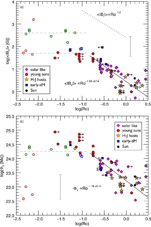
(a) Correlation between the average large-scale field strength derived from the ZDI technique 〈|BV|〉 and Rossby number Ro, for the non-accreting stars in our sample. Using Stokes I data, Reiners et al. (2009) showed that 〈|BI|〉 saturates for Ro ≲ 0.1. Donati et al. (2008c) suggested that there might be two different levels of saturation (dashed lines) among the low-mass stars, caused by different efficiencies at producing large- and small-scale fields. (b) Same as in (a), but now considering the magnetic flux ΦV. Note that the bi-modality in the saturation level is removed if ΦV is considered instead of 〈|BV|〉. Open symbols are as in Fig. 3. Solid lines show power-law fits considering objects with Ro ≳ 0.1. The dotted line (arbitrary vertical offset) in the upper panel is indicative of the slope found from ZB measurements between 〈|BI|〉 and Ro (Saar 2001).
We note that the correlation between 〈|BV|〉 and Ro indeed has less scatter than that between 〈|BV|〉 and Prot shown in Fig. 3. In spite of the tighter correlation, a noticeable scatter still exists, which, as discussed in Section 3.1.2, could be caused by different field topologies. It is also worth noting that the field topology and intensity can change over a stellar magnetic cycle and this fact alone can also be a source of scatter in our relations (although it is possibly not the dominant source). For the large-scale field of the Sun, a variation of a factor of ∼2 in 〈|BV|〉 is observed between the two maps used in this work, when the Sun changed to a simplified, large-scale dipolar topology at solar minimum (CR 1907) from a more complex one at maximum (CR 1851). For stars like HD 190711, the variation of 〈|BV|〉 among the maps considered in this study is almost a factor of 3.
3.1.4 Correlations with X-ray luminosity
Another interesting trend we found in our data is between the X-ray luminosity LX and ΦV (Fig. 5). For the non-accreting stars we found that |$L_{\rm X} \propto \Phi _V^{1.80 \pm 0.20}$|. If we include the accreting objects, the slope between LX and ΦV flattens and we find that |$L_{\rm X}^{\rm (all)} \propto \Phi _V^{0.913 \pm 0.054}$| (fit not shown in Fig. 5).
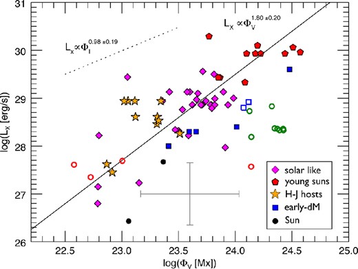
Correlation between X-ray luminosity LX and large-scale magnetic flux (|$\Phi _V=4\pi R_\star ^2 \langle |B_V| \rangle$|) derived from the ZDI technique for the non-accreting stars in our sample. The open symbols are as in Fig. 3 and were not considered in the fit (solid line). The dotted line, at an arbitrary vertical offset, is indicative of the slope found from ZB measurements for dwarf stars between LX and |$\Phi _I = {\langle |B_I| \rangle } 4 \pi R_\star ^2$| (Pevtsov et al. 2003). These slopes are consistent with each other within 3σ, but samples with a large dynamic range of 〈|BI|〉 are desirable to better constrain this result (see text).
We also investigate the trend between the ratio of X-ray-to-bolometric luminosity LX/Lbol and the large-scale magnetic field. Considering the dwarf stars represented by the filled symbols in Fig. 6, we found that LX/Lbol ∝ 〈|BV|〉1.61 ± 0.15 (solid line).
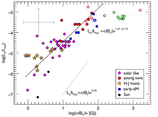
Correlation between the ratio of X-ray-to-bolometric luminosity (LX/Lbol) and large-scale magnetic field derived from the ZDI technique (〈|BV|〉) for the non-accreting stars in our sample. The open symbols are as in Fig. 3 and were not considered in our fit (solid line). The dashed line indicates the saturation plateau for Ro ≲ 0.1 at log (LX/Lbol) ≃ −3.1 (Wright et al. 2011). The dotted line, at an arbitrary vertical offset, is indicative of the slope found from ZB measurements (derived from results by Saar 2001; Wright et al. 2011).
3.2 Accreting PMS stars
Fig. 1 shows that the accreting stars form a different population compared to the discless stars. Besides the presence of the disc regulating the rotation of accreting PMS stars, they are also still contracting towards the ZAMS and, therefore, their radii and internal structures evolve considerably over a short time-scale (compared to their MS lifetime).
While the non-accreting stars show significant correlations in almost all the trends investigated in Table 2, the same is not true for the accreting stars. With the exception of the correlation between ΦV and Prot (discussed below), all the other trends investigated resulted in relatively low correlation coefficients and/or relatively high null probabilities (>0.01 per cent).
In accreting systems, the polar strength of the dipole component Bdip is particularly relevant for determining the disc truncation radius and the balance of torques in the star–disc system (e.g. Adams & Gregory 2012). Gregory et al. (2012) and, more recently confirmed by Johnstone et al. (2014), found that Bdip is correlated with Prot, such that stars with weak dipole components tend to be rotating faster than stars with strong dipole components. They attributed this correlation as a signature of star–disc interaction. Using the data for Bdip listed in Gregory et al. (2012), Donati et al. (2013) and Johnstone et al. (2014) together with the data presented in Table 1, we found that |$B_{\rm dip} \propto P_{\rm rot}^{2.05\pm 0.41}$|, with a Spearman's rank correlation coefficient of ρ = 0.83 and a probability of the null hypothesis that no correlation exists of ≪0.01 per cent. In addition, we also found that |$\Phi _V \propto B_{\rm dip}^{1.07 \pm 0.22}$| (ρ = 0.90). These two strong correlations directly explain the strong correlation reported in Table 2 between ΦV and Prot, where we found that |$\Phi _V \propto P_{\rm rot} ^{2.19\pm 0.43}$|, when the error in ΦV is properly accounted for. We caution, however, that these correlations are based on a small sample of accreting stars and more data are required for confirmation.
Accreting PMS stars with the simplest magnetic fields, and the largest magnetic flux, are therefore the slowest rotators. The correlations reported here are likely a manifestation of the star–disc interaction, as suggested by Gregory et al. (2012). Stars with more organized large-scale magnetospheres with stronger dipole components are able to truncate their discs at larger radii, where the Keplerian spin rate of the inner disc (and that of the star if they exist in a disc-locked state) is slower than it would be at the smaller truncation radii expected for stars with more complex magnetospheres with weaker dipole components. The latter sample of stars, with their lower magnetic flux ΦV, would therefore be faster rotators.2
Note that, because most PMS accreting stars observed to date have Ro ≪ 0.1 and are in the saturated regime, their dynamo-generated magnetic fields are not expected to depend on their rotation rates. The correlation between ΦV and Prot we observe is what we would expect if the rotation rates of accreting PMS stars are being dominated by star–disc interaction. In other words, the stellar magnetic field (via star–disc interaction) sets the rotation rate of accreting PMS stars, rather than the rotation rate setting the magnetic flux/strength through the dynamo field generation process. Or, at the very least, star–disc effects dominate any underlying dynamo relations at this early phase of stellar evolution.
4 DISCUSSION
4.1 Comparison between results from Zeeman broadening and Zeeman–Doppler imaging
In this section, we compare trends with magnetism. Stellar magnetic fields were obtained by two different techniques. The Zeeman-induced line broadening of unpolarized light (Stokes I), or ZB technique, yields estimates of the average of the total unsigned surface field strength (small- and large-scale structures), without providing information of the topology of the field. The ZDI technique (Stokes V), on the other hand, is able to reconstruct the intensity and topology of the stellar magnetic field, but cannot reconstruct the small-scale field component, which is missed within the resolution element of the reconstructed ZDI maps (Morin et al. 2013).3
These techniques are, nevertheless, complementary. The ZB technique is limited to slowly rotating objects (v sin (i) ≲ 20 km s−1), as broadening of spectral lines caused by rotation makes it more difficult to disentangle broadening caused by the Zeeman effect. The ZDI measurements, on the other hand, favour rapidly rotating objects (a few tens of km s−1, although recently ZDI measurements of more slowly rotating objects have become available). As a result, it is not always possible to obtain field measurements using both techniques for the same object (see Morin 2012, for a more in depth discussion). Because of that, in this section, instead of comparing results of both techniques on a case-by-case basis, we compare the results achieved from these techniques on samples of stars (which in general do not have overlapping members). The comparison presented next is summarized in Table 3. The dotted lines in Figs 3–6 indicate the slopes found from ZB measurements, assuming arbitrary vertical offsets.
Comparison between trends found using ZDI (this work) and ZB measurements for stars in the unsaturated regime. References for the latter are provided in the last column.
| From ZDI (this work) | From ZB | Reference |
|---|---|---|
| |$\langle |B_V| \rangle \propto P_{\rm rot}^{-1.32 \pm 0.14}$| | |$\langle |B_I| \rangle \propto P_{\rm rot}^{-1.7}$| | Saar (1996) |
| 〈|BV|〉∝Ro− 1.38 ± 0.14 | 〈|BI|〉∝Ro− 1.2 | Saar (2001) |
| |$L_{\rm X}^{\rm (all)} \propto \Phi _V^{0.913 \pm 0.054}$| | |$L_{\rm X}^{\rm (all)} \propto \Phi _I^{1.13}$| | Pevtsov et al. (2003) |
| |$L_{\rm X}^{\rm (dwarfs)} \propto \Phi _V^{1.80\pm 0.20}$| | |$L_{\rm X}^{\rm (dwarfs)} \propto \Phi _I^{0.98\pm 0.19}$| | Pevtsov et al. (2003) |
| LX/Lbol ∝ 〈|BV|〉1.61 ± 0.15 | LX/Lbol ∝ 〈|BI|〉2.25 | Saar (2001), Wright et al. (2011) |
Observations of magnetic fields of about a dozen stars using ZB have revealed that |$\langle |B_I| \rangle \propto P_{\rm rot}^{-1.7}$| (Saar 1996) and, in terms of Rossby numbers, 〈|BI|〉∝Ro− 1.2 (Saar 2001). In both works, a mix of saturated and unsaturated stars is considered, which implies that if one were to only consider the stars in the unsaturated regime, the slopes would be steeper than the ones derived by Saar (1996, 2001). Using the ZDI measurements of the large-scale field 〈|BV|〉, we found for the non-accreting stars that |$\langle |B_V| \rangle \propto P_{\rm rot}^{-1.32 \pm 0.14}$| and 〈|BV|〉∝Ro− 1.38 ± 0.14 (the latter considering only points with Ro ≳ 0.1, corresponding to the unsaturated stars). The similarities in the dependences of 〈|BI|〉 and 〈|BV|〉 with Prot and Ro might indicate that fields measured by ZDI (large scale) and ZB (large and small scale) are coupled to each other (see also Lang et al. 2014). This apparent coupling, therefore, might indicate that small- and large-scale fields share the same dynamo field generation processes, at least for stars in the unsaturated regime.
Another relevant comparison is the one between X-ray emission and magnetism as derived by ZB and ZDI (Fig. 5). Pevtsov et al. (2003) found that |$L_{\rm X}^{\rm (all)} \propto \Phi _I^{1.13\pm 0.05}$|, where |$\Phi _I = {\langle |B_I| \rangle } 4 \pi R_\star ^2$| is the unsigned magnetic flux derived from ZB. In this relation, Pevtsov et al. (2003) considered magnetic field observations of the Sun (quiet Sun, X-ray bright points, active regions and integrated solar disc), dwarf stars and PMS accreting stars, spanning about 12 orders of magnitude in magnetic flux. When we include all the objects in our sample, we found that |$L_{\rm X}^{\rm (all)} \propto \Phi _V^{0.913 \pm 0.054}$|, consistent to the nearly linear trend found by Pevtsov et al. (2003). When considering only the sample of 16 G, K and M dwarf stars (i.e. no solar data nor accreting PMS stars), Pevtsov et al. (2003) found that |$L_{\rm X}^{\rm (dwarfs)} \propto \Phi _I^{0.98\pm 0.19}$|, which is flatter than the correlation we found (|$L_{\rm X}^{\rm (dwarfs)} \propto \Phi _V^{1.80\pm 0.20}$|), based on a larger sample of 61 dwarf stars.4 Because of the relatively large errors in the power-law exponent of these relations, within 3σ they are still consistent with each other. This is a point worthy of further investigation. Finding a different power law for ΦV and ΦI may shed light on how the small- and large-scale field structures contribute to LX. By reducing the errors in the power-law fits (e.g. increasing the dynamic ranges of the fits, in particular in the ZB one), it would be possible to assess whether these relations are indeed consistent with each other.
Finally, in Fig. 6 we showed that LX/Lbol ∝ 〈|BV|〉1.61 ± 0.15 for the unsaturated stars. To the best of our knowledge, there is no such correlation constructed for 〈|BI|〉. We therefore combined the results of Saar (2001, 〈|BI|〉∝Ro− 1.2) and Wright et al. (2011, LX/Lbol∝Ro− 2.7 ± 0.13) to derive that LX/Lbol ∝ 〈|BI|〉2.25. Again, we note that the slope derived in Saar (2001) could be steeper if only the unsaturated stars were considered. Therefore, the slope of 2.25 we derive is an upper limit. Although we found a less steep dependence of LX/Lbol with 〈|BV|〉 than with 〈|BI|〉, given the uncertainties involved in the determination of these slopes, they can be considered consistent with each other. Unfortunately and in particular because of the small number of unsaturated stars with available 〈|BI|〉 measurements, it is still not possible to ascertain how large- and small-scale fields contribute to X-ray emission.
4.2 Saturation
Stars in the saturated regime show similar levels of X-ray-to-bolometric luminosity. In X-rays, saturation occurs for stars with Ro ≲ 0.1 (e.g. James et al. 2000; Pizzolato et al. 2003; Wright et al. 2011). In terms of their magnetism, there is evidence that the total field 〈|BI|〉 also saturates for Ro ≲ 0.1 (Reiners et al. 2009) and it would be interesting to investigate whether saturation is also present in the large-scale magnetic field 〈|BV|〉. In Fig. 4(a), we also present the remaining M dwarf stars, without age estimates (open symbols), collected from the samples in Donati et al. (2008c) and Morin et al. (2008b, 2010). They are in the X-ray saturated regime, with small Ro (Ro taken from Donati et al. 2008c; Morin et al. 2008b, 2010). It seems that these objects show different levels of saturation of 〈|BV|〉, with the mid-M dwarfs (green circles) saturating at log (〈|BV|〉/[G]) ∼ 2.6 while the early Ms (blue squares) at log (〈|BV|〉/[G]) ∼ 1.7 (horizontal dashed lines in Fig. 4a). Donati et al. (2008c) suggested that the step in the saturation level between early-Ms and mid-Ms is caused by different efficiencies at producing large-scale versus small-scale fields, where rapidly rotating mid-M dwarfs generate fields on larger spatial scales than early-M dwarfs (see also Reiners & Basri 2009, where a direct comparison between 〈|BV|〉 and 〈|BI|〉 was performed for a small sample of M dwarf stars). The saturation of late-M dwarfs (red circles), on the other hand, was shown to be divided into two distinct categories, either more similar to the saturation level of early-Ms or that of mid-Ms (Morin et al. 2010). Although in Donati et al. (2008c), Reiners & Basri (2009) and Morin et al. (2010) the three components of the reconstructed ZDI field were considered (radial, azimuthal and meridional) and in the present work we only focus on the radial component, the trends obtained in Fig. 4(a) are essentially the same as those discussed by these authors.
A unified saturation plateau for Ro ≲ 0.1 is observed if the magnetic flux ΦV is considered instead of the magnetic field intensity 〈|BV|〉 (Fig. 4b). This occurs at log (ΦV/[Mx]) ∼ 24.25. There is a spread in this plateau, in particular caused by the late-M dwarfs (red circles). This spread has also been observed in X-rays, for objects later than M6.5 (Cook, Williams & Berger 2014). The saturation of ΦV has not been recognized before. Observations of more objects at low Ro are desirable to provide better constraints on this saturation.
In Fig. 6, we investigated how LX/Lbol varied with magnetism. Overplotted to Fig. 6 are the remaining M dwarf stars, without age estimates (open symbols), from the samples in Donati et al. (2008c) and Morin et al. (2008b, 2010). The saturation value of log (LX/Lbol) = −3.13 ± 0.08, derived from the rotation–activity study performed by Wright et al. (2011), is shown as a dashed line. We see that the mid- and late-M dwarf stars approximately lie along this plateau. We did a similar analysis between LX/Lbol and magnetic flux ΦV and found that in this case, the plateau disappears as early- and mid-M dwarfs lie approximately along the same trend of LX/Lbol and ΦV as the remaining objects (|$L_{\rm X}/L_{\rm bol}\propto \Phi _V^{1.82 \pm 0.18}$|).
Fig. 7 shows a possible interpretation of our results, where we show a three-dimensional sketch of LX/Lbol, 〈|BV|〉 and Ro. In this sketch, Figs 4 (〈|BV|〉 versus Ro) and 6 (LX/Lbol versus 〈|BV|〉) are projections of a multidimensional distribution, as is the well-known relation between LX/Lbol and Ro. These projections are illustrated by dashed lines. According to our interpretation, the saturation plateau is actually a ‘plane’ (grey rectangular box), where objects of different internal structures (i.e. different masses) are located at different regions (drawn as blue stripes in our sketch). Each one of these stripes gives rise to the mass-dependent plateaus in the projected plane of {〈|BV|〉, Ro} (cf. Fig. 4) and it also accounts for the shift in 〈|BV|〉 observed for the mid-M dwarfs in the projected plane of {LX/Lbol, 〈|BV|〉} (cf. Fig. 6). The unsaturated stars consist of a tighter distribution of points (solid red stripe). In Fig. 7, we place our points in the three-dimensional space of {〈|BV|〉, Ro, LX/Lbol}, but it is worth noting that the activity relation is a function of other quantities as well, such as, age and mass.
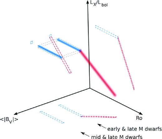
The activity relation is a complex function of many variables, such as age, mass, rotation and magnetism. Here we present a sketch in the three-dimensional space of {〈|BV|〉, Ro, LX/Lbol}, presenting a possible interpretation of how these quantities are related to each other (blue and red stripes). Figs 4 (〈|BV|〉 versus Ro) and 6 (LX/Lbol versus 〈|BV|〉) are projections of this multidimensional distribution, as is the well-known relation between LX/Lbol and Ro. These three projections are illustrated by dashed lines. The saturation plateaus seen in the projections form a saturation ‘plane’ (grey rectangular box) in the three-dimensional view, where objects of different masses are located at different regions (blue stripes).
4.3 Stars with hot Jupiters
Stars with close-in massive planets (or ‘hot Jupiters’, hJs) can experience strong tidal forces that may affect their rotation rates. It is believed that some stars that harbour hJs might have spun-up as a consequence of inward planetary migration (Lin, Bodenheimer & Richardson 1996; Gu, Lin & Bodenheimer 2003; Pont 2009; Brown et al. 2011). Among the stars in our sample, seven of them host hJs (12 ZDI maps shown as orange symbols in our figures). From Fig. 3, we note that these stars do not seem to have magnetic and rotation properties that differ from the remaining population of discless stars. Fares et al. (2013) also compared the large-scale magnetic topology of hJ-host stars adopted in our sample with that of stars without detected hJs and showed that both groups have similar magnetic field topologies.
Our findings suggest that the planets orbiting the hJ hosts in our sample might not be affecting significantly the rotation nor the large-scale magnetism of their host stars. A possible reason for this might be that tides in the systems analysed here are too weak to spin-up the host star (Lanza 2010) and, consequently, to change its magnetic properties. Alternatively, if these planets were at some point in the past able to affect the rotation of the star, the reaction of the dynamo should have occurred in a relatively short time-scale.
It is also worth pointing out that the hJ hosts seem to be systematically shifted towards lower 〈|BV|〉 values at a given age compared to solar-like stars (Fig. 2). This is likely to be a bias from planet search surveys, which prioritize targets with lower activity and, therefore, lower magnetism.
4.4 Accreting PMS stars
For accreting PMS stars, Johns-Krull (2007) found no correlation between any magnetic and stellar/dynamo parameters,5 and in particular, found no correlation between the magnetic flux ΦI, estimated from the average surface magnetic field as calculated from ZB measurements, and Prot. Out of the parameters that we have considered in Table 2, the only statistically significant correlation we have found for accreting PMS stars is between the magnetic flux ΦV, derived from the magnetic maps obtained through ZDI, and Prot. As discussed in Section 3.2, this is likely being driven by the star–disc interaction, which is controlled by the large-scale field topology probed with ZDI. ZB studies do not give access to the large-scale field topology, but are sensitive to the entirety of the stellar surface magnetic field, including the small-scale closed field regions that play no part in the star–disc interaction. The large-scale stellar magnetic field, in particular the dipole component Bdip of the multipolar magnetosphere, is the most important in terms of controlling the interaction with the disc (e.g. Adams & Gregory 2012; Gregory et al. 2012; Johnstone et al. 2014); Bdip can only be determined from ZDI studies. Therefore, the lack of correlation between ΦI and Prot does not pose a problem for our argument that the clear correlation between ΦV and Prot reported in this paper is driven by magnetic star–disc interaction.
5 MAGNETOCHRONOLOGY: MAGNETISM AS A NEW WAY TO ASSESS STELLAR AGE
One of our most interesting findings is the empirical trend between large-scale magnetism and age. Age is one of the most fundamental stellar parameters. However, the task of measuring ages is a very difficult one, with several methods having been used (see Soderblom 2010a; Soderblom et al. 2013, for recent reviews). For example, by solving the equations of the internal structure of the star, stellar evolution codes can be used as a tool to determine stellar age, from observational quantities, such as effective temperatures and luminosities. As in the MS phase, these parameters do not change significantly, isochrone dating is more unreliable for more evolved MS stars. The relation found between Prot and age first recognized by S72 has served as the basis of the gyrochronology method, which is able to provide stellar age estimates from rotation measurements (Barnes 2003; Barnes & Kim 2010). For young objects, the presence of lithium can constrain ages (Soderblom 2010b). Asteroseismology can also provide a means to derive stellar age (Christensen-Dalsgaard 1988; Otí Floranes, Christensen-Dalsgaard & Thompson 2005), although this method has been more widely applied to bright stars. Chromospheric activity can also be used as an astrophysical clock, although it seems to be more robust for objects with ages ≲2 Gyr (Pace 2013). The empirical relation that we identified between the large-scale magnetic fluxes and age (Fig. 2) can be used as an alternative method to estimate the age of stars. However, the relatively large spread of this correlation implies that this method, similarly to other age-dating methods, would carry significant imprecisions in age determination. Moreover, when compared to photometric measurements of rotation periods, the ‘magnetochronology’ method is more expensive in terms of observing time and field reconstruction than the gyrochronology method.
Our empirical trends are also relevant for investigations of rotational evolution of low-mass stars, as they provide important constraints on the evolution of the large-scale magnetism of cool stars, as well as their dependence on stellar rotation. For example, the relations 〈|BV|〉 versus t and 〈|BV|〉 versus Ro can be implemented in models investigating the evolution of mass and angular momentum loss (e.g. Gallet & Bouvier 2013). These relations also provide important constraints for stellar dynamo studies.
6 SUMMARY AND CONCLUSIONS
In this paper, we investigated how the large-scale surface magnetic fields of cool dwarf stars, reconstructed using the ZDI technique, vary with age, rotation period, Rossby number and X-ray luminosity. Our sample consists of 73 stars in the mass range between 0.1 and 2.0 M⊙ and spans about four orders of magnitude in age (from a Myr to almost 10 Gyr). As some of the stars have magnetic maps that were obtained at multiple observation epochs, our sample consists of 104 data points, including some PMS objects with on-going accretion. In order to separate the effects that accretion/PMS contraction might play on the rotational evolution of the stars, we have separated our sample into two populations.
For the population of accreting stars, we find few statistically significant correlations, except for the correlation between the unsigned magnetic flux ΦV and Prot (and between 〈|BV|〉 and the polar strength of the dipole component Bdip and ΦV versus Bdip). We attributed these correlations to a signature of star–disc interaction rather than being caused by the underlying dynamo field generation process.
For the population of non-accreting stars, we showed that their unsigned large-scale magnetic field strength 〈|BV|〉 is related to age t as 〈|BV|〉 ∝ t−0.655 ± 0.045, with a high statistical significance (Spearman's rank correlation coefficient of −0.79 and a very small null hypothesis probability). This relation presents a similar power dependence empirically identified in the seminal work of S72, which has served as the basis of the gyrochronology method to determine stellar ages from stellar rotation measurements. Our empirically derived magnetism–age relation could be used as a way to estimate stellar ages, although it would not provide better precision than the currently adopted methods.
Theoretically, S72's relation can be explained on the basis of the simplified wind model of Weber & Davis (1967), further assuming that a linear dynamo of the type |$B \propto \Omega _\star \propto P_{\rm rot}^{-1}$| is in operation. Empirically, we found that the large-scale unsigned surface field 〈|BV|〉 scales with the rotation period of the star as |$\langle |B_V| \rangle \propto P_{\rm rot}^{-1.32 \pm 0.14}$| or, in terms of Rossby number, 〈|BV|〉∝Ro− 1.38 ± 0.14. Our data, therefore, give support for a linear-type dynamo. Our empirically derived relations are relevant for investigations of rotational evolution of low-mass stars and give important observational constrains for stellar dynamo studies.
We also compared the trends we found in the ZDI data to trends empirically found using ZB measurements of magnetic field strengths 〈|BI|〉. For the unsaturated stars, the similar dependences of 〈|BI|〉 and 〈|BV|〉 with Prot and Ro indicate that fields measured by ZDI (large scale) and ZB (large and small scale) are coupled to each other. This might indicate that small- and large-scale fields share the same dynamo field generation processes. For the stars in the saturated regime, saturation of 〈|BI|〉 occurs for Ro ≲ 0.1 at 〈|BI|〉 ∼ 3 kG (Reiners et al. 2009, essentially for M dwarfs), while for 〈|BV|〉, saturation seems to have a bimodal distribution (Donati et al. 2008c) at 〈|BV|〉 ∼ 101.7 G for the early-Ms and at 〈|BV|〉 ∼ 102.6 G for the mid-Ms. We also found saturation of ΦV at ΦV ∼ 1024.25 Mx for Ro ≲ 0.1, but this is no longer bimodal as in the case of 〈|BV|〉. Observations of more objects at low Ro are desirable to provide better constraints on the saturation of ΦV.
We also investigate how the small- and large-scale structures contribute to X-ray emission (Figs 5 and 6). For the unsaturated stars, these contributions between X-ray emission and 〈|BV|〉 or 〈|BI|〉 have similar slopes within 3σ, but samples with large dynamic range of 〈|BI|〉 are required to better constrain this result.
The plots we presented in this paper could be understood as projections of a complex, multidimensional distribution, dependent on quantities such as LX/Lbol, 〈|BV|〉, rotation, age and internal structure. In Fig. 7, we offered a possible interpretation of this distribution in the three-dimensional space of {〈|BV|〉, Ro, LX/Lbol}. In this view, the unsaturated stars comprise a tight distribution of points, while the saturated objects give rise to a saturation ‘plane’ (instead of a plateau), where objects of different masses are located at different regions (shown as blue stripes in Fig. 7).
New near-infrared (NIR) spectropolarimeters, such as SPIRou (e.g. Delfosse et al. 2013), currently underconstruction for the Canada–France–Hawaii telescope, will be ideally suited for further comparison between the ZB and ZDI techniques. It will allow magnetically sensitive, Zeeman broadened, lines to be measured within the same spectra as used to reconstruct magnetic maps, thereby allowing a more direct comparison between 〈|BV|〉 and 〈|BI|〉.
AAV acknowledges support from a Royal Astronomical Society Fellowship and from the Swiss National Science Foundation via an Ambizione Fellowship. SGG acknowledges support from the Science and Technology Facilities Council (STFC) via an Ernest Rutherford Fellowship [ST/J003255/1] and RF via a consolidated grant [ST/J001651/1]. JB, PP and CPF acknowledge support from the ANR 2011 Blanc SIMI5-6 020 01 ‘Toupies: Towards understanding the spin evolution of stars’ (http://ipag.osug.fr/Anr_Toupies/). AAV would like to thank Professor Keith Horne and Dr Kate Rowlands for advice in the statistical analysis. NSO/Kitt Peak data used here are produced cooperatively by NSF/NOAO, NASA/GSFC and NOAA/SEL. Partly based on data from the Brazilian CFHT time allocation under the proposals 09.BB03, 11.AB05 (PI: do Nascimento Jr).
In order to differentiate between field strengths derived from Stokes V measurements (ZDI) and from Stokes I (ZB), we use the indices V and I, respectively.
If an accreting PMS is not locked to its disc, then a stronger dipole component allows the disc to be truncated at a larger radius, closer to corotation. This in turn means the star will experience smaller magnetic and accretion related spin-up torques (e.g. Bouvier et al. 2013 and references therein), and will more likely remain a slower rotator compared to a star with a weaker more complex magnetic field, as it evolves towards a disc-locked state.
The reconstructed fields are expressed as a spherical harmonic expansion. Note that the faster the rotation of the star, the larger is the spatial resolution. As a consequence, the ZDI reconstruction technique is able to recover magnetic fluxes at high order l of the spherical harmonics expansion for faster rotating objects (see Hussain et al. 2009, for a detailed analysis of the effects of resolution on what is recovered in the ZDI maps). In our sample, the maximum value of l varies from lmax ∼ 2 (e.g. for HD 76151; Petit et al. 2008) to ∼30 (e.g. for HD 141943; Marsden et al. 2011). To verify the existence of a possible bias in the reconstructed ZDI field with spatial resolution, we have recalculated 〈|BV|〉 for all the objects taking into account only the lowest orders of l. We adopted lcut-off = min (5, lmax) and recomputed the power-law indices p for all the relations presented in Table 2. The recalculated p are consistent within the fitting errors to what is presented in Table 2. The similarity between the relations when considering 〈|BV|〉(lcut-off) and 〈|BV|〉(lmax) is due to the fact that the largest powers in the harmonic expansions are in the low-l modes. This indicates that the different spatial resolution of the data considered here does not generate bias in the derived 〈|BV|〉 and, consequently, that our derived relations in Table 2 are robust.
Note that if we include the open symbols (M dwarf stars without age estimates) in the fit presented in Fig. 5, the slope we derive is slightly flatter (|$L_{\rm X}^{\rm (dwarfs)} \propto \Phi _V^{1.49\pm 0.17}$|), yet still consistent with the value quoted in the text.
Yang & Johns-Krull (2011) also found no correlations between the magnetic and dynamo parameters when considering PMS stars in the Orion nebula cluster (ONC), the TW Hydrae association and the same stars from Taurus considered by Johns-Krull (2007). A comparison of their sample of ONC stars with the catalogue of Hillenbrand et al. (1998) reveals it to be a mixture of both accreting and non-accreting PMS stars. However, Yang & Johns-Krull (2011) do find a reduction in ΦI with age which they attribute to the decrease in stellar radius as PMS contract towards the ZAMS. We do not find any statistically significant correlation between ΦV and age for our population of PMS stars (see Table 2). This may be because our sample size is too small (16 magnetic maps of 11 different accreting PMS stars) compared to the 31 stars considered by Yang & Johns-Krull (2011). Likewise, Johns-Krull (2007) found no correlation between ΦI and t in his smaller sample of 14 accreting PMS stars.
REFERENCES
APPENDIX A: ERROR ESTIMATES
In our fitting procedures, measurement errors were always accounted for. Typical error bars are indicated in the plots presented in this paper (grey error bars). In this appendix, we describe how the errors in the quantities plotted in this paper were estimated.
A1 Ages
The ages we adopted in this paper are listed in Table 1. They were compiled from different works in the literature and were derived by different methods. Although some of the ages of our stars are reasonably well constrained (e.g. some of our stars are members of associations and open clusters), most of them do not have assigned errors. In this paper, we have adopted a conservative error estimate of 0.434 dex in log t for all the stars in our sample. This is equivalent to adopting σt = t and accounts for the fact that the ages of older stars are in general more poorly constrained than the ages of younger ones.
A2 Magnetic field measurements
In the present work, the unsigned surface magnetic field strength 〈|BV|〉 and flux ΦV are calculated based on the radial component of the observed surface field. We have adopted in this paper a conservative error of |$\sigma _{\Phi _V}=\Phi _V$| and |$\sigma _{\langle |B_V| \rangle }=\langle |B_V| \rangle$|. This results in an error of about 0.434 dex in log (〈|BV|〉) and log (ΦV). Note that in the derivation of magnetic fluxes, we have not taken into consideration errors in the radii of stars.
We have also verified the effects of the spatial resolution on the field recovered by the ZDI technique, by artificially restricting the spherical harmonic expansion to low orders. We showed that the different spatial resolution of the data considered here does not generate bias in the derived 〈|BV|〉 and ΦV, and, consequently, that our derived relations are robust. More details of this analysis are provided in Footnote 3.
A3 X-ray luminosities
Because of coronal variability, it is likely that the values of LX presented in Table 1 are not the same as one would have derived if X-ray observations were to occur simultaneously with spectropolarimetric ones. For the Sun, it is observed that during its activity cycle, the X-ray luminosity varies from ≃ 0.27 to 4.7 × 1027 erg s−1 at minimum and maximum phases, respectively (Peres et al. 2000). This represents a variation of about 90 per cent from an average luminosity between these two extremes. Likewise, it is expected that stars also show X-ray variability during their cycles. To account for possible variations in LX over stellar cycles, we have assigned an error of 0.651 dex in log LX for all the objects in our sample, which is equivalent as assuming |$\sigma _{L_{\rm X}}=1.5L_{\rm X}$|.
A4 Rotation periods
Rotation periods are usually well constrained in the literature. In light of that and that errors are significantly larger for ages, magnetic fields and X-ray luminosities, we have neglected errors in rotation periods.
A5 Rossby numbers
In the literature, Rossby numbers Ro are usually preferred over rotation periods as they allow comparison across different spectral types, yielding tighter correlations (e.g. compare Figs 3 and 4). In this work, we did not assign errors to the computed Ro, but we caution that, to compute Ro, one needs to know the convective turnover time τc. To produce Fig. 4 and the results shown in Table 2, we adopted τc from Landin et al. (2010). Because we used the same model to compute Ro for all our non-accreting stars, these data points should have similar systematic errors.
However, we remind the reader that τc and, consequently, Ro are model-dependent quantities. To investigate the robustness of our relations against Ro for the non-accreting stars, we calculated Ro using two other different approaches. In the first approach, we interpolated from τc listed in Barnes & Kim (2010), derived for an age of 500 Myr. As the internal structure of the star does not change significantly after it has entered in the MS phase, τc should not change considerably, such that values listed by Barnes & Kim (2010) can still provide a reasonable estimate of Ro. In the second approach, we computed Ro using the empirical τc–M⋆ relation found by Wright et al. (2011).
Table A1 summarizes the power-law indices found when Ro was computed using τc from the models of Landin et al. (2010, LMV2010) and Barnes & Kim (2010, BK2010) and the empirically derived relation from Wright et al. (2011, W2011). The power-law indices derived from the theoretical models (LMV2010 and BK2010) are essentially identical within 1σ. Comparing these indices with the ones derived using the empirical determination of Ro (W2011), we again found reasonably good agreement (within 2σ). This shows that the relations we found against Ro are robust and, overall, are not significantly affected by the method adopted to derive τc.
Power-law indices p (Y ∝ Xp) computed by linear least-squares fit to logarithms for Rossby numbers calculated using different approaches: LMV2010 use the theoretical derivation of τc from Landin et al. (2010), BK2010 from Barnes & Kim (2010) and W2011 use the empirical derivation of τc from Wright et al. (2011). The fits only consider non-accreting F, G, K, M dwarf stars. In spite of the use of different relations to compute τc, all the fits are consistent with each other within 2σ.
| Y | X | LMV2010 | BK2010 | W2011 |
|---|---|---|---|---|
| 〈|BV|〉 | Ro | −1.130 ± 0.087 | −1.051 ± 0.084 | −1.41 ± 0.12 |
| ΦV | Ro | −1.143 ± 0.083 | −0.952 ± 0.095 | −1.31 ± 0.11 |
| Y | X | LMV2010 | BK2010 | W2011 |
|---|---|---|---|---|
| 〈|BV|〉 | Ro | −1.130 ± 0.087 | −1.051 ± 0.084 | −1.41 ± 0.12 |
| ΦV | Ro | −1.143 ± 0.083 | −0.952 ± 0.095 | −1.31 ± 0.11 |
SUPPORTING INFORMATION
Additional Supporting Information may be found in the online version of this article:
Table 1. The objects in our sample (machine-readable version) (Supplementary Data).
Please note: Oxford University Press is not responsible for the content or functionality of any supporting materials supplied by the authors. Any queries (other than missing material) should be directed to the corresponding author for the article.
