


Abstract
We present a new way of describing the flares from Sgr A* with a self-consistent calculation of the particle distribution. All relevant radiative processes are taken into account in the evolution of the electron distribution and resulting spectrum. We present spectral modelling for new X-ray flares observed by NuSTAR, together with older observations in different wavelengths, and discuss the changes in plasma parameters to produce a flare. We show that under certain conditions, the real particle distribution can differ significantly from standard distributions assumed in most studies. We conclude that the flares are likely generated by magnetized plasma consistent with our understanding of the accretion flow. Including non-thermal acceleration, injection, escape, and cooling losses produces a spectrum with a break between the infrared and the X-ray, allowing a better simultaneous description of the different wavelengths. We favour the non-thermal synchrotron interpretation, assuming the infrared flare spectrum used is representative. We also consider the effects on Sgr A*'s quiescent spectrum in the case of a density increase due to the G2 encounter with Sgr A*.
1 INTRODUCTION
1.1 Sagittarius A*
Sagittarius A* (Sgr A*) is the name given to the bright radio source of our Galactic Center. It was discovered in 1974 by Balick & Brown (1974) using the Green Bank 35 km radio link interferometer of the National Radio Astronomy Observatory. Stellar motion around the non-thermal radio source shows that Sgr A* is highly compact (smaller than 0.01 pc, i.e. 3 × 10¹¹ km) and that the stars orbit around a point mass of 4.3 ± 0.5 × 10⁶ M⊙ (Eisenhauer et al. 2005; Melia 2007). The stellar orbits provide the strongest evidence yet for a supermassive black hole located in the centre of our Galaxy at a distance of 8.3 ± 0.35 kpc (Reid 1993; Schödel et al. 2002; Ghez et al. 2008; Gillessen et al. 2009). Supermassive black holes (SMBHs) of millions to billions of solar masses are believed to exist in the centre of most galaxies. Sgr A*, in our own Galaxy, is the closest and best-studied SMBH, making it the perfect source to test our understanding of galactic nuclei systems in general. But among all galactic nuclei that we have observed so far, Sgr A* has the peculiarity of being very faint in all wavelengths. Even though it may have been more active in the past (Revnivtsev et al. 2004; Ponti et al. 2013; Zubovas & Nayakshin 2012), today Sgr A* is one of the most underluminous SMBHs we know, it is very faint with Lbol ≃ 10−9LEdd (Narayan et al. 1998) and accreting at a very low rate. The accretion rate has been constrained by polarization measurements, using Faraday rotation (Aitken et al. 2000; Bower et al. 2003; Marrone et al. 2007) and is estimated to be in the range |$2\times 10^{-9}<\dot{M}<2\times 10^{-7} \,\rm{M}_{{\odot }}\,{\rm yr^{-1}}$|. Theoretical work suggest that Sgr A* is most likely accreting at the lower range of this interval (Mościbrodzka et al. 2009; Drappeau et al. 2013). Dibi et al. (2012) have shown that for accretion rate above or equal to 1 × 10⁻⁸ M⊙ yr−1, the cooling losses become important in the modelling of the accretion flow and the resulting spectrum. This result means that Sgr A* is the only black hole source known where cooling could still be treated separately as a first approximation. Along the same lines, Yuan, Quataert & Narayan (2004) had shown that flare events, as these observed in the Galactic Centre, could not be detected if the accretion rate increases by a factor of 10 from its actual value, because synchrotron self-Compton (SSC) emission from thermal electrons would increases substantially. This would explain why Sgr A* is the only source known to exhibit flaring activity. Also, Yusef-Zadeh et al. 2009 are reporting observational evidence for IR flaring activity inversely proportional to the flux density.
1.2 Multiwavelength observations
The faint emission from Sgr A* has been observed in different wavelengths giving us a broad-band spectrum of this object from the radio to the X-ray (see reviews by Melia & Falcke 2001; Genzel, Eisenhauer & Gillessen 2010; Morris, Meyer & Ghez 2012, and references therein). From a few GHz up to 100 GHz, the radio spectrum extends as a rough power law Fν ∝ να with 0.25 ≤ α ≤ 0.33. Above 100 GHz there is evidence for a millimetre/sub-millimetre (sub-mm) excess over the power law, extending almost to 1000 GHz. The nature of this excess was discussed by Serabyn et al. (1997) and Falcke et al. (1998), who excluded the possibility of dust emission. The size of photosphere is predicted to be the smallest around this wavelength of 1.3 mm, where the excess is observed. And the black hole horizon, or its shadow (Falcke, Melia & Agol 2000; Dexter et al. 2010) could be detected for the very first time in the near future with new, very long base interferometry facilities such as the ‘Event Horizon Telescope’ (Doeleman et al. 2008, 2009; Fish et al. 2011).
Important progress has been achieved in the mid-infrared (MIR) to near-infrared (NIR; e.g. Genzel et al. 2003; Ghez et al. 2005; Schödel et al. 2011) and sub-mm domains. But in the optical and in the ultraviolet wavelengths, the Galactic Center is heavily obscured by gas and dust with 30 mag of visual extinction. This obscuring medium becomes partially transparent to the X-rays at energies above 2 keV. Indeed, Sgr A* has a quiescent X-ray luminosity of a few 1033 erg s−1 (Baganoff et al. 2003) which is about 1011 times lower than the Eddington luminosity.
Sgr A* is quite variable, and we observe fast activity (bursts or flares) in the infrared and X-ray band emissions. A few times a day, Sgr A* experiences rapid increases in the NIR flux (Hornstein et al. 2002; Genzel et al. 2003; Ghez et al. 2004; Eckart et al. 2006, 2008; Yusef-Zadeh et al. 2008; Dodds-Eden et al. 2011; Haubois et al. 2012), where brighter flares (>10 mJy; Dodds-Eden et al. 2011) are often associated with simultaneous X-ray flares (e.g. Baganoff et al. 2001; Goldwurm et al. 2003; Porquet et al. 2003, 2008; Bélanger et al. 2005; Nowak et al. 2012; Neilsen et al. 2013). The typical time-scale for such events is a few thousand seconds, suggesting a common localized origin of the flares. The radio and sub-mm emissions are more stable, i.e. they show less variability than the X-ray and NIR (see for instance Marrone et al. 2008 for the sub-mm flares, and Yusef-Zadeh et al. 2010 for a study on the IR–sub-mm anticorrelation). The flat radio emission is most likely the synchrotron emission originating from an outflow of Sgr A*, the lower the frequency, the further away we are in the outflow. So the radio wavelength, as well as the quiescent X-ray emission are coming from extended regions around Sgr A*, while the sub-mm, MIR, and flaring X-ray emissions originate from a region very close to the SMBH. This second region is the one we are interested in and we explore in this paper.
The MIR and NIR emission has been observed by the VLT and Keck (e.g. Bremer et al. 2011; Dodds-Eden et al. 2011; Schödel et al. 2011; Witzel et al. 2012). The X-ray variability has been observed by XMM–Newton, the Chandra X-ray observatory (e.g. Baganoff et al. 2001), and also by Swift (Degenaar et al. 2013). Many new X-ray flares have been detected recently, thanks to the Chandra 2012 Sgr A* X-ray Visionary Project.1 From this 3-Ms campaign, 39 X-ray flares are reported, lasting from a few hundred seconds to approximately 8 ks, and ranging in 2–10 keV luminosity from 1034 to 2 × 1035 erg s−1 (Nowak et al. 2012; Neilsen et al. 2013). The new telescope NuSTAR (Harrison et al. 2013) has released recently new X-ray flares data that we are using in our study (Barrière et al., submitted). Those show that the 3–80 keV emission is compatible with a pure power-law spectrum.
1.3 Flare models
The fast variability indicates that the origin of the flares is as close as a few gravitational radii from the SMBH. However, the nature of the physical processes responsible for the flares is still an open question. Different mechanisms have been proposed such as events of magnetic reconnection or other acceleration processes (e.g. Markoff et al. 2001; Yuan, Quataert & Narayan 2003; Liu, Petrosian & Melia 2004; Liu et al. 2006), infall of gas clumps or disruptions of small bodies (Cadež et al. 2006; Tagger & Melia 2006; Zubovas, Nayakshin & Markoff 2012), adiabatic expansion of hot plasma or hotspot models (Broderick & Loeb 2006; Yusef-Zadeh et al. 2008). By modelling the physical conditions around Sgr A* and fitting the observational data, we also aim at giving a possible interpretation of the phenomenon.
Several studies have been devoted to the modelling of SgrA* flares. Some models include a precise description of the flow geometry. For instance, the emission from SgrA* was interpreted in the framework of radiatively inefficient accretion flows (Yuan et al. 2003). In this model, the matter properties (density, temperature, etc.) are computed through hydrodynamical equations including radiative losses. These properties depend on the distance to the black hole and each ring contributes differently to the overall spectrum. The outer parts of the accretion flow contribute significantly to the X-ray luminosity in the quiescent state (Quataert 2002; Baganoff et al. 2003) with only about 10 per cent of the quiescent X-ray flux coming from the central part we are modelling (Neilsen et al. 2013; Wang et al. 2013).
However, even in models where the geometry is dealt with accuracy, most of the emission originates from the very central parts of the accretion flow, both in the quiescent sub-mm and NIR bands, and in the flaring sub-mm to X-ray bands. Moreover, the typical time-scale of a flare (a few thousand seconds, depending on the flare) is of the order of the orbital period at the innermost stable orbit of SgrA*, pointing again to a flaring region of only a few gravitational radii (rG = GM/c2). Therefore, most attempts to model the sub-mm to X-ray spectrum of SgrA* in the quiescent and flaring states (excluding the radio emission) implicitly assume that the emission originates from a single homogeneous, isotropic zone characterized by only few parameters such as the average electron temperature and density, the magnetic field intensity (e.g. Liu et al. 2006; Dodds-Eden et al. 2010). Here, we use the same approach.
Most models agree on the fact that the small emitting region is weakly magnetized (≲ a few hundred Gauss) and faint (≲108 particles cm−3) which now appear as standard values (Dexter, Agol & Fragile 2009; Mościbrodzka et al. 2009; Dibi et al. 2012). These values are supported by observations that constrain the accretion rate via Faraday rotation, to a maximum of |$\dot{M} \sim 10^{-7}$| M⊙ yr−1. As a simple check, taking this higher accretion rate limit and a ‘typical’ bulk velocity at one or two gravitational radii of 10 per cent of the speed of light (as simulated in general relativistic magnetohydrodynamics models of Sgr A*), then |$\rho _{\rm max} \simeq \dot{M}/(4 \pi R^2 v) \sim 10^8 \,{\rm particles\,cm}^{-3}$|.
Whatever the details of the accretion flow and the radiative processes responsible for the emission, the emitted spectrum depends drastically on the particle distribution. For the sake of simplicity, all models so far have assumed predetermined particle distributions (Maxwellian, power law, broken power law, or a combination of them) which are described by few parameters. The precise shape of the particle distributions depends on the radiative and acceleration processes and can deviate significantly from the assumed ones. This work aims at dealing more precisely with particle distributions. Fitting arbitrary distributions to the data is not possible with current coverage and sensitivity of the instruments. Rather, the shape of the particle distribution can be computed self-consistently with a Boltzmann equation assuming a physics described by a few parameters. Such an approach is common in the modelling of the high-energy emission from X-ray binaries and other AGN (e.g. McConnell et al. 2002; Rogers et al. 2006; Belmont, Malzac & Marcowith 2008) but has not been applied to SgrA* yet. In this paper, we present spectra obtained by solving simultaneously an equation for particles and an equation for photons to produce self-consistent particle distributions and spectra. These spectra are compared to broad-band data of SgrA* to put constraints on the flare properties.
This paper is organized as follows: In Section 2, we present the microphysics and numerical method. In Section 3, we present the results and solutions for the quiescent and flaring spectra from Sgr A*. We study the plasma behaviour in two kinds of models, namely in systems where matter is trapped in the emission region, and in systems where matter flows in and out of the emission region. In Section 4, we end with our conclusions and outlook.
2 METHOD
The goal of this study is to model the plasma around Sgr A*, and in particular the particle distributions and the resulting spectra. In the following, we will note ν the frequency of photons, γ the particles Lorentz factor, and p = (γ2 − 1)1/2 the particle momentum.
We use the belm code (Belmont et al. 2008). This numerical tool solves simultaneously coupled kinetic equations for leptons and photons in a magnetized, uniform, isotropic medium of typical size R. In all models presented here, this size is set to R = 2 rG = 1.3 × 1012 cm based on the size derived from the flare time-scale variability (where rG = GM/c2 is the gravitational radius).
The implemented microphysics includes radiation processes as self-absorbed radiation, Compton scattering, self-absorbed bremsstrahlung radiation, pair production/annihilation, Coulomb collisions, and prescriptions for particle heating/acceleration.
2.1 Radiative processes
The effect of self-absorbed bremsstrahlung radiation is also computed. However, for the innermost regions of the accretion flow, bremsstrahlung emission is a negligible component of the resulting spectra, and it will not be discussed in this paper.
Photon–photon pair production and pair annihilation are also implemented in the code. However, we aim at modelling the emission from SgrA* only below 100 keV where these processes are negligible. They were disabled in order to reduce the computation time.
Rather than computing the path of photons out of the emitting region with Monte Carlo simulations, photons produced in situ are assumed to escape with a probability representative of the geometry. This probability depends on the photon energy. For instance, high-energy photons do not inverse Compton scatter and can escape freely when the optical depth is large, low-energy photons can be scattered so much that they remain trapped in the system much longer. We use the escape rate from Lightman & Zdziarski (1987) and Coppi (2000) that reproduces well the results of Monte Carlo simulations in a spherical geometry. At low energy, synchrotron and bremsstrahlung can absorb photons before they escape. This modifies the escape probability in this energy range. We include the corresponding modifications to escape probability derived from Sobolev (1957, see also Poutanen & Vurm 2009).
2.2 Particle acceleration and heating
The particle distribution depends on the above-mentioned radiative processes and on several additional processes.
Coulomb collisions tend to thermalize the particle distributions. The belm code includes Coulomb cross-sections derived from Nayakshin & Melia (1998). However, the very low densities inferred for SgrA* make this process very inefficient. In all the results shown in this paper, real Coulomb collisions are completely negligible.
In order to account for the observed high-energy radiation, particles needs to be heated/accelerated to high energy. Solving for the particle distribution thus requires addressing also the physics of particle acceleration/heating. Many processes have been proposed to account for high-energy particles (viscosity, reconnection, shocks, first- and second-order Fermi processes, etc.). However, the precise process at work in SgrA* is still unknown. Moreover, the physics of these processes is not constrained well enough construct precise models for their effect on the particle distribution. Only stochastic acceleration by magnetohydrodynamic (MHD) waves can be implemented easily in a Boltzmann equation for the particle distribution (see Liu et al. 2006 for an application to SgrA*). However, if particle escape is slow, it forms a quasi-Maxwellian distribution and does not reproduce hard non-thermal distributions, such as the one observed by NuSTAR. If particle escape is efficient, it can produce power laws only if the accelerating rate has the same energy dependence as the radiative cooling, which is very unlikely (Katarzyński et al. 2006b). Therefore, we use very general, ad hoc prescriptions, inspired from what is done for the corona of accreting black holes (such as eqpair; Coppi 2000; or belm). We use two different channels to provide energy to the particles.
We mimic thermal processes by computing Coulomb collisions with a virtual population of hot protons (with temperature kBTp = 40 MeV). Real collisions are very inefficient and do not provide significant heating, whatever the proton temperature. Rather, this prescription aims at reproducing the effect of anomalous processes (such as viscosity) on the lepton distribution. Therefore, the heating efficiency is renormalized by an arbitrary constant so that to inject power Lth (erg s−1) into the emitting region. In the following, this free parameter will be described by the compactness parameter lth = σTLth/(Rmec3). Such prescription not only heats the global distribution of particles. It also thermalizes it. As the efficiency of the virtual collisions is enhanced, the efficiency of the associated thermalization is also enhanced to an anomalous level. Anomalous heating is a common feature of accreting systems, so such heating is not surprising even though the origin is debatable.
We model non-thermal processes by constantly injecting particles with a power-law distribution N(γ) ∝ γ−s. This distribution is characterized by four parameters: the slope s, the minimal and maximal energies γmin and γmax, respectively, and the normalization. As we want this process to keep the number of particles constant, the reinjected particles are taken from the lepton population itself, with a uniform probability, independent of their energy. In the following, the minimal energy of the power law will be set to γmin = 50, so that particles are accelerated from the bulk of the distribution. Indeed, the thermal peak of the spectrum (around 1012 Hz) imply an electron temperature around 1011 K. And the maximal energy of accelerated particles will be set to γmax = 4.6 × 10⁵, large enough to reproduce the NuSTAR data. The high-energy cutoff has not been confirmed by NuSTAR observations (Barrière et al., submitted), and the possible physical processes responsible for the non-thermal component (turbulent acceleration, reconnection, weak shocks) can accelerate electrons to very high energies. The normalization is computed so that the non-thermal process injects into the region a power Lnth, described by the free parameter lnth = σTLnth/(Rmec3). The slope is also a free parameter of the model.
Such prescriptions compete with all other processes to produce complex distributions of particles.
2.3 Modelling the particle dynamics
However, the medium is magnetized so that particles are not free to move on straight trajectories. Instead, they are bound to the magnetic field lines. For magnetic intensity of 1–100 G, even X-ray emitting particles have gyro-radii orders of magnitude smaller than the emitting region. Therefore, if the medium is turbulent and the magnetic field tangled, even the highest energy particles can be considered as trapped in the main flow.
The detailed structure of the accretion flow and in particular the accretion velocity are not known. Therefore, we investigate two extreme scenarios.
2.3.1 The closed system approximation
On the one hand, we consider that the accretion velocity is very small. In that case, particles remain a very long period of time in the emitting region. Radiative and acceleration processes set steady distributions of particles and spectra before particles escape from the system.
This model is characterized by five free parameters: the lepton density ne related to the Thomson optical depth τ by τ = neσTR, the magnetic field compactness lB defined by equation (1), the power of the thermal heating and non-thermal acceleration characterized by the compactness parameters lth and lnth, respectively, and the slope of the non-thermal heating process s. In this model without particle escape, the particle distribution results from the balance between thermal heating, non-thermal acceleration, and radiative cooling. At high energy, thermal heating is inefficient, and the particle distribution results from the balance between radiative cooling and non-thermal acceleration. In good approximation, Compton and synchrotron processes have the simple cooling laws shown in equations (3) and (2). As acceleration tends to produce an electron power-law distribution of index s, the steady distribution is also a power law with index s′ = s + 1. When synchrotron radiation is the dominant process, this produces a synchrotron spectrum of spectral index α = s′/2. At lower energy, the physics and the shape of the particle distribution are more complex.
We solve this model numerically for different parameter sets presented in Figs 1, 3, and 4.
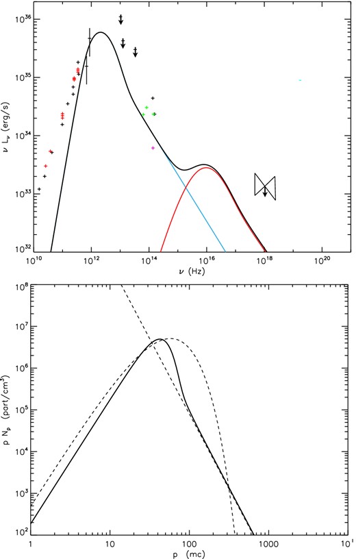
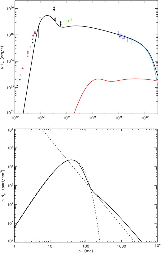
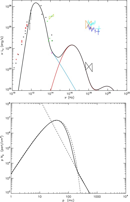
Quiescent spectrum from Sgr A* (top panel) and the associated lepton distribution (bottom panel) in a closed system configuration. On the spectrum, the black data points are taken from Yuan et al. (2003) with the X-ray ‘bowtie’ corresponding to an upper limit for the quiescent state of Sgr A*. The data points on the spectrum are described in details in Section 3.1. The blue curve component of the spectrum corresponds to the synchrotron process, while the red one corresponds to the Compton process. The Bremsstrahlung contribution is not visible in the scale of this plot. On the electron distribution, the solid line is the shape of the calculated distribution from which the spectrum comes from, while the dotted lines indicate a pure Maxwellian plus power-law components for comparison.
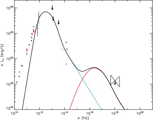
Quiescent spectrum from Sgr A* resulting from the ‘standard’ distribution consisting of a simple Maxwellian plus power law (dotted line in the bottom panel of Fig. 1).
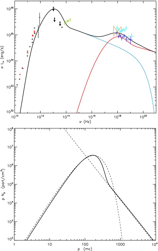
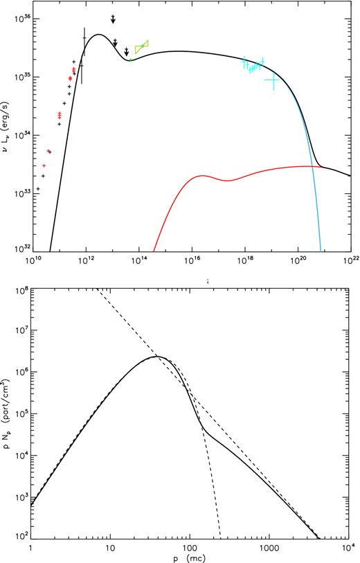
Flare spectrum from Sgr A* (top panel) and the associated lepton distribution (bottom panel) in a closed system configuration. The data points on the spectrum are described in the beginning of Section 3. The blue curve corresponds to the synchrotron process, while the red corresponds to the Compton processes. The Bremsstrahlung contribution is too small to be visible on this scale. On the lepton distribution, the full line corresponds to the actual calculated distribution, while the dotted line is a standard Maxwellian plus power law as a comparison. In all our models (except for Fig. 2), the spectra result from the calculated particle distribution (full line), while the theoretical fixed distribution (dotted line) is just shown as an illustration.
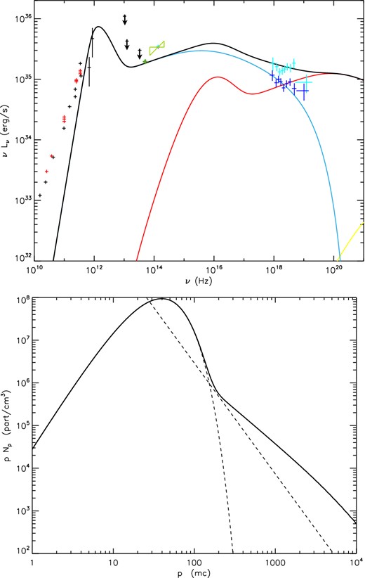
Fig. 4 shows another potential flare model, together with its lepton distribution. This spectrum is similar to Fig. 3 except that the non-thermal synchrotron component is more important than the Compton one. The radius of the emitting region is the same as the density of particles. The magnetic field magnitude is also 48.8 G. The difference comes from the balance between thermal versus non-thermal heating. For this non-thermal synchrotron-dominated spectrum, the non-thermal contribution lnth is more important than previously with a value of 1.9 × 1036 erg s− 1 and a slope of 2.2. The total luminosity is similar to the previous case with L = 4.3 × 1036 erg s− 1.
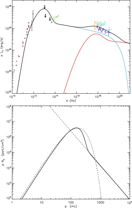
Flare spectrum from Sgr A* (top panel) and the associated lepton distribution (bottom panel) in a closed system configuration. The data points on the spectrum are described in the beginning of Section 3. The blue curve corresponds to the synchrotron processes, while the red corresponds to the Compton processes. It is the same as Fig. 3, but for the case of a dominant synchrotron component with respect to the Compton one. On the electron distribution, the full line is the shape of the actual distribution from which the spectrum comes from, while the dotted lines are pure Maxwellian plus power-law components as a comparison.
2.3.2 The open configuration
3 SGR A* RESULTING SPECTRA
The flare duration varies but the typical time is about 3000 s. The radiative time-scales and the thermalization time are much smaller than the flare duration. The particle and photon distributions are in quasi-steady state at each moment of the flare, and the flare evolution is directly governed by the evolution of model parameters, here namely the acceleration processes described by the parameters lnth and lth. Therefore, we will mostly present and discuss the results from steady-state simulations. That is, we aim at reproducing separately the quiescent and flaring spectra by changing the value of only few parameters. Doing so, we can say that the flaring state is just a transition governed by the increase or decrease of few physical parameters. What is driving these changes is subject to interpretation, but knowing what needs to be modified should give us some good first insight into the physical processes at work.
Table 1 summarizes the characteristics of our different models.
Description of simulations.
| Model | Spectrum | Configuration | B | ne | lth | lnth | linj | s | pesc | ϵk/ϵb | Te | Lbol |
|---|---|---|---|---|---|---|---|---|---|---|---|---|
| (G) | (particles cm− 3) | (×10−5) | (×10−5) | (×10−4) | (×1010 K) | (× 1036erg s− 1) | ||||||
| Fig. 1 | Quiescent | Closed | 154.3 | 4.6 × 10⁶ | 2 | 1 | 0 | 3.60 | 0 | 0.15 | 11.4 | 1.4 |
| Fig. 3 | Flare | Closed | 48.8 | 4.6 × 10⁶ | 7 | 3 | 0 | 2.40 | 0 | 6.32 | 35.0 | 4.8 |
| Fig. 4 | Flare | Closed | 48.8 | 4.6 × 10⁶ | 5 | 4 | 0 | 2.20 | 0 | 5.79 | 33.4 | 4.3 |
| Fig. 5 | Quiescent | Open | 175.3 | 3.3 × 10⁶ | 0 | 1 | 4.64 | 3.60 | 1 | 0.08 | 7.84 | 1.0 |
| Fig. 6 | Flare | Open | 175.3 | 3.3 × 10⁶ | 0 | 9.8 | 4.64 | 2.28 | 1 | 0.09 | 7.90 | 3.8 |
| Fig. 7 | Flare | Open | 175.3 | 3.3 × 10⁶ | 0 | 11.4 | 4.64 | 2.13 | 1 | 0.09 | 7.87 | 4.8 |
| Fig. 8 | Flare | Open | 34.5 | 1.4 × 10⁸ | 0 | 100 | 200 | 2.60 | 1 | 97.16 | 7.79 | 5.8 |
| Fig. 10 | Quiescent | Open | 175.3 | 9.9 × 10⁶ | 0 | 1 | 14 | 3.60 | 1 | 0.24 | 7.86 | 3.8 |
The first column gives the figure number. The second one gives the state of the spectrum we are trying to reproduce (in quiescence or during a flare) and the configuration of the model (closed or open region). B is the magnetic field which is a free input parameter. ne is the density which is also an input parameter in the closed configuration cases (Figs 1, 3, and 4) but an output of the simulations in the other cases. lth is the prescription for thermal heating, and lnth is the prescription for non-thermal heating/acceleration. linj is the injection of particles for the open configuration cases. s is the spectral index used in the non-thermal prescription for acceleration. Pesc gives the probability for particles to escape from the system. ϵk/ϵb is the ratio of kinetic energy over magnetic energy (8π∫mc2(γ − 1)Nγdγ/B2) and is computed after the different models have run. Te is the temperature of the thermal part of the spectrum. Because our lepton distributions are calculated self-consistently, we never have a perfect thermal distribution, but this temperature corresponds to the closest match between the real distribution and the pure Maxwellian (plotted in dotted lines in all our distributions as a comparison), this is of course an output of our models as well. Finally, the last column gives the total luminosity of the spectrum. In the closed configuration case, this luminosity is the direct result of the thermal plus non-thermal compactness parameters, while in the open configuration it results from the balance between injection, escape, and cooling. We remind that in all our models we have R = 2rG, γmin = 50, γmax = 4.6 × 10⁵, and θinj = 13.
3.1 Data
Sgr A*'s spectral energy distribution is made of different observations that are variable and in most cases have not been observed simultaneously in different wavelengths. We have chosen a set of data representative of the overall variation of the spectrum. In all figures, the black radio points are from Falcke et al. (1998) and Zhao (2003), the red radio points are recent ALMA observations from Brinkerink, Falcke et al. in process). The black far-IR upper limits are from Serabyn et al. (1997) and Hornstein et al. (2002), the green MIR data are from Schödel et al. (2011), the pink NIR lower point (in the quiescent spectra) and the cyan NIR upper point (in the flare spectra) are from Ghez et al. (2004), Genzel et al. (2003), and Dodds-Eden et al. (2011). The green ‘bowtie’ is from Bremer et al. (2011) and is one of the few slopes that has been observed so far in the IR. Several flare observations seem to be consistent with this value of the NIR spectral index around −0.6 ± 0.2 (Ghez et al. 2005; Gillessen et al. 2006; Hornstein et al. 2007; Bremer et al. 2011).
The black ‘bowtie’ in the quiescent X-ray is from Baganoff et al. (2001, 2003) and is an upper limit for the central emission because it is contaminated by thermal bremsstrahlung from the outer accreting matter. The orange ‘bowtie’ is a Chandra flare from Nowak et al. (2012). Finally, the blue data points (dark and light blue) are two flares observed with NuSTAR on 2012 July 21 and October 17, respectively (Barrière et al. 2014). Even though the X-ray flares may seem different in shape and slope, they are both acceptably fit by an absorbed power law, and their photon indices are not significantly different (|$2.23^{+0.24}_{-0.22}$| and |$2.04^{+0.22}_{-0.20}$| for the July 21 and October 17 flares, respectively). Barrière et al. 2014, investigated the presence of a cutoff in the October 17 flare, but found that it is not required by the data. The other wiggles in this spectrum (one may see a ‘V’ shape in the low-energy part of the spectrum) are not significant either. One needs to keep in mind that the error bars show the 1σ confidence range, which means that an acceptable fit does not need to go through them all but three out of nine.
Three X-ray flares are shown on the first flaring spectra (Figs 3 and 4), but then we consider only the modelling of one of the NuSTAR flares that extend to higher energies. For a better reproduction of the spectrum, we need to move to the ‘open configuration’ where we present some possible spectra for the July flare or the October flare.
3.2 Sgr A* spectra from a closed region
Fig. 1 shows a spectrum for the quiescent state of Sgr A*, together with the emitting steady-state lepton distribution. For this first spectrum, we consider a density of 4.6 × 10⁶ particles cm−3 (which corresponds to τ = 4 × 10⁻⁶), and we keep this density to study the closed region, i.e. we consider that the number of particles is kept constant in the quiescent and flaring states. In quiescence, the magnetic field is 154.3 G, the plasma is magnetically dominated with ϵk/ϵb = 0.15. The thermal heating is twice the non-thermal one and corresponds to 9.6 × 1035 and 4.8 × 1035 erg s− 1, respectively, so that the total emission reaches 1.4 × 1036 erg s− 1 in quiescence. We can see in the resulting spectrum in Fig. 1 that the non-thermal component is not dominant, and this is not only due to the low value of lnth but also because of the steep injected slope s = 3.6. Nevertheless, this non-thermal component is important in order to reproduce the lower NIR data point. The thermal part contributes mainly to the sub-mm bump. In this case, we can notice how the thermal part of the lepton distribution differs from the standard Maxwellian shape on the bottom panel of Fig. 1. Indeed, for particle energies around p = 102mc, the difference between the calculated distribution and the standard shape in dotted line, can reach almost two orders of magnitude. The steady-state particle distribution is sharper than a pure Maxwellian. Above γ = 100, synchrotron cooling overcomes the anomalous thermalization, and the distribution cuts more sharply than a pure thermal one. This also produces a sharper sub-mm bump as is illustrated in the resulting spectrum (top panel of Fig. 1). In Fig. 2, we plotted the spectral shape resulting from the dotted line of Fig. 1. We can see that the quiescent spectrum would be much wider, reaching the far-IR upper limits. The novelty of our work is illustrated by the difference between Figs 1 and 2, that results from the careful and detailed calculation of the lepton distribution.
Starting from similar conditions as in the quiescent state of Fig. 1, Fig. 3 shows a spectrum for the flaring state of Sgr A*, together with the lepton distribution. The spectrum is dominated by SSC emission (red line), even though the non-thermal synchrotron (blue line) has a non-negligible contribution to the total spectrum. The emitting region is the same as in the quiescent state with the same density of particles. However, the magnetic field has dropped from 154.3 to 48.8 G, the plasma being now kinetically dominated with ϵk/ϵb = 6.3. This dramatic change could be interpreted as being due to magnetic reconnection, a physical process that could be at the origin of the flaring event. When the magnetic field is rearranged, some magnetic energy is converted to kinetic energy, thermal energy, and particle acceleration. In this way, we have a decrease of the magnetic field strength and an increase of the two parameters lth and lnth representing the thermal and non-thermal acceleration, respectively. In this case, to have the Compton dominated spectrum in the flaring state (Fig. 3), the thermal heating increases from 9.6 × 1035 to 3.4 × 1036 erg s− 1, and the non-thermal one from 4.8 × 1035 to 1.4 × 1036 erg s− 1. The non-thermal component has also a much flatter distribution in the flaring state, meaning that the high energies are more populated, while s is steeper during quiescence. With this model, during the flare, the total luminosity reaches 4.8 × 1036 erg s− 1.
The quiescent state is very well reproduced by this closed region configuration model, the sub-mm bump is clearly fitted by synchrotron emission which extends to the lower part of the variable MIR and NIR data, and we are not violating the X-ray limit represented by the black ‘bowtie’. According to the new results from Wang et al. (2013) and Neilsen et al. (2013), saying that the inner region is dominated by non-thermal emission from combined weak flares that can contributes to 10 per cent of the quiescent X-ray, we could be even too low in the X-ray luminosity (lower than 10 per cent of the observed flux). The flaring spectra are somewhat more marginal because the sub-mm contribution is too high compared to two black data points that are upper limits and end up below the spectra. On the other hand, the sub-mm part of the spectrum is also variable on the order of 20 per cent and considering that we do not have perfect simultaneous data, it still provide a close enough interpretation, meaning that we are still within 20 per cent of the actual data point values. In the MIR, the flaring spectra shown in Figs 3 and 4 are in the right range of luminosity, and we can also reproduce the X-ray flare fluxes. The NuSTAR (blue) and Chandra (orange) flare slopes are respected, while the trend of one of the MIR flare (green ‘bowtie’) is not well reproduced at all. We have to keep in mind that our data are not simultaneous and slopes in the MIR have been observed only few times, but still in this case our slope seems to be in contradiction with this observation.
3.3 Plasma with escape and thermal injection
For comparison within the open configuration, we want to reproduce the quiescent spectrum with the assumption that particles flow in and out of the emitting region. Fig. 5 shows such a spectrum, which is similar to the simulated spectrum in Fig. 1. This spectrum is a realistic and acceptable solution for the quiescent state of Sgr A*. The magnetic field magnitude is 175 G with a resulting plasma density of 3.3 × 106 cm−1 that is also magnetically dominated with ϵk/ϵb = 0.08. We note that in this case, the thermal component does not really differ from the pure Maxwellian distribution (see the bottom panel of Fig. 5). Indeed, in this range, radiative cooling is negligible, so that the balance between the thermal particle injection and the uniform particle escape produces a steady-state distribution that is almost the pure Maxwellian. The total luminosity of this spectrum is L = 1.0 × 1036 erg s−1, also equivalent to the previous quiescent fit. From this quiescent spectrum, we next investigate the changes necessary in order to move to the flaring spectrum.

Quiescent spectrum from Sgr A* (top panel) and the associated lepton distribution (bottom panel) with thermal injection and escape (open configuration). The data points are the same as in the previous quiescent spectrum in Fig. 1.
Fig. 6 shows a spectrum for a flaring state of Sgr A*, together with the lepton distribution. The flaring spectrum is dominated by non-thermal synchrotron and reproduce the NuSTAR July flare as well as an IR flare with a slope closer to the usually observed one (flat to slightly rising in the power spectrum). As expected, cooling breaks are observed in the lepton distribution and in the photon spectrum. These are not sharp but span at least one order of magnitude in frequency. The emitting region is the same as in the quiescent state and the magnetic field stays the same as well. The amount of injected particles is the same as in quiescence leading to a constant density. The only change in order to move from the quiescent to the flare spectrum is on the non-thermal component: the heating parameter lnth is increasing by almost one order of magnitude, and the slope becomes flatter (from 3.6 to 2.3 during the flare), meaning that we have more particles in the higher energy part of the electron distribution. So, we must have some physical processes that accelerate the particles more efficiently in the flaring state and create a harder non-thermal distribution. As a consequence the total luminosity increases, reaching 3.8 × 1036 erg s−1.
Flare spectrum from Sgr A* (top panel) and the associated lepton distribution (bottom panel) in the open configuration. The data points are the same as in the previous spectrum in Fig. 3. The electron distribution shows also in dotted line, the pure Maxwellian and power-law curves as a comparison.
We can do the same exercise to reproduce the October NuSTAR flare. This is shown in Fig. 7 for our best case scenario that is really similar to the model on Fig. 6 with non-thermal synchrotron with a cooling break responsible for the flare emission. This is not surprising as we explained earlier in Section 3.1, that both flares are not significantly different and should be modelled with a power-law shape as a fit. As for the July flare, the trigger of the event is on the non-thermal component of the lepton distribution that increases by a bit more than an order of magnitude with a prescribed slope of 2.1, which is a bit flatter than for the July flare. Besides that, the size of the emitting region, the magnetic field, and the density are the same as for the other flare and the same as in quiescence. For the October flare model, we have a slightly higher non-thermal power with a slightly flatter prescription for the acceleration, the total luminosity of this flare spectrum is 4.8 × 1036 erg s−1.
Flare spectrum from Sgr A* (top panel) and the associated lepton distribution (bottom panel) with thermal injection and escape. The data points are the same as in the previous flare spectra on Figs 3, 4, and 6. The calculated electron distribution (full line) and the theoretical one (dotted line) as a comparison.
We investigated an alternative scenario where the X-ray flares would be produced by SSC emission; however, we found that models that account for pure SSC as an emission mechanism have physical parameters that are hardly compatible with what we know of the central region density. Moreover, it leads to a more complex scenario where the large-scale magnetic field and the density of the medium need to be modified during the flare event. Nevertheless, inverse Compton emission could still be a non-negligible component of the overall spectrum, especially at high energies, assuming a weaker magnetic field during the flare and a higher density medium. Fig. 8 gives an illustration of some ‘power-law’ shape X-ray emission that would be a combination of synchrotron and SSC. In this case, the density has increased from 3 × 10⁶ to 1 × 108 cm−1 and the magnetic field has dropped from 175 to 35 G moving to a kinetic dominated flow with ϵk/ϵb = 97.
Flare spectrum from Sgr A* (top panel) and the associated lepton distribution (bottom panel) with thermal injection and escape. The data points are the same as in the previous flare spectra in Figs 3, 4, 6, and 7. The calculated electron distribution (full line) and the theoretical one (dotted line) as a comparison.
We think that the best model for the flaring state of Sgr A* is the one produced by non-thermal synchrotron with a cooling break, as seen on Figs 6 and 7, because the trends of the multiwavelength data are reproduced and only very few parameters need to be adjusted in order to move from the quiescent to the flaring state. This is especially true if we consider that the green ‘bowtie’ is a typical IR slope. The non-thermal synchrotron emission is a simple and elegant solution of the flaring event observed by Chandra and NuSTAR because the overall state of the medium does not change dramatically (for instance the density and magnetic field is kept constant). The acceleration of the electrons leading to the more important and flatter non-thermal lepton distribution is the only modification, and this could be triggered by some plasma instabilities that are not modelled in details here.
Even though magnetic reconnections could also be the initial trigger, it can happen on very small scales and does not necessarily lead to a drop of the global magnetic field magnitude. A possible sudden increase of the density (as in model 8) can be interpreted as an accretion rate fluctuation; however, such fluctuations of more than an order of magnitude are most likely not happening every day in the Galactic Center and would be difficult to interpret. The NuSTAR data being consistent with a power-law shape to higher energies point also in favour of the synchrotron scenarios, as in models 6 and 7.
The sub-mm part of the spectrum is really stable: comparing the quiescent state on Fig. 5 with the sub-mm part of the spectrum on Fig. 6, we have exactly the same contribution around 1012 Hz. This is mainly due to the fact that the magnetic field is kept constant and the injected population is also constant. This configuration gives us in return a constant density. We have to keep in mind that the data are not simultaneous, nevertheless it is an interesting exercise trying to model several wavelength observations in the same time. In the future, simultaneous observations are going to be very important for this kind of multiwavelength study.
We then looked at the time evolution between Figs 5 and 6 to reproduce the X-ray light curve of the July NuSTAR flare. Using our self-consistent calculations, we can also model the time-dependent particle evolution in order to reproduce the flare light curves. This approach has also been considered by Dodds-Eden et al. (2010) in the one zone cell approximation but for a given power-law distribution. The cooling time-scales being very short compared to the flare duration, the time evolution is entirely governed by the physics of the acceleration processes that are not clearly defined. Fig. 9 shows the reproduction of the X-ray light curve between 3 and 79 keV for the same parameter setting as for Figs 5 and 6. During the flare, the non-thermal parameter lnth evolves linearly with time from the quiescent value 10−5 to a maximum value, such that the averaged value over the flare duration is 9.8 × 10⁻⁵ as in our flare spectrum 6. It reaches a maximum value at the peak, and decreases back immediately with a linear dependence. The slope of the accelerated particles is set to 2.28 during the flare event as in our flare spectrum 6, and to 3.60 in quiescence. We note that before the flare event, Sgr A* is not detected by the X-ray satellite NuSTAR because it is too faint, and embedded in the diffuse/unresolved emission, in this case we simply plotted 3σ upper limits.
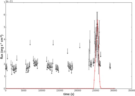
NuSTAR X-ray light curve of the flare event of the 2012 July 21. The black data points are the unabsorbed flux between 3 and 79 keV. When the detection was not strong enough to be significant, we have only plotted upper limits of 3σ (arrows). See Barrière et al. (2014) for the observed light curve. The red curve represents the X-ray light curve from our quiescent spectrum model in Fig. 5 to the flare spectrum model in Fig. 6.
4 CONCLUSION AND OUTLOOK
We are able to reproduce the quiescent spectrum of Sgr A* in two different scenarios: considering that the accretion process is very slow and that the same particles remain a long period of time in the emitting region, and considering that the accretion process is very efficient, with and accretion velocity close to the speed of light; so that particles only remain in the emitting region on short time-scales comparable to the radiative time-scales. To model the flaring state, however, we favour the second scenario that allows a better interpretation of the sub-mm and infrared part of the spectrum. The flaring state spectrum is best reproduced by a plasma that has the same low magnetic field as in quiescent, and the same amount of injected particles. More efficient non-thermal heating processes are responsible for the flaring event, and a flatter non-thermal distribution of electrons is present. Besides this change, all other parameters stay the same when moving from the quiescent to the flaring spectrum (Figs 5 and 6). Our conclusions are in good agreement with Dodds-Eden et al. (2010), who also favoured non-thermal synchrotron processes and a cooling break in order to explain the observed IR and X-ray flares. However, in our study, we do not make the hypothesis of magnetic reconnection as an energy power for the flares, and our conclusions do not favour this particular hypothesis. As in our best case scenario (Figs 5 and 6 or 7), the magnetic field is not required to drop significantly. An important drop in the magnetic field amplitude has also important consequences on the sub-mm and thermal part of the spectrum that we also model here; other parameters have then to be carefully adjusted in order to maintain the sub-mm shape in reasonable values, so we think other acceleration mechanisms are more likely to be happening. Reconnection mechanisms could also occur in very localized regions, and particles would diffuse away from the reconnection sites and radiate in a field which has not reconnected, so we would not notice any significant global drop of the magnetic field amplitude. In our study, we end up with a plasma density of 3.3 × 10⁶ particles cm−3, which is a reasonable value according to observations and theoretical work. But what would happen to the quiescent spectrum (Fig. 1 or 5) if the density increases by a factor of 3 as expected to happen now when the cloud G2 is falling into the Galactic Center? As reported by Gillessen et al. (2012), a dense gas cloud approximately three times the mass of Earth is falling into the accretion zone of Sgr A*, but nothing noticeable has been observed yet from Sgr A*. Fig. 10 represents such a prediction, it has exactly the same settings as the model described on Fig. 5, but the density is three times higher (we have more particle injection). The model predicts a flux increase in the sub-mm bump (1012–1013 Hz), however, the current emission is not well constrained in this band. If the source stays in quiescence, we do not expect a particular increase in the IR, and we have some emission in the ultraviolet due to the first Compton component that is unfortunately not detectable. Even in the X-ray, if the increasing density by a factor of 3 does not trigger a flare event, we do not expect a significant increase from the quiescent X-ray level. Overall, it could well be that we are not detecting any striking changes.
Quiescent spectrum from Sgr A* with the same conditions as in Fig. 5 but assuming an increase of the density by a factor of 3. All the observed data (of quiescent and flaring state) have been kept on the figure. The associated lepton distribution is shown on the bottom panel.
We acknowledge support from The European Community's Seventh Framework Programme (FP7/2007-2013) under grant agreement number ITN 215212 Black Hole Universe. We also acknowledge support from the ‘Nederlandse Onderzoekschool Voor Astronomie’ NOVA Network-3 under NOVA budget number R.2320.0086.
SM and SD gratefully acknowledge support from a Netherlands Organization for Scientific Research (NWO) Vidi Fellowship.
RB and JM acknowledge financial support from both the French National Research Agency (CHAOS project ANR-12-BS05-0009) and the Programme National Hautes Energies.
