


We present a broad-band spectral analysis of the joint XMM–Newton and Nuclear Spectroscopic Telescope Array observational campaign of the narrow-line Seyfert 1 SWIFT J2127.4+5654, consisting of 300 ks performed during three XMM–Newton orbits. We detect a relativistic broadened iron Kα line originating from the innermost regions of the accretion disc surrounding the central black hole, from which we infer an intermediate spin of | $a = 0.58^{+0.11}_{-0.17}$ |. The intrinsic spectrum is steep (Γ = 2.08 ± 0.01) as commonly found in narrow-line Seyfert 1 galaxies, while the cutoff energy (| $E_{\rm c}=108^{+11}_{-10}$ |舁keV) falls within the range observed in broad-line Seyfert 1 galaxies. We measure a low-frequency lag that increases steadily with energy, while at high frequencies, there is a clear lag following the shape of the broad Fe K emission line. Interestingly, the observed Fe K lag in SWIFT J2127.4+5654 is not as broad as in other sources that have maximally spinning black holes. The lag amplitude suggests a continuum-to-reprocessor distance of about 10–20舁rg. These timing results independently support an intermediate black hole spin and a compact corona.
1 INTRODUCTION
According to the commonly accepted paradigm, luminous active galactic nuclei (AGN) are believed to host a supermassive black hole at their centre, surrounded by a geometrically thin accretion disc. The nuclear hard power-law continuum that dominates the spectral emission above 2舁keV is thought to arise in a hot corona above the accretion disc, where UV/optical seed photons from the disc are Compton scattered towards the X-ray band. This primary X-radiation in turn illuminates the disc and it is partly reflected towards the observer's line of sight (two-phase model, Haardt & Maraschi 1991; Haardt, Maraschi & Ghisellini 1994). Such a physical process leads to a power-law spectrum extending to energies determined by the electron temperature in the hot corona. The power-law index is a function of the plasma temperature T and optical depth τ.
The X-ray spectra of unobscured AGN is characterized by ubiquitous and, generally, non-variable features, like the neutral iron Kα narrow core and the Compton reflection component (Perola et al. 2002; Bianchi et al. 2007). These features can be attributed to the reprocessing of the nuclear radiation by distant, neutral matter (i.e. the ‘pc-scale torus’ in the framework of standard Unification Models; Antonucci 1993). Furthermore, there are several important spectral features, like the warm absorber, the soft excess and the relativistic component of the iron Kα line, which are present in a number of objects (Blustin et al. 2005; Crummy et al. 2006); different observations of the same object often show these features to be variable (Piconcelli et al. 2005; Nandra et al. 2007; de La Calle Pérez et al. 2010).
X-ray wavelengths offer the best opportunity in which to investigate the physical properties of the primary nuclear source closest to the event horizon and to give constraints on its geometry. Recent works suggest that most of the emission arises from within ∼20rg (Reis & Miller 2013) and X-ray microlensing experiments confirm that it is compact; in some bright quasars a half-light radius of the corona of rs ≤ 6 rg has been measured (Chartas et al. 2009), where the gravitational radius is defined as rg ≡ GM/c2. Eclipses of the X-ray source have also placed constraints on the size of the hard X-ray emitting region: rs ≤ 30 rg in NGC 1365 (Risaliti et al. 2007; Maiolino et al. 2010; Brenneman et al. 2013), rs ≤ 11 rg in SWIFT J2127.4+5654 (Sanfrutos et al. 2013).
Recently, X-ray reverberation around accreting black holes has also revealed that the corona is compact. On short time-scales, the variability associated with the primary continuum is found to lead the variability associated with the soft excess and the broad iron K spectral features. These time delays are short (e.g. tens of seconds in 1H0707-465, which has a black hole mass of ∼ 2 × 10⁶舁M⊙; Kara et al. 2013a), suggesting that the light travel time between the continuum emitting corona and the reprocessing region is small, within ∼10舁rg. The first detection of X-ray reverberation was found between the continuum and the soft excess (Fabian et al. 2009). In this work, the soft excess was shown to be associated with the broad iron L emission line which peaks at ∼0.8舁keV. Since then, reverberation lags associated with the soft excess and the iron K emission line have been discovered (Zoghbi et al. 2012; De Marco et al. 2013; Kara et al. 2013c), and all reveal that the X-ray emission is coming from very small radii. In this paper, we explore the frequency-dependent time lags in SWIFT J2127.4+5654 that are associated with the soft excess and the broad iron K line.
In addition to these geometric constraints, cutoff energies in several bright Seyfert galaxies have been measured with hard X-ray satellites in the past, such as BeppoSAX (Perola et al. 2002; Dadina 2007) and INTEGRAL (Panessa et al. 2011; de Rosa et al. 2012; Molina et al. 2013). Current measurements of cutoff energies range between 50 and 300舁keV and require spectra extending above 50舁keV for better constraints, due to the contribution from complex spectral components (such as reflection from the accretion disc and from distant material) to the broad-band spectral shape.
Narrow-line Seyfert 1 galaxies (NLS1) are a class of AGN whose spectra show peculiar emission-line and continuum properties. They are considered to be Eddington limit accretors (Boroson & Green 1992) and to systematically host smaller black hole masses than broad-line Seyfert 1 galaxies (Komossa & Xu 2007, and references therein). The primary defining criteria of these objects are the width at half-maximum (FWHM) of the Balmer emission lines in their optical spectra (≲2000舁km舁s−1) and the relative weakness of the [O舁iii] emission at λ5007 (Osterbrock & Pogge 1985). Past X-ray analyses have shown their very variable continua, on time-scales of hours (Ponti et al. 2012). The X-ray spectra of these objects show very steep slopes, between Γ = 2.1 and 2.5 (Boller, Brandt & Fink 1996; Brandt, Fabian & Pounds 1996; Brandt, Mathur & Elvis 1997).
The Nuclear Spectroscopic Telescope Array (NuSTAR; Harrison et al. 2013) is the first high-energy focusing X-ray telescope on orbit, ∼100 times more sensitive in the 10–80舁keV band compared to previous observatories covering these energies, enabling the study of steep spectrum objects at high energies with high precision.
SWIFT J2127.4+5654 (a.k.a. IGR J21277+5656, z = 0.0144) was classified as an NLS1 galaxy on the basis of the observed FWHM of the Hα emission line (∼1180舁km舁s−1; Halpern 2006). It has been first detected with Swift/BAT in the hard X-rays (Tueller et al. 2005). The source was detected in the hard band with INTEGRAL/IBIS and an averaged spectrum was obtained by Malizia et al. (2008) in the 17–100舁keV band by summing the available on-source exposures (and therefore emission states), resulting in a steep spectrum, in the range Γ = 2.4–3. The authors also discussed a single epoch optical spectrum: the NLS1 classification was confirmed and a black hole mass of 1.5 × 10⁷舁M⊙ was inferred. The Swift/XRT data were analysed by the same authors together with the INTEGRAL/IBIS averaged spectrum and the presence of a spectral break or of an exponential cutoff in the range of 30–90舁keV was suggested (Panessa et al. 2011). SWIFT J2127.4+5654 was then observed in 2007 with Suzaku for a total net exposure of 92 ks, a LBol/LEdd ≃ 0.18 and a Γ = 2.06 ± 0.03 were measured (Miniutti et al. 2009). A relativistically broadened Fe Kα emission line was detected, strongly suggesting that SWIFT J2127.4+5654 is powered by accretion on to a rotating Kerr black hole, with an intermediate spin value of a = 0.6 ± 0.2. This result has been also confirmed by Patrick et al. (2011) and in a recent work, using a ∼130 ks long XMM–Newton observation (Sanfrutos et al. 2013). The Fe Kα shape has been also interpreted in terms of reprocessing in a Compton-thick disc-wind (Tatum et al. 2012), which would require super-Eddington luminosities (Reynolds 2012).
We present, in the following, results from a simultaneous NuSTAR and XMM–Newton observational campaign performed in 2012 November. Taking advantage of the unique NuSTAR energy window, we cover the 0.5–80舁keV energy bandwidth. The paper is structured as follows: in Section 2, we discuss the joint NuSTAR and XMM–Newton observations and data reduction, in Sections 3 and 4 we present the spectral and lags analyses, respectively. We discuss and summarize the physical implications of our results in Sections 5 and 6.
2 OBSERVATIONS AND DATA REDUCTION
2.1 NuSTAR
NuSTAR (Harrison et al. 2013) observed SWIFT J2127.4+5654 simultaneously with XMM–Newton with both Focal Plane Module A (FPMA) and B (FPMB) starting on 2012 November 4 for a total of ∼340 ks of elapsed time. The Level 1 data products were processed with the NuSTAR Data Analysis Software (nustardas) package (v. 1.1.1). Cleaned event files (level 2 data products) were produced and calibrated using standard filtering criteria with the NUPIPELINE task and the latest calibration files available in the NuSTAR calibration data base (CALDB). Both extraction radii for the source and background spectra are 1.5舁arcmin. Custom good time intervals files were used to extract the FPMA and FPMB spectra simultaneously with the three XMM–Newton orbits. After this process, the net exposure times for the three observations were 77, 74 and 42 ks, for a total signal-to-noise ratio (SNR) of 215, 235 and 186 for the FPMA, and 209, 234 and 186 for the FPMB, between 3 and 80舁keV. The background-subtracted count rates are 0.631 ± 0.003, 0.798 ± 0.004 and 0.889 ± 0.005 counts舁s−1 for the FPMA, and 0.604 ± 0.003, 0.785 ± 0.003 and 0.876 ± 0.005 counts舁s−1 for the FPMB, between 3 and 80舁keV (Fig. 1).

From the top to the bottom, NuSTAR FPMA+B and XMM–Newton EPIC-Pn light curves in the 3–80舁keV, 2–10舁keV and 0.5–2舁keV energy bands are shown. The ratio between 0.5–2舁keV and 2–10舁keV EPIC-Pn light curves is shown in the bottom panel, straight and dashed lines indicate mean and standard deviation, respectively.
No significant variability is observed in the ratio between the 5–10 and 10–60舁keV count rates (see Fig. 2) during any of the three exposures, suggesting that spectral variability in the NuSTAR bandpass during these observations is only weak.

The ratio between 5–10舁keV and 10–60舁keV NuSTAR FPMA light curves (in 3000舁s bins) is plot versus the time from the start of the NuSTAR pointing, straight and dashed lines indicate mean and standard deviation, respectively.
The three pairs of NuSTAR spectra were binned in order to oversample the instrumental resolution by at least a factor of 2.5 and to have an SNR greater than 3σ in each spectral channel. The cross-calibration constant between the two instruments is consistent with 2 per cent in the three orbits.
2.2 XMM–Newton
SWIFT J2127.4+5654 was observed by XMM–Newton (Jansen et al. 2001) for ∼300 ks, starting on 2012 November 4, during three consecutive revolutions (OBSID 0693781701, 0693781801 and 0693781901) with the EPIC CCD cameras, the Pn (Strüder et al. 2001) and the two MOS (Turner et al. 2001), operated in small window and medium filter mode. Data from the MOS detectors are not included in our analysis since they suffered strongly from photon pileup. The extraction radii and the optimal time cuts for flaring particle background were computed with sas 12 (Gabriel et al. 2004) via an iterative process which leads to a maximization of the SNR, similar to the approach described in Piconcelli et al. (2004). The resulting optimal extraction radius is 40舁arcsec and the background spectra were extracted from source-free circular regions with a radius of about 50舁arcsec.
After this process, the net exposure times were 94, 94 and 50 ks for the EPIC-Pn, with 0.5–10舁keV count rates of 5.411 ± 0.007, 6.498 ± 0.008 and 7.787 ± 0.013 counts舁s−1 for the three orbits (Fig. 1), respectively. The observation naturally divides into low-, medium- and high-flux states. The 2–10舁keV flux of the source during the third orbit (high-flux state) is consistent with the one observed by Suzaku in 2007 (Miniutti et al. 2009). Spectra were binned in order to oversample the instrumental resolution by at least a factor of 3 and to have no less than 30 counts in each background-subtracted spectral channel. This allows the applicability of χ2 statistics. We do not include the 1.8–2.5舁keV energy band due to calibration effects associated with the Si/Au edge (Smith, Guainazzi & Marinucci 2013).
3 SPECTRAL ANALYSIS
The adopted cosmological parameters are H0 = 70舁km舁s−1舁Mpc−1, | $\Omega _\Lambda = 0.73$ | and Ωm = 0.27, i.e. the default ones in xspec 12.8.1 (Arnaud 1996). Errors correspond to the 90 per cent confidence level for one interesting parameter (Δχ2 = 2.7), if not stated otherwise.
We started our analysis fitting the medium-flux state spectrum with a power law absorbed with only the Galactic column density (7.65 × 10²¹舁cm−2; Kalberla et al. 2005) between 2–4 and 7.5–10舁keV. In Fig. 3, the broad-band data-to-model ratio is shown (the continuum is modelled with a Γ = 1.89 power law), and both a broad iron Kα line and a strong Compton hump are clearly visible.
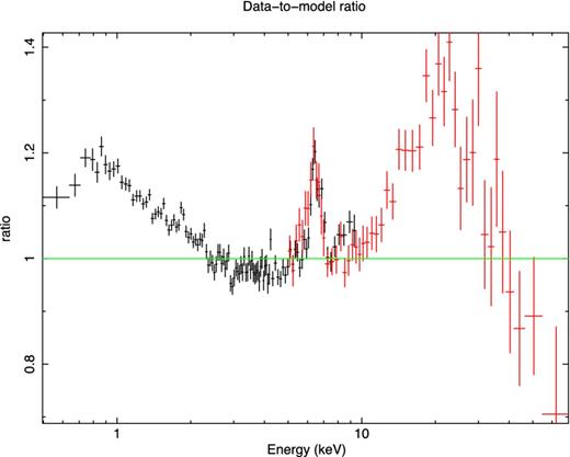
Data-to-model ratio of the medium flux state (Orbit 2). EPIC-Pn and FPMA spectra are shown in black and red, respectively. The continuum is modelled with a Γ = 1.9 power law (fitted between 2–4舁keV and 7.5–10舁keV).
3.1 EPIC PN spectral analysis
A phenomenological fit is applied in the 3–10舁keV range to the three spectra, with a baseline model composed by a power law and four Gaussian lines, to reproduce the broad and narrow components of the Fe Kα emission line and the Fe舁xxv Kα, Fe舁xxvi Kα lines at 6.7 and 6.966舁keV, respectively. We left the normalization of the power law free to vary between the three orbits to include intrinsic flux variations of the source. The fit is good (χ2/dof = 331/321 = 1.03) and no strong residuals are present; results are presented in Table 1. Comparing the 2013 observation with the old Suzaku one, it is interesting noting that the broad component of the iron line (| $\sigma = 0.22^{+0.23}_{-0.12}$ |舁keV) is less prominent and the EW of the narrow Fe Kα in the last orbit (the one comparable in flux with the Suzaku observation) is consistent with the one reported in Miniutti et al. (2009).
Best-fitting parameters for the 3–10舁keV XMM phenomenological fit. Asterisks indicate fixed values, energies are in keV units, fluxes in 10−5 ph cm−2舁s−1 units and equivalent widths for the three orbits are in eV units.
| Id. | Energy | Flux | EW1 | EW2 | EW3 |
|---|---|---|---|---|---|
| Fe Kα [Br.] | | $6.37^{+0.22}_{-0.12}$ | | | $1.3^{+1.4}_{-0.7}$ | | | $53^{+55}_{-25}$ | | | $43^{+45}_{-21}$ | | | $38^{+40}_{-18}$ | |
| Fe Kα [Nar.] | | $6.46^{+0.03}_{-0.06}$ | | | $0.8^{+0.4}_{-0.4}$ | | | $31^{+15}_{-15}$ | | | $27^{+13}_{-13}$ | | | $23^{+12}_{-12}$ | |
| Fe xxv Kα | 6.7* | | $0.5^{+0.3}_{-0.3}$ | | | $20^{+10}_{-10}$ | | | $17^{+8}_{-8}$ | | | $15^{+7}_{-7}$ | |
| Fe舁xxvi Kα | 6.966* | | $0.6^{+0.2}_{-0.4}$ | | | $28^{+6}_{-10}$ | | | $24^{+5}_{-8}$ | | | $21^{+4}_{-7}$ | |
We then simultaneously fitted the 0.5–10舁keV EPIC-Pn spectra from the three orbits with a more physical model, leaving the normalizations of the primary power law and of the disc reflection component free to vary, to take into account the flux variations of the source. When we use a model composed of an absorbed power law and cold distant reflection the fit is not good (χ2/dof = 849/457 = 1.86) and strong residuals around the iron Kα band are present.
We then added a relativistically blurred reflection component arising from an ionized accretion disc and a further absorber at the distance of the source (Sanfrutos et al. 2013). We used xillver for both cold and ionized reflection (García et al. 2013) and relconv for relativistic smearing (Dauser et al. 2013). The inclusion of a blurred reflection component in the model greatly improves the fit (χ2/dof = 507/451 = 1.12). The addition of two emission lines at 6.7舁keV (Fe xxv Kα, actually a triplet) and at 6.966舁keV (Fe舁xxvi Kα), with fluxes consistent with the ones reported in Table 1, marginally improves the fit χ2/dof = 498/449 = 1.11. Replacing the intrinsic neutral absorber with an ionized one, we find an upper limit to the ionization state of log舁ξ ≤ −0.54, leading to no improvement of the fit. The photon index of the primary continuum is steep (Γ = 2.11 ± 0.01), as commonly found for NLS1 galaxies and no strong residuals are present throughout the energy band, with the exception of a feature in the spectrum from the third orbit around ∼0.8舁keV which is not attributable to any known spectral feature (Fig. 4). The excess in the soft energy band, shown in Fig. 3, is a combination of the steep primary continuum and the blurred ionized reflection, no additional components to the model described above are needed. We find an intermediate value for the black hole spin (a = 0.5 ± 0.2), in good agreement with the value measured by Suzaku, values for the emissivity and inclination of the disc are also consistent with previous analyses (Miniutti et al. 2009). Best-fitting parameters are presented in Table 2. When we leave the column density of the neutral local absorber and the photon indices of the primary continua free to vary between the three spectra, a marginal improvement of the fit (χ2/dof = 481/445 = 1.07) is found, with no variations from combined best-fitting parameters.

EPIC-Pn 0.5–10舁keV best fit and residuals with a model where blurred relativistic reflection is taken into account, no structured residuals are seen.
Best-fitting parameters for reflection and absorption models. Column densities are in 1021舁cm−2 units, disc inclination angles are in degrees, ionization parameters ξ are in erg cm s−1 units, Fe abundance is with respect to the solar value and cutoff energy Ec is in keV units. Power-law normalizations are in ph cm−2舁s−1舁keV−1 at 1舁keV and q is the adimensional parameter for the disc emissivity. The subscript p indicates that the parameter pegged at its minimal allowed value.
| XMM | XMM+NuSTAR | |
|---|---|---|
| NH | 2.2 ± 0.1 | 2.13 ± 0.05 |
| Γ | 2.11 ± 0.01 | | $2.08^{+0.01}_{-0.01}$ | |
| | $E\rm _c$ | | – | | $108^{+11}_{-10}$ | |
| | $N_{\rm pow}^1$ | (×10−3) | 9.6 ± 0.1 | 9.6 ± 0.1 |
| | $N_{\rm pow}^2$ | | 11.4 ± 0.1 | 11.4 ± 0.1 |
| | $N_{\rm pow}^3$ | | 14.1 ± 0.1 | 13.9 ± 0.1 |
| Nneutral (×10−4) | 1.25 ± 0.25 | 0.95 ± 0.15 |
| q | | $6.1^{+2.1}_{-1.7}$ | | | $6.3^{+1.1}_{-1.0}$ | |
| a | 0.5 ± 0.2 | | $0.58^{+0.11}_{-0.17}$ | |
| i | | $48^{+5}_{-3}$ | | 49 ± 2 |
| ξ | <20 | <8 |
| AFe | | $0.54^{+0.06}_{-0.04p}$ | | | $0.71^{+0.05}_{-0.05}$ | |
| | $N_{\rm refl}^1$ | (×10−4) | 2.9 ± 0.5 | 2.7 ± 0.3 |
| | $N_{\rm refl}^2$ | | 3.7 ± 0.5 | 3.5 ± 0.3 |
| | $N_{\rm refl}^3$ | | 3.0 ± 0.5 | 3.0 ± 0.4 |
| χ2/dof | 498/449 = 1.11 | 1733/1566 = 1.10 |
3.2 Broad-band spectral analysis
We then included the six 3–80舁keV NuSTAR (FPMA and FPMB) spectra in our analysis, extending the spectral coverage up to 80舁keV. We left the cross-calibration constants between XMM and NuSTAR free to vary. A photon index of Γ = 2.08 ± 0.01 is found, in agreement with previous Suzaku observations (Miniutti et al. 2009). We get a best fit χ2/dof = 1907/1567 = 1.21 and strong, structured residuals can be seen above ∼20舁keV (Fig. 5, left-hand panel), suggesting the presence of a high energy cutoff.
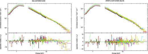
Left-hand panel: broad-band fit of the NuSTAR and XMM spectra with a model that does not take into account the high energy cutoff. Clear residuals can be seen above ∼20舁keV. Right-hand panel: broad-band XMM +NuSTAR best fit when a cutoff energy is properly modelled.
Therefore, we substituted the primary power law with the cutoffpl model in xspec and tied the values of the cutoff energies to the ones of the reflection components.1 The fit greatly improves (Δχ2 = 174, for one additional degree of freedom), a χ2/dof = 1733/1566 = 1.11 is found and no strong residuals are present in the whole energy band (Fig. 5, right-hand panel). Best-fitting parameters can be found in Table 2 and fluxes, luminosities and Eddington ratios in Table 3. The cross-calibration factors between the Pn and the FPMA, FPMB detectors are KFPMA = 1.045 ± 0.007 and KFPMB = 1.074 ± 0.007. We measure a cutoff energy | $E_{\rm c} = 108^{+11}_{-10}$ |舁keV and Γ = 2.08 ± 0.01: Fig. 6 (left-hand panel) presents the contour plot of photon index versus cutoff energy.
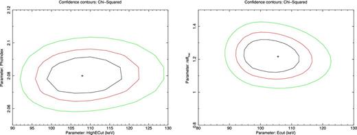
Δχ2 = 2.30, 6.17 and 11.83 contours (corresponding approximately to 68, 95 and 99.7 per cent confidence levels) for the cutoff energy Ec and photon index Γ (left-hand panel) and for the cutoff energy and the blurred ionized reflection fraction in the second orbit (right-hand panel).
Best-fitting fluxes and luminosities in different energy intervals. Fluxes are in 10−11舁erg cm−2舁s−1 units and are observed. Luminosities are in 1043舁erg舁s−1 units and are corrected for absorption. We calculated Lbol from the 2–10舁keV luminosity, applying the relation of Marconi et al. (2004) for the bolometric corrections (this factor is also consistent with the lowest bolometric correction for this accretion rate presented in Vasudevan & Fabian 2009). A value for the black hole mass of 1.5 × 10⁷ M⊙ has been used (Malizia et al. 2008).
| Orb. 1 | Orb. 2 | Orb. 3 | |
|---|---|---|---|
| F2-10舁keV | 2.40 ± 0.02 | 2.87 ± 0.02 | 3.32 ± 0.02 |
| L2-10舁keV | 1.13 ± 0.01 | 1.35 ± 0.05 | 1.57 ± 0.05 |
| | $L_{\rm 3-80\ keV}^{\rm pow}$ | | 1.61 ± 0.02 | 1.92 ± 0.02 | 2.35 ± 0.02 |
| F20-100舁keV | 2.67 ± 0.03 | 3.21 ± 0.03 | 3.34 ± 0.03 |
| L20-100舁keV | 1.25 ± 0.01 | 1.50 ± 0.05 | 1.57 ± 0.05 |
| Lbol/LEdd | ≃0.11 | ≃0.14 | ≃0.16 |
In order to estimate the relative strength of the Compton hump (arising from both distant and blurred ionized reflection components) with respect to the primary continuum, we followed a method similar to the one described in Walton et al. (2013) for NGC 1365, using the relative normalizations of the reflection (modelled with pexrav, with the inclination angle and iron abundance fixed to best-fitting values) and of the power-law components, above 10舁keV. We find values of R1 = 1.5 ± 0.2, R2 = 1.6 ± 0.2 and R3 = 1.1 ± 0.2 for the three sets of spectra, respectively.
Thanks to the NuSTAR+XMM broad-band view, the degeneracy between the contribution from the ionized and the cold reflector can be broken, using recent X-ray disc reflection models that include relativistic blurring and a direct measure of R. We substituted the blurred ionized reflection and primary components in the broad-band best-fitting model for relxill (a model that includes both relativistic effects and reflection from an accretion disc, Garcia et al. 2014). The reflection fraction R has been left to vary between the three orbits. The overall fit is good (χ2/dof = 1756/1570 = 1.11) and no differences from best-fitting parameters presented in Table 2 are found. The contribution of the blurred reflection component from the disc to the total reflection fraction in the three orbits is | $R_1^{\rm disc} = 1.1\pm 0.1$ |, | $R_2^{\rm disc} = 1.2\pm 0.1$ | and | $R_3^{\rm disc} = 0.9\pm 0.1$ |. The contour plot of the cutoff energy Ec and the | $R_2^{\rm disc}$ | parameter is shown in Fig. 6, right-hand panel. If we consider a lamp-post geometry and use relxilllp (with spin and inclination parameters fixed to their best-fitting values) we find a height of the X-ray source of 25 ± 10舁rg, consistent with the estimates discussed in Section 5.
Once a best fit is obtained we try to reproduce the primary continuum (modelled with cutoffpl in xspec so far) with a more physical model where the electron energy (kTe) and the coronal optical depth (τ) can be disentangled, using different geometries. Photon index and cutoff energy are fixed to their best-fitting values in the reflection components. We use the comptt model in xspec (Titarchuk 1994), which assumes that the corona is distributed either in a slab or a spherical geometry. In such a model, the soft photon input spectrum is a Wien law; we fixed the temperature to 50舁eV, appropriate for MBH ≈ 107舁M⊙. In the case of a slab geometry, the fit is good (χ2/dof =1733/1569 = 1.10) and best-fitting values of | $kT_{\rm e} = 68^{+37}_{-32}$ |舁keV and | $\tau = 0.35^{+0.35}_{-0.19}$ | are found. When a spherical corona is considered, we find a statistically equivalent fit (χ2/dof = 1734/1569 = 1.10) and best-fitting values are | $kT_{\rm e} = 53_{-26}^{+28}$ |舁keV and | $\tau = 1.35_{-0.67}^{+1.03}$ |. In both geometries, no significant variations from the best-fitting values in Table 2 are found and 3–80舁keV fluxes of the primary continuum are consistent with the ones presented in Table 3. As already pointed out in Brenneman et al. (2014) in the case of IC 4329A, the difference in optical depth when two different geometries are taken into account is primarily due to the different meaning of this parameter in the two geometries: the optical depth for a slab geometry is taken vertically, while that for a sphere is taken radially (see Titarchuk 1994, for a more detailed description of the models).
4 XMM–NEWTON LAGS
Finally, in addition to this broad-band spectral analysis, we looked for time lags using the XMM–Newton observations. The lags were computed using the standard Fourier technique, described in Nowak et al. (1999), where the phase lag is found between the Fourier transform of two light curves. The phase lag is converted into a frequency-dependent time lag by dividing by 2πf, where f is the temporal frequency.
We start in usual way by looking for lags associated with the soft excess (as in Fabian et al. 2009; De Marco et al. 2013). The left-hand panel of Fig. 7 shows the frequency-dependent lag between 0.3–1 and 1–5舁keV. A positive lag indicates a time delay in the hard band, which we find at frequencies below 3.5 × 10⁻⁵舁Hz. The lag goes to zero above this frequency. We then probe the frequency-dependent lag between 3–5 and 5–8舁keV, where there is less obscuration (right-hand panel of Fig. 7). This shows the hard 5–8舁keV band lagging at higher frequencies, as well (at ν < 30 × 10−5舁Hz).
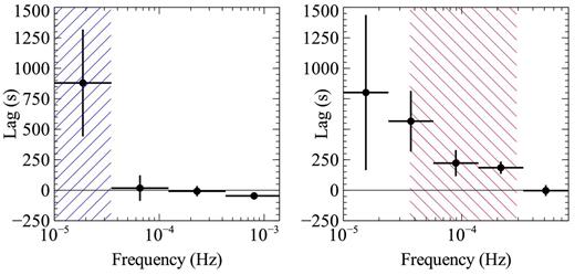
To investigate further, we compute the ‘lag-energy spectrum’, to find the average time delays associated with the energy spectrum. The zero-point of the lag is dictated by the chosen reference band (for this analysis, it was the entire 0.3–10舁keV, excluding the band of interest), and so it is the relative lag between energy bins that is meaningful. The left-hand panel of Fig. 8 shows the lag-energy spectrum for frequencies less than 3.5 × 10⁻⁵舁Hz (where we found the 1–5舁keV band lagging behind the 0.3–1舁keV band). The time delay increases steadily with energy, without any obvious spectral features, similar to the low-frequency lag-energy spectra in several other AGN (Kara et al. 2013b; Walton et al. 2013b). We then probe higher frequencies,in the range ν = [3.5–30] × 10− 5Hz, where the 5–8舁keV band lags the 3–5舁keV band (right-hand panel of Fig. 8). The high-frequency lag-energy spectrum shows little to no lag between the soft excess and the 1–5舁keV band, but then jumps up 200舁s at ∼5舁keV. The lag peaks at 6–8舁keV, and the points from 5–8舁keV are >4σ above the continuum lag. It does not show the obvious decrease above 8舁keV that is often seen in high-frequency lag-energy spectra, but statistics are low at this high-frequency, so we cannot rule out a downturn of the lag at the highest energies.
5 DISCUSSION
We analysed the NuSTAR+XMM spectrum of the NLS1 galaxy SWIFT J2127.4+5654. A relativistic reflection component is found in proximity of an intermediate spin Kerr black hole (| $a = 0.58^{+0.11}_{-0.17}$ |), confirming past Suzaku results (Miniutti et al. 2009; Patrick et al. 2011) and providing a very accurate measurement of the intermediate black hole spin of this source, thanks to the broad (0.5–80舁keV) spectral coverage. Fig. 9 shows the different components of the model, including the primary continuum, the relativistic blurred reflection of the disc and the emission from distant, neutral matter. The contribution from the blurred ionized reflection arising from the accretion disc to the total reflection fraction has been measured and it is described in Section 3.2. The values obtained are similar to those estimated for other type 1 AGN in Walton et al. (2013a). Fig. 10 shows the goodness-of-fit as a function of the black hole spin: the broader spectral coverage with respect to past analyses allows us to rule out a maximally spinning black hole with a significance >5σ, and a non-rotating Schwarzschild black hole (a = 0) is rejected with a significance >3σ. We find that the accretion disc parameters (disc emissivity and inclination angle) are in agreement with the ones discussed in the past and the steep emissivity (ϵ ∝ r−6.3) suggests that the Fe emission arises from the innermost regions of the disc (see Miniutti & Fabian 2004, for a more detailed description of the light bending model). Other physical interpretations have been recently discussed for the joint XMM and Suzaku analysis of Fairall 9 (Lohfink et al. 2012). The intermediate black hole spin we measure carries information about the accretion history of the source, and a value of 0.6–0.7 suggests a scenario where the black hole mass in SWIFT J2127.4+5654 is due to a recent black hole merger (see Volonteri et al. 2005; Berti & Volonteri 2008, for a detailed discussion of the different cases) and Volonteri, Sikora & Lasota (2007) for a description of the morphology dependent spin evolution.
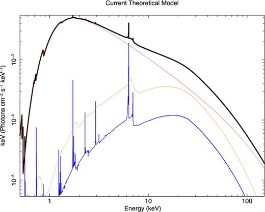
Relativistic reflection model between 0.5 and 150舁keV. Different components such as the relativistic blurred ionized reflection (in orange), the primary continuum (in red) and neutral reflection from distant material (in blue) can be clearly seen.
The high data quality above 10舁keV, thanks to the unique NuSTAR spectral coverage, permits us to measure a cutoff energy | $E_{\rm c} = 108^{+11}_{-10}$ |舁keV with unprecedented accuracy, marginally consistent with prior INTEGRAL results where a cutoff energy of | $49^{+49}_{-17}$ |舁keV (Panessa et al. 2011) was measured. Using a Comptonization model to reproduce the spectral shape of the primary continuum, we find values of | $kT_{\rm e} = 68^{+37}_{-32}$ |舁keV and | $\tau = 0.35^{+0.35}_{-0.19}$ | with a slab geometry and | $kT_{\rm e} = 53_{-26}^{+28}$ |舁keV and | $\tau = 1.35_{-0.67}^{+1.03}$ | with a spherical geometry. The power-law continuum is an estimate of the power dissipated in the corona, and it is ∼57 per cent of the total 3–80舁keV luminosity (L3 − 80舁keVpow = 1.92 × 1043舁erg舁s−1 for the second orbit, Table 3). This represents ∼7.5 per cent of the bolometric luminosity of the source (Lbol ∼ 2.6 × 1044舁erg舁s−1).
The electron plasma temperatures agree with the ones found in Brenneman et al. (2014) for the broad-line Seyfert 1 galaxy (BLSy1) IC 4329A, but the lower values for τ in SWIFT J2127.4+5654 suggest a different geometry in the corona. Indeed, NLS1 galaxies are high rate accreting objects with low black hole masses (Bian & Zhao 2004; McLure & Jarvis 2004; Netzer & Trakhtenbrot 2007). The lower optical depth might indeed explain why the relativistic reflection in this object (∼33 per cent of the total 3–80舁keV luminosity) is more prominent than in IC 4329A, where the power-law continuum component is higher, being ∼87 per cent of the total 5–79舁keV luminosity.
SWIFT J2127.4+5654 shows significant lags over a wide range of frequencies. X-ray time lags are largely agreed to be caused by two separate processes: by the light travel time between the X-ray source and the ionized accretion disc and by mass accretion rate fluctuations that get propagated inwards on the viscous time-scale and cause the soft coronal emission from large radii to respond before the harder coronal emission at smaller radii. When we measure the lag at a particular frequency, we are measuring the average time lag, and so if both effects are contributing to the lag at a particular frequency, it can be difficult to disentangle which process is responsible for the lag. In sources with a large soft excess that is dominated by relativistically blurred emission likes (i.e. 1H0707-495 and IRAS 13224-3809), we can easily disentangle these two effects by looking at the lag between ∼0.3–1 and ∼1–4舁keV. In these sources, we find that at low frequencies, the hard band lags the soft (due to dominating propagation lags) and at high frequencies, the soft band lags the hard (due to greater reverberation between corona and accretion disc). For SWIFT J2127.4+5654, the 0.3–1 to 1–5舁keV frequency-dependent lag shows the typical hard lag of ∼1000舁s at frequencies below 3.5 × 10⁻⁵舁Hz (left-hand panel of Fig. 7). It does not show an obvious soft reverberation lag, and this likely because the soft excess is not very strong, due to absorption or because of low iron abundance. However, we can look for reverberation signatures at higher energies, where the Fe K line is strong, and there is little absorption. The frequency-dependent lag in the right-hand panel of Fig. 7 shows the 5–8舁keV lagging behind the 3–5舁keV band up to higher frequencies of ∼3 × 10⁻⁴舁Hz. While some of this lag is likely due to propagation effects (i.e. below 3.5 × 10⁻⁵舁Hz), the high-frequency lag (3.5-30 × 10− 5舁Hz) is likely caused by reverberation, where the emission from the Fe K line centroid (5–8舁keV) lags behind the continuum or red wing of the line (3–5舁keV). The lag-energy spectra support this hypothesis (Fig. 8). The low-frequency lag-energy spectrum below 3.5 × 10⁻⁵舁Hz shows a nearly featureless spectrum, increasing with energy (indicative of intrinsic propagation lags in the corona), while in the higher frequencies (ν = [3.5–30] × 10−5舁Hz), we see a different shape. There is still a little contribution from the soft excess, but we see a large increase in lag at 5舁keV, also where we see the red wing of the Fe K line. The lag does not decrease above 8舁keV, as is often seen in Fe K reverberation lags, and this could be an effect of the inclination of the disc (Cackett et al. 2014), or just too low statistics to confirm a decrease in the lag.
Left-hand panel: the frequency-dependent lag between 0.3–1 and 1–5舁keV. A positive lag indicates that the hard band lags behind the soft band. We see a hard lag at ν < 3.5 × 10⁻⁵舁Hz, and zero lag above that frequency. Poisson noise begins to dominate the power spectrum at ν ∼ 5 × 10⁻⁴舁Hz. (The blue hash shows the frequency range explored for the lag-energy spectrum in the left-hand panel of Fig. 8.) Right-hand panel: the frequency-dependent lag between the 3–5 and 5–8舁keV bands. The hard lag extends up to 3 × 10⁻⁴舁Hz. (The red hash shows the frequency range for the lag-energy spectrum in the right-hand panel of Fig. 8.)
![Left-hand panel: the lag-energy spectrum for low frequencies, ν < 3.5 × 10⁻⁵舁Hz (corresponding to the frequency range shown in blue hash in Fig. 7. The lag increases steadily with energy. Right-hand panel: the lag-energy spectrum for frequencies ν = [3.5–30] × 10−5舁Hz (the red hash in the right-hand panel of Fig. 7. This shows little lag between the continuum and soft excess, and a sharp increase in the lag at >5舁keV.](https://oup.silverchair-cdn.com/oup/backfile/Content_public/Journal/mnras/440/3/10.1093_mnras_stu404/3/m_stu404fig8.jpeg?Expires=1750254641&Signature=gXjxrznqbfGyACMZc5VDIOBMDbFBEMBhJlHtZ7yJlc~m~Lz~OLZwLWdQjMXtT36YPDxe3Gn~OZag~1hxTsiza5OA4cepjVp6UvKCauyYgxzuLN8IR4K1HU3FwKp2BI-lDGWoDZMdVg4GVcDmysH48~4EcGqKm9dAlMuhc6Ac~vlua3ju8Kjk0aqPhx-cVWA5kz4ofo4QQCpXnEq3qUuROrzpG5ZExXLijBNBJ6WizPwsAUj5yQ08xQnuk1mt6mtHhIxicttVDAUNdfG8Tb4nVTy0SMrp60oB9BwEofTsSMO-Zn1DpYFmW38I3sxrQk0lrEs35Fh42IyNHiBmg0nf6w__&Key-Pair-Id=APKAIE5G5CRDK6RD3PGA)
Left-hand panel: the lag-energy spectrum for low frequencies, ν < 3.5 × 10⁻⁵舁Hz (corresponding to the frequency range shown in blue hash in Fig. 7. The lag increases steadily with energy. Right-hand panel: the lag-energy spectrum for frequencies ν = [3.5–30] × 10−5舁Hz (the red hash in the right-hand panel of Fig. 7. This shows little lag between the continuum and soft excess, and a sharp increase in the lag at >5舁keV.
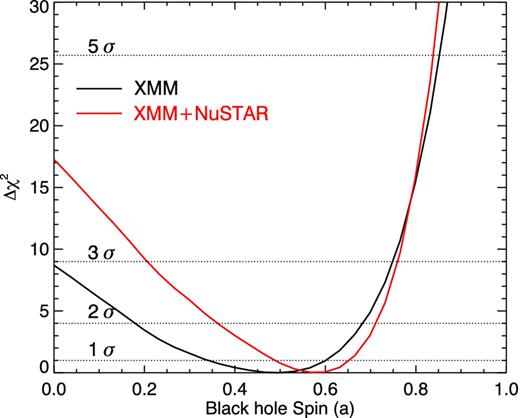
Goodness-of-fit variation as a function of the black hole spin. Dashed, horizontal lines indicate Δχ2 values of 1, 4, 9 and 25.7 which correspond approximately to 1, 2, 3 and 5σ confidence levels.
In principle, the amplitude of the lag reflects the light travel time between the primary X-ray source and the accretion disc, and can give an estimate of the size of the corona (Wilkins & Fabian 2013). However, it is important to take dilution into account before converting the time delay to a physical distance. For example, at 6.5舁keV, the ionized reflection component contributes to ∼30 per cent of the entire variable emission (i.e. not including the cold reflection component), while the continuum contributes to remaining 70 per cent. Therefore, the intrinsic lag will be diluted by 70 per cent, since 70 per cent of the emission comes from the direct continuum. Furthermore, the reference band to which we measure the lag at each energy is also affected by dilution. It is composed of roughly 10 per cent reflection and 90 per cent power law. If the intrinsic lag in SWIFT J2127.4+5654 is 1000舁s, then, including all the effects of dilution, the observed lag at 6.5舁keV is ∼ 200舁s (which is close to what we observe). Given the lower reflection fraction at soft energies below 1舁keV, the observed lag should be closer to 50舁s, which is also consistent with what we see in the right-hand panel of Fig. 8. Assuming an intrinsic lag of 1000舁s puts the X-ray source at a height of ∼13舁rg above the disc, for a black hole mass of 1.5 × 10⁷舁M⊙ (Malizia et al. 2008).
The high-frequency lag-energy spectrum (ν = [3.5–30] × 10−5舁Hz) shows that the Fe K lag profile is not very broad. Importantly, this timing result is independent of the spectral results, which also shows the emission line is not broad. All other sources with Fe K reverberation lags have a maximally spinning black hole, and show Fe K reverberation lags as low as 3–4舁keV. This source only shows a reverberation lag at above 5舁keV, as expected for a larger inner radius. This is very strong evidence for an intermediate black hole spin.
6 SUMMARY
We presented a NuSTAR+XMM broad-band (0.5–80舁keV) spectral analysis of the joint observational campaign in 2012 of SWIFT J2127.4+5654.
The main results of this paper can be summarized as follows.
Thanks to the broader spectral coverage with respect to past analyses, a relativistic reflection component is found in proximity of an intermediate spin Kerr black hole (| $a = 0.58^{+0.11}_{-0.17}$ |), a maximally spinning black hole can be ruled out with a significance >5σ and a non-rotating Schwarzschild black hole is rejected with a significance >3σ;
The high data quality above 10舁keV allowed us to measure a cutoff energy | $E_{\rm c} = 108^{+11}_{-10}$ |舁keV with unprecedented precision;
The high-frequency lag-energy spectrum shows an Fe K reverberation lag. Unlike other maximally spinning black holes that have broad Fe K lags, SWIFT J2127.4+5654 has a narrower lag profile, which independently suggests an intermediate spin black hole.
We thank the referee for her/his comments and suggestions that greatly improved the paper. AM thanks Javier Garcia and Thomas Dauser for the efforts in producing xillver and relxill tables to use in this paper. AM and GM acknowledge financial support from Italian Space Agency under grant ASI/INAF I/037/12/0-011/13 and from the European Union Seventh Framework Programme (FP7/2007-2013) under grant agreement no. 312789. PA and FB acknowledge support from Basal-CATA PFB-06/2007 (FEB), CONICYT-Chile FONDECYT 1101024 (FEB) and Anillo ACT1101 (FEB, PA). MB acknowledges support from the International Fulbright Science and Technology Award. This work was supported under NASA Contract no. NNG08FD60C, and made use of data from the NuSTAR mission, a project led by the California Institute of Technology, managed by the Jet Propulsion Laboratory, and funded by the National Aeronautics and Space Administration. We thank the NuSTAR Operations, Software and Calibration teams for support with the execution and analysis of these observations. This research has made use of the NuSTAR Data Analysis Software (nustardas) jointly developed by the ASI Science Data Center (ASDC, Italy) and the California Institute of Technology (USA).
A test version of xillver has been used, where the cutoff energy is a variable parameter.
REFERENCES
