


Abstract
Numerous upcoming observations, such as Wide-Field Infrared Survey Telescope, Baryon Oscillation Spectroscopic Survey (BOSS), BigBOSS, Large Synoptic Survey Telescope, Euclid and Planck, will constrain dark energy (DE)'s equation of state with great precision. They may well find that the ratio of pressure to energy density, w, is −1, meaning DE is equivalent to a cosmological constant. However, many time-varying DE models have also been proposed. A single parametrization to test a broad class of them and that is itself motivated by a physical picture is therefore desirable. We suggest that the simplest model of DE has the same mechanism as inflation, likely a scalar field slowly rolling down its potential. If this is so, DE will have a generic equation of state and the Universe will have a generic dependence of the Hubble constant on redshift, independent of the potential's starting value and shape. This equation of state and expression for the Hubble constant offer the desired model-independent but physically motivated parametrization, because they will hold for most of the standard scalar field models of DE such as quintessence and phantom DE. Up until now two-parameter descriptions of w have been available, but this work finds an additional approximation that leads to a single-parameter model. Using it, we conduct a χ2 analysis and find that experiments in the next seven years should be able to distinguish any of these time-varying DE models on the one hand from a cosmological constant on the other to 73 per cent confidence if w today differs from −1 by 3.5 per cent. In the limit of perfectly accurate measurements of Ωm and H0, this confidence would rise to 96 per cent. We also include discussion of the current status of DE experiments, a table compiling the techniques each will use and tables of the precisions of the experiments for which this information was available at the time of publication.
INTRODUCTION
The Universe is now undergoing an accelerated expansion of space itself, driven by dark energy (DE), a negative pressure component that constitutes 73 per cent of the current energy density (Perlmutter et al. 1998; Perlmutter, Turner & White 1999; Riess et al. 1998; Komatsu et al. 2011). While there is much evidence for DE's existence, we at present lack insight into its essence. Observational efforts have focused on measuring its equation of state, parametrized by w ≡ p/ρ = pressure/energy density, in the hope that so doing will offer understanding of DE's essential nature.
Faced with a proliferation of theoretical models, observers have used parametrizations, such as that of Chevallier–Polarski–Linder, w = w0 + wa(1 − a), where a is the scalefactor, to assess proposed programmes (e.g. Chevallier & Polarski 2001; Linder 2003; Albrecht et al. 2006; for model compendia, see Copeland, Sami & Tsujikawa 2006; Li, Li & Zhang 2011). These parametrizations are supposed to allow a wide variety of models to be tested, since models can produce predictions for e.g. w0 and wa. However, these parametrizations also build in a shape for w(a), one not based on any physical model. Therefore, it may be dangerous to design experiments and analyse results to look for these shapes, which there is no particular reason to believe w(a) for DE in fact has. But what is the alternative? While there is no shortage of models, there is one of funding, time and resources.
Ockham's razor would suggest that, all else being equal, the simplest model is the best. The simplest model, in our view, would take advantage of the fact that we have already most likely seen one epoch of accelerated expansion: inflation in the early universe (Guth 1981, 2007; Guth & Kaiser 2005). The idea that DE now is produced by the same mechanism as inflation then is simple – and it immediately suggests that certain DE models are implausible.1
There are a variety of models for inflation, but a popular, simple class of models that seems to fit all observational constraints has inflation being driven by a scalar field in slow-roll (SR; Albrecht & Steinhardt 1982; Linde 1982). Indeed, values of the scalar spectral tilt ns less than unity are a hallmark of SR inflation that is in fact observed (Linde 2002; Komatsu et al. 2011). In a previous paper (Gott & Slepian 2011), we focused on a specific SR inflationary (and, by analogy, DE) model: the quadratic potential associated with Linde's chaotic inflation. This model for inflation is observationally allowed, and has the potential to be confirmed in the near future if Planck detects the tensor mode amplitude r the model predicts (for Planck details, see Planck: the scientific programme 2005; Geisbuesch & Hobson 2007; de Putter, Zahn & Linder 2009).
Nonetheless, at present, while SR itself is a compelling and broadly accepted model for inflation, the details of the shape of the potential and starting value of the scalar field are unknown; this is also the case for phantom DE, to which we show that our results apply. Consequently, in this paper, we simplify and generalize our previous work (Gott & Slepian 2011) by exploring the observational signature of DE as a scalar field slowly rolling down its potential.2 We find the generic result that if DE is a scalar field in SR, w + 1 evolves with redshift proportionally to 1/H2, with w the ratio of pressure to energy density in the DE and H the Hubble constant (also shown in Gott & Slepian 2011). This result is independent of the initial value and shape of the potential as long as the SR conditions are met (see Section 2.1). We apply this scaling to find a closed-form approximate formula for the Hubble constant in an SR DE cosmology. This makes it easy to find the luminosity and angular diameter distances and chart their differences from those for a w ≡ −1 cosmology. These differences have a characteristic shape: the observational signature of SR DE.
The paper is laid out as follows. In the remainder of this introduction, we offer a brief overview of pervious work on parametrizing and constraining scalar field models of DE similar to those discussed here. In Section 2, we derive formulae for the DE equation of state and the Hubble constant if DE is a scalar field slowly rolling down its potential, and show that, in addition to quintessence, these formulae apply to phantom DE. In Section 3, we review common techniques for observing DE, and in Section 4 turn to current and future experiments. Section 5 outlines our method for determining the confidence with which SR DE (be it quintessence or phantom) may be distinguished from a cosmological constant, carrying out a χ2 analysis first neglecting errors in the cosmological parameters and then accounting for them. Section 6 presents and discusses the results of this latter calculation, while Section 7 concludes by placing our work in context and recapitulating the paper's central points.
Appendix A presents discussion of the self-consistency and accuracy of the approximations of Section 2 and some illustrative numerical results from the exact solution of the field equation of motion (EOM) and the Friedmann equation for typical potentials in the DE models we consider. We also provide low-redshift expressions for the fractional differences in Hubble constant and comoving distance between SR and cosmological constant cosmologies, scalings for the χ2's we will have earlier (Section 5) computed numerically, and finally, the method we will have used to reconstruct the coefficients of the confidence ellipse presented in Section 6. Appendix B comprises tables of the experimental precisions of Wide-Field Infrared Survey Telescope (WFIRST), Big Baryon Oscillation Spectroscopic Survey (BigBOSS), Euclid, Large Synoptic Survey Telescope (LSST) and Baryon Oscillation Spectroscopic Survey (BOSS) as used in Section 5.
The central points of the paper are as follows.
If DE is not equivalent to a cosmological constant, then we suggest that it is likely a scalar field in SR by analogy with inflation. Even if it phantom DE:
It will have a generic equation of state given by equation (9) and a generic H(z) given by equation (14).
With this generic H(z), observations in the next seven years can in principle distinguish between these forms of time-varying DE on the one hand and a cosmological constant on the other.3
Neglecting errors in the cosmological parameters and taking the difference from w = −1 at present to be 3.5 per cent, this can be done to 96 per cent confidence. The confidence levels of a possible detection neglecting errors for other values of w today are illustrated in Fig. 4.
For w + 1 = 3.5 per cent today and accounting for the possibility of errors in the cosmological parameters, SR DE may be distinguished from cosmological constant DE with 73 per cent confidence. The confidence levels of a possible detection for other values of w today are illustrated in Fig. 11.
Previous parametrizations and constraints for SR DE
Numerous authors have worked to develop parametrizations of SR DE, as well as used observations to place constraints on these models. Here we provide a brief review of work closely bearing on our own; for a more extensive treatment, see Chiba, De Felice & Tsujikawa (2013), Chiba et al. (2009) and Gott & Slepian (2011). Dutta & Scherrer (2008) provided an expansion for a scalar field with w ≈ −1 rolling near a local maximum in its potential. This extended earlier work by Scherrer & Sen (2008) by generalizing to potentials with non-zero curvature. Crittenden, Majerotto & Piazza (2007), Neupane & Scherer (2008) and Cahn, de Putter & Linder (2008) offered other early attempts to develop both appropriate SR conditions and parametrizations for w. Chiba (2009) represents a continuation of these efforts, deriving general SR conditions which allow a two-parameter form for w that further generalizes the results of Dutta & Scherrer (2008).4 Both Chiba (2009) and Dutta & Scherrer (2008) make the point that SR DE models are in general poorly described by the Chevallier–Polarski–Linder parametrization w(z) = w0 + wa(1 − a), a comment we emphasize again here.
Overall, then, on the theory side, previous work had succeeded in reducing SR quintessence models to an equation of state w described by two parameters. The main advance of this work is to further collapse this representation to a one-parameter class of models. Previous work required an additional parameter because it effectively described the value of the acceleration in the EOM or, equivalently, the curvature of the potential. This was deemed necessary because, in contrast with the inflationary case, the acceleration cannot always be taken to be small. However, in this work we show that as long as the acceleration is either small or roughly constant in time, it will not affect the scaling of w with time, meaning it can be eliminated from the problem. This argument is made in a physically intuitive way in Section 2, and we take a more mathematically rigorous approach, as well as quantifying the error introduced by this approximation in Appendix A. Fig. A8 in particular shows that the error our approximation introduces should be at least an order of magnitude lower than the signal we expect to use to distinguish SR DE from a cosmological constant for the representative case of V ∝ ϕ2. We also obtain more general analytic expressions for this error which suggest that this should hold for other potentials.
We now turn to a brief review of prior work placing observational constraints on parametrizations of SR DE. The most comprehensive work to date is Chiba et al. (2013), which puts bounds on the parameters for w using Type Ia supernovae (SNe Ia), the cosmic microwave background (CMB) and the baryon acoustic oscillation (BAO). For thawing models (models where the field has begun to evolve only at late times; see Caldwell & Linder 2005), they use Chiba's (2009) two-parameter model, while for tracking freezing models [where the field has now frozen to a halt and different initial conditions converge to a common trajectory (tracker) (Chiba et al. 2013)], they use the two-parameter form of Chiba (2009). For scaling freezing models (the equation of state scales with the background fluid's), numerical simulations are employed. Previously, Dutta & Scherrer (2008) and Chiba et al. (2009) had done this analysis for thawing models with smaller data sets, while Chiba (2010) and Wang, Chen & Chen (2012) did similarly for tracking freezing models. Novosyadlyj, Sergijenko & Apunevych (2011) do such an analysis using a two-parameter model developed in Novosyadlyj et al. (2010). Since our formula for w has one rather than two parameters, these results unfortunately do not give much insight into the most likely values of δw0 = w + 1 if w follows the formula we obtain. In future we hope to use the data sets available to do a similar analysis to constrain this formula.
SR SCALAR FIELD DE
Equation of state
We begin by defining δw = w + 1: simply the difference between w and negative one, a worthwhile subject of attention because it would be interesting if observation finds w ≠ −1 (or δw ≠ 0). We currently know that w ≈ −1 to an accuracy of approximately 7 per cent (Komatsu et al. 2011). If future observations tighten the limits around w = −1, that will increase confidence in the standard cosmological constant model, but will not tell us anything new about DE.
The most exciting result of future observations would be to find a value of w ≠ −1; for then we would learn something new about DE. Of all the models of DE with w ≠ −1, we would argue that SR DE is the most conservative, since we have seen that behaviour in the Universe before during inflation.
If one hopes to detect a significant deviation of w from −1, it is helpful to know the functional form w(z) is likely to take. That will be our goal here.
In what follows, when discussing the scalar field and its potential, we will work in Planck units, c = ℏ = 8πG = 1.
Evidently, small δw at present implies |$\dot{\phi }^2 \ll V$| at present. To connect this with the traditional analysis of an SR field in inflation, note that the condition |$\dot{\phi } \ll V$| (which is implied by the above) is just the first of the two SR conditions usually imposed (see e.g. Lesgourgues 2006). In inflationary cosmology, this condition comes from the need for a roughly constant energy density to drive exponential expansion. Since this energy density is offered by the scalar field's potential, that potential has to be nearly constant, and so |$\dot{\phi }$| must be small compared to V(ϕ). The same applies for DE, as we observe exponential expansion today. Furthermore, we know that w is not very much different from −1 for DE now, so if DE is a scalar field, then to be observationally allowed, δw must be small now. Thus, we must have |$\dot{\phi }^2 \ll V$| now.
Note the analogy of equation (4) to that for a ball rolling down a hill with a frictional force. In such a situation, the ball quickly reaches the terminal velocity and |$\ddot{\phi }$| becomes small. With this in mind, it should be intuitively clear why in SR inflationary models |$\ddot{\phi }$| is small (see e.g. Lyth & Liddle 2000; Copeland et al. 2006). This is traditionally the second of the two SR conditions imposed in inflationary cosmology, and, in that context, is needed to guarantee that the first (|$\dot{\phi }^2 \ll V$|) holds in general and not just at one particular time (Lesgourgues 2006).
If the scaling were an equality, this would duplicate the standard result in inflationary cosmology (see e.g. Lesgourgues 2006).
In summary, then, for small δw, SR applies, |$\dot{\phi }$| is small and |$\delta w\propto \dot{\phi }^{2}.$| When the field reaches the terminal velocity, the acceleration |$\ddot{\phi }$| is nearly zero, so the Hubble friction term |$3H\dot{\phi }$| is balanced by the slope of the potential the field is rolling down, − ∂V/∂ϕ. This is analogous to a ball rolling down a hill: it will reach the terminal velocity when energy dissipation from friction cancels out the energy it gains by moving to lower values of its potential. Finally, if |$\dot{\phi }$| is small, ϕ is roughly constant in time, so ∂V/∂ϕ will be roughly constant as well. This means |$\dot{\phi }\propto H^{-1}$|, which leads to equation (9). This derivation is valid for any smooth scalar field potential for δw sufficiently small compared to unity.
Note finally that the field we have considered above is essentially a quintessence model of DE. For a review of recent work on quintessence DE, see e.g. De Boni et al. (2011) and references therein or Novosyadlyj et al. (2010).
Hubble constant
Application to phantom DE
Phantom DE, also often referred to as ‘ghost’ DE, has negative kinetic energy and leads to an equation of state w ≥ −1 for the kinetic energy-dominated phase and w ≤ −1 for the potential energy-dominated phase. These models reach a ‘big rip’ singularity where the energy density becomes infinite in finite proper time; see Li et al. (2011) and Caldwell (2002) for further discussion, and Cline, Jeon & Moore (2004) for criticisms. For an example of a simple, minimal model of a phantom field, with non-canonical kinetic terms but no potential, see Chiba, Okabe & Yamaguchi (2000). For observational constraints on phantom DE models, see Novosyadlyj et al. (2012) and for forecasts of the possibility that future observations will distinguish between phantom DE and quintessence see Novosyadlyj et al. (2013).
TECHNIQUES FOR OBSERVING DE
Since many proposed experiments (e.g. WFIRST, Euclid, Planck) will use multiple methods to study DE, in this section we briefly review the physics and status of the main techniques, moving in the next to a discussion of specific experiments. For an up-to-date and extremely comprehensive review, see Weinberg et al. (2013); here our treatment will seek simply to provide basics sufficient to outline available tests for the theoretical results we have thus far developed.
BAO
BAO are one of the most promising ways to measure the expansion history of the universe (both the angular diameter distance dA and the Hubble constant H) and hence w for DE. Eisenstein et al. initially detected the BAO signature in 2005 with measurements of luminous red galaxies (LRGs) in Sloan Digital Sky Survey (SDSS-III) data, and since then the precision of this technique has significantly increased (Eisenstein et al. 2005; Seo & Eisenstein 2007).
The major challenge for BAO measurements is non-linear structure formation, which smears out the peak in the galaxy–galaxy pair correlation function by jostling galaxies by 3-10 Mpc. Fortunately, since this effect is random and not systematic, it only leads to a systematic error of the order of 0.5 per cent which can be corrected for with the help of large N-body simulations. Further, the effects of non-linear growth are not severe because the BAO scale has only gone mildly non-linear by now (Eisenstein, Seo & White 2007; Eisenstein et al. 2011). For further discussion, see Padmanabhan & White (2009), Noh, White & Padmanabhan (2009) and Ivezic et al. (2011).
Supernovae
SN measurements have several sources of error. In order from the source to us, they are evolution of SNe with cosmological time, dust in SNe's host galaxies, gravitational lensing, intersection with Earth's atmosphere (not a problem for space-based telescopes), the telescope itself, the filters, the detector response and, finally, the interpretation of the data (Perlmutter 2011). For further discussion, see Ivezic et al. (2011); here, we touch briefly on dust and interpretation of data, as both are areas of recent progress.
Dust absorbs and scatters SNe Ia more in the blue than the red, and makes it difficult to tell their intrinsic brightness. Recent work by Chotard et al. (2011) improves correction by using silicon (Si) and calcium (Ca) features to derive a dust-reddening law. They find a reddening law compatible with a Cardelli extinction law. This is a useful result because Cardelli extinction is well understood, as it is what applies locally in the interstellar medium (Cardelli, Clayton & Mathis 1989).
Interpretation of data is complicated by the fact that SNe are not all exactly the same. To make them better standard candles, ‘stretch correction’ is applied. In 1992, Phillips observed that there is a correlation between the intrinsic brightness at maximum light and the duration of the light curve for SNe Ia (Phillips 1993; Li et al. 2011). This has been used to reduce the 1σ spread in peak B-band luminosity from 0.3 to 0.10–0.15 mag (Kim 2004). Once this is done, further standardization is achieved by, at a given redshift, averaging over many SNe and then comparing to an average over many SNe at another, different redshift. More precise would be to compare SNe that have exactly the same spectral features at different redshifts one-on-one. Efforts to do higher precision distance measurements using these so-called SN twins are just beginning, but with promising results. So far, of 59 SNe studied, 15 twins have been found. It is hoped that there are not many intrinsically different subtypes of SNe Ia, and hence that many twins will be found out of the SNe for which spectra are already available (Perlmutter 2011).
We conclude by briefly noting what data sets are available for SNe. The largest and latest (2010) data set, Union2, has 557 SNe Ia (Li et al. 2011; Perlmutter 2011). Other earlier samples include Union (307 SNe Ia, 2008) and Constitution (added an additional 90 low-z SNe to Union, 2009).
CMB, weak lensing, clusters and topology
The temperature anisotropies in the CMB are affected by DE, and so measuring them constrains it. The relative temperature anisotropies δT/T are expanded in terms of the spherical harmonics Ylm, and the power spectrum is therefore plotted as a function of the wavenumber l. Hence, the amplitude of the power spectrum at a given l corresponds to the anisotropy on that angular scale. DE alters the angular diameter distance dA and thereby changes the angular scale (and so the wavenumber) at which a given anisotropy occurs. See Copeland et al. (2006) and Melchiorri et al. (2003) for further detail. DE also alters the CMB through the integrated Sachs–Wolfe (ISW) effect, a redshift that occurs when the gravitational potential Φ is time dependent. For Ωm < 1, Φ varies with time, leading to an ISW effect that is particularly strong for large-scale power (l ≲ 20) (Copeland et al. 2006).
Finally, the low-l modes of the CMB are most sensitive to DE, as they have most recently re-entered the causal horizon, and it is only at z ≲ 2 that DE became dominant. Zinn (2012) shows that different values of the equation of state, specifically modelled as that of SR DE, will shift the amplitudes of the modes with l ≲ 200 (see Fig. 1). This is an additional avenue for CMB measurements to constrain the equation of state, especially expected to be fruitful because Planck should soon provide cosmic-variance-limited measurements of these low-l modes. Unfortunately, as Fig. 2 illustrates, Zinn finds that the low-l modes of the CMB do not provide a very strong constraint at all on δw0. For further discussion of the method, see Zinn (2012).
Weak lensing (WL) is the distortion of the images of distant galaxies as the light we observe from them is bent by intervening matter. First found in the 1990s around individual haloes, and detected in 2000 due to large-scale structure (LSS), WL is a probe of the matter distribution and hence plays the role of DE in the growth of structure. Lensing can create distortions in shape, size and brightness; most easily measurable are distortions in shape, termed ‘cosmic shear’, which are ≃1 per cent. Because typical intrinsic differences in galaxy shapes are ≃30–40 per cent, a large sample of galaxies must be averaged over to detect WL. For further discussion, see Li et al. (2011), Ivezic et al. (2011, and references therein) and Heavens (2009).
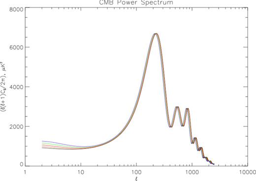
Shift in amplitudes of low-l modes for different values of δw0 ≡ w0 + 1. Black, orange and red correspond to phantom DE with values of δw0 = −0.385, −0.105 and −0.086, respectively; green and blue correspond to scalar field DE with δw0 = 0.173 and 0.453. The high-l modes are shifted from right to left due simply to the effect of SR DE on dA(z = 1089).

A 95 per cent confidence ellipsoid showing the constraint low-l CMB measurements offer between H0 (in km s−1 Mpc−1) (vertical axis), Ωm (left-hand axis) and δw0 (rightmost axis).
Lensing is also used to detect galaxy clusters (CL), which in turn can be counted as a function of mass and redshift and compared with simulation to shed light on DE's role in cosmological expansion. CL can also be detected via optical and infrared imaging and spectroscopy, X-ray imaging and spectroscopy, and the Sunyaev–Zel'dovich (SZ) effect. For further discussion, see Li et al. (2011) and sources therein.
Additional constraints on DE can come from the topology of the LSS, for instance as measured using LRGs in SDSS-III (Gott et al. 2009). It is hoped that topology will provide independent measures of w with about three-fifths the accuracy of the BAO method. Genus topology counts features in the cosmic web and thereby measures rs (Park & Kim 2010). The genus (number of doughnut holes minus number of isolated voids or CL) per unit smoothing length cubed tells the physical scale because the genus depends only on the smoothed power spectrum at recombination. The latter depends directly on rs and can be measured from the CMB. Adopting smoothing lengths ls = (16, 24, 34 h− 1 Mpc), the genus as a function of volume fraction may be calculated as in Gott et al. (2009). The genus per smoothing length cubed in each case provides the ratio ls/rs, with rs the BAO scale as in equation (20).
The topology technique makes it possible to make an independent estimate of, for instance, dA(z = 0.6)/rs [and therefore of dA(z = 0.6)] to an accuracy of 1.7 per cent using BOSS (Park et al. 2012; Speare 2012). This estimate is independent of the estimate of dA(z = 0.6) made by the BAO method because that method is using scales of 144 Mpc to fit the baryon oscillation features in the power spectrum while the topology method uses smoothing scales of 16–34 h−1 Mpc (which are also in the linear regime) to effectively fit the entire power spectrum. Park & Kim (2010) have shown using N-body simulations that the genus measurement is particularly unaffected by non-linear and biasing effects. The median density contour, which is what primarily determines the genus, does not change much as long as the smoothing length ls is large enough to put one into the linear regime. This condition is met by the proposed smoothing lengths for LRGs. If, for instance, the topology technique is used in addition to BAO and the errors are combined in quadrature, BOSS can measure e.g. dA(z = 0.6) to an accuracy of 0.9 per cent.
CURRENT AND UPCOMING OBSERVATIONS
Numerous DE experiments are either in progress or upcoming in the next decade. We treat the missions in two sections: those that have already at least begun physical construction and those that have not. We summarize all the missions we discuss (starting date and techniques) in Table 1.
Current and upcoming surveys: starting date and techniques used. Note that DES and LSST will yield H(z) from the BAO, while BOSS, eBOSS and BigBOSS will yield both H(z) and dA (Blanton, personal communication).
| Survey | Year | SNe | WL | CL | BAO |
|---|---|---|---|---|---|
| HST | Ongoing | X | X | X | – |
| CFHTLS | Fin. 2009 | X | X | – | – |
| BOSS | Begun | – | – | – | X |
| SPT | First results | – | – | X | – |
| Planck | First results | – | – | X | – |
| PanSTARRS | Begun | – | X | X | – |
| LAMOST | Begun | ? | ? | ? | X |
| DES | 2012 | X | X | X | X |
| HETDEX | 2012 | – | – | – | X |
| BigBOSS | 2017 | – | – | – | X |
| eBOSS | 2014 | – | – | – | X |
| Euclid | 2017 | – | X | – | X |
| WFIRST | 2020 | X | X | – | X |
| LSST | 2020 | X | X | – | X |
| SKA | 2020 | – | X | X | X |
| ALPACA | ? | X | X | X | – |
Current
The Hubble Space Telescope (HST) made SN measurements critical to confirming DE's existence, and it is still active in DE measurements, continuing its SN work as well as being first to use the lensing around a galaxy CL (Abell 1689) for DE (HST website7). The Canada–France–Hawaii Legacy Survey (CFHTLS), which ran from 2003 to 2009 and has one data release still remaining, used SNe, via a deep survey to detect and monitor ∼500 SNe Ia, and WL, via a wide survey over 170 square degrees. It also made galaxy distribution measurements (using a wide survey) likely to be useful for topology (CFHTLS website8). In 2009, the Panoramic Survey Telescope and Rapid Response System (Pan-STARRS) began observing with its prototype single-mirror telescope; it will constrain DE via SNe, WL and CL (Pan-STARRS website9). Also using CL, detected via the SZ effect, the South Pole Telescope (SPT) will survey 4000 square degrees and has already claimed the first use of CL for cosmology (SPT website10; Vanderlinde et al. 2010).
Planck, launched in 2009 and already reporting data, will use both CMB and CL to constrain DE. For further details, see Planck: the scientific programme (2005), Geisbuesch & Hobson (2007) and de Putter et al. (2009).
The most significant near-term project using BAO is the BOSS. Running from 2008 to 2014, it will measure 1.5 million LRGs to z = .8. This will constitute a seven-fold improvement on the LSS data from SDSS-II: this comes from, first, a factor of 2 improvement in the instrument and, second, the fact that BOSS will focus on the LSS using more luminous galaxies that can be traced to larger distances (Eisenstein et al. 2011). The next survey to use BAO will be the Large Sky Area Multi-Object Fiber Spectroscopic Telescope (LAMOST), a ground-based wide-field optical telescope on which construction was finished in 2008. Though limited by the small number of clear nights at its location in China (Hebei Province), it will produce the most accurate map to date of the baryons and dark matter in the Milky Way, constraining both DE and the growth of structure (LAMOST website11); Day 2010).
Dark Energy Survey (DES), begun in late 2011, is one of the few surveys to use SNe, WL, CL and BAO. Since SNe and BAO measure the expansion rate, while WL and CL also measure the growth of structure, cross-comparison of these results can test not only DE but general relativity (DES website12). Hobby–Eberly Telescope Dark Energy Experiment (HETDEX), using the existing Hobby–Eberly Telescope at McDonald Observatory (Davis Mountains, Texas), began in 2012 January and is doing a 3 yr redshift survey of nearly one million galaxies to measure BAO (HETDEX website13).
Upcoming
The BigBOSS, expected to begin surveying in 2017, will use LRGs to z = 1.0 and bright O ii emission line galaxies out to z = 1.7 (20 million in total) to measure BAO to 0.4 per cent for 0.5 < z < 1.0 and to 0.6 per cent for 1 < z < 1.7 (BigBOSS website). Euclid (after the Greek geometer) is a satellite of the European Space Agency with launch planned for 2017. It will measure both WL and BAO, covering approximately half the sky in a 20 000 square degree survey; it will also have a 40 square degree deep survey mode (Euclid website14; Refregier et al. 2010).
The WFIRST is a planned United States effort for 2020, though its funding prospects are uncertain. It will use SNe, WL and BAO, and should provide strong constraints on DE (Green et al. 2012; WFIRST website). Ultimately, the WFIRST mission goals may be accomplished using one of two HST-sized telescopes donated to NASA by the Department of Defense. The LSST, currently in the design and development and ‘private construction’ phase, will use SNe, WL and BAO, obtaining sub-per cent precision in H(z) and per cent precision on the angular diameter distance at 10 logarithmically spaced redshifts (LSST website; Ivezic et al. 2011). Square Kilometer Array (SKA) is an Australian effort to build a very long baseline radio telescope array; in early 2012 it was decided that the telescope will have sites in South Africa, Australia and New Zealand. It will survey a billion galaxies out to z ≃ 1.5, allowing the use of the WL, CL and BAO techniques (Blake et al. 2005). Finally, Advanced Liquid-mirror Probe for Astrophysics, Cosmology, and Asteroids (ALPACA) will use SNe, WL and CL, finding 50 000 SNe Ia per year to z ∼ 0.8 and 70 000 galaxy CL (ALPACA website15). Efforts to gain funding for ALPACA are still active and a paper updating the science case is expected in 2013 (Crotts, personal communication).
METHOD
Observational signature
We first compute the angular diameter distance dA and the luminosity distance dL for a cosmological constant cosmology by numerically evaluating equations (A24), (A25) and (A27) (see Appendix A3) using the Hubble constant as a function of redshift for a flat cosmology with negligible radiation and cosmological constant DE. Note again that this will only be valid for z ≪ 3196, but since no observations take place at nearly such a high redshift, this is not a problematic restriction. We then compute dA and dL for an SR DE cosmology by numerically evaluating the same equations (A24, A25 and A27) but now using the Hubble constant in an SR cosmology, given by equation (14), rather than the Hubble constant in a cosmological constant cosmology. We finally compute the fractional difference in luminosity and angular diameter distance between the SR model and the cosmological constant model, ΔdL/dL, −1 = ΔdA/dA, −1 = Δdc/dc, −1 via equation (A26), where the final equality involves the comoving distance (see Appendix A3 for proof). ΔdL ≡ dL, SR − dL, −1, with dL, SR the luminosity distance in a slow-roll cosmology and dL, −1 that for a cosmological constant cosmology. Analogous definitions are made for ΔdA, dA, SR, dA, −1, and Δdc and dc, −1.
Our results are displayed in Fig. 3 – they are the observational signature of SR DE. This figure shows that the best z to observe to see a difference between the two cosmologies in dA is z ≃ 1, notably, roughly where SN searches are indeed able to measure dA. The best z to observe to see how the cosmologies differ in H is z ≃ 0.5 – roughly where e.g. BOSS and BigBoss will look. The blue curve (for ΔdA/dA, −1) begins at zero because ΔdA, 0/dA, −1, 0 = 0 = ΔdL, 0/dL, −1, 0 today – there is no difference between the SR and cosmological constant cosmologies today because we normalize each to the same (current best) value of H0 (thus far, we are neglecting errors in the cosmological parameters). As z increases, DE influences H(z), causing it to differ between SR and cosmological constant cosmologies, and hence causing a difference in dc between the two. This difference in dc is nearly monotonic in z for small z because dc stems from an integral over z; hence, the slight difference at each redshift between the two cosmologies accumulates as one looks farther back into the past.
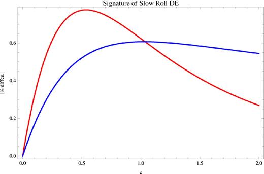
The blue curve shows the magnitude of the per cent difference in comoving distance (which is the same as the per cent difference for luminosity distance or angular diameter distance; see Appendix A3) between SR and cosmological constant cosmologies as a function of redshift z. We have plotted the magnitude because Δdc/dc, −1 is negative: the comoving distance in an SR cosmology is lower than that for a cosmological constant cosmology. This is because an SR cosmology will have expanded faster in the past than a cosmological constant cosmology, as equation (23) shows. Of course, the χ2 analysis we later carry out is insensitive to the sign of Δdc/dc, −1. The red curve shows the per cent difference in the Hubble constant between the two cosmologies. Our calculations are for δw0 = 3.5 per cent as that is roughly consistent with the current best value of w0 from WMAP+BAO+H0. The difference curves are zero today because we impose that the Hubble constant today has the same value in each model. The differences increase as we integrate back in time over z and pick up the difference in the SR versus cosmological constant equations of state. The differences then turn around and move back towards zero because for z ≳ 1 DE is subdominant to matter and so the importance of a difference between cosmologies in the DE sector fades.
However, at z ≃ 1.5, DE begins to be subdominant to matter, and since the two cosmologies being compared do not differ in the matter sector, the fractional difference in comoving distance between the two, Δdc/dc, −1, begins to drop as the effects of DE become less and less important while the denominator dc continues to grow. Note that the difference between the SR DE cosmology's comoving distance and the cosmological constant cosmology's comoving distance is negative because the comoving distance is the physical distance with cosmological expansion ‘taken out’. As equation (23) shows, an SR DE cosmology will have expanded more in the past than a cosmological constant cosmology, so more expansion gets ‘taken out’ to compute the comoving distance and hence the comoving distance in an SR DE cosmology is lower than that in a cosmological constant cosmology.
Now, we turn to the red curve, describing the fractional difference in the Hubble constant, ΔH/H− 1 ≡ (HSR − H− 1)/H− 1, with all quantities defined analogously to those for dL. ΔH/H−1 also begins at zero, again because we have normalized both cosmologies to have the correct value of H0 today (thus far, we are neglecting errors in the cosmological parameters). It is monotonic in z up to z ≃ 0.5; this is simply because the Hubble constant grows with increasing z, and for an SR cosmology, the DE term will also have a z-dependence (see equation 14). Hence, the fractional difference between an SR and a cosmological constant cosmology will grow with z as long as DE is dominant.
Just as with the curve for Δdc/dc, −1, the fractional difference begins to shrink when DE becomes subdominant to matter. However, one sees this effect earlier in ΔH/H−1 than in Δdc/dc, −1. This is because ΔH/H−1 depends more sensitively on the balance between matter and DE than does Δdc/dc, −1 because ΔH/H−1 is not an integrated difference whereas the latter is. The integration from the present out to z in Δdc/dc, −1 provides some ‘cushion’ that masks the fact that DE is becoming subdominant to matter for a while, meaning Δdc/dc, −1 may continue to grow for a while even when ΔH/H−1 has already begun to turn around.
Note that equations (22) and (23) of course break down when DE is no longer dominant. At that point, as we have noted, the fractional differences Δdc/dc, −1 and ΔH/H−1 must turn around as the denominators (respectively, dc, −1 and H−1) continue to grow with z while the numerators become ever smaller as DE becomes subdominant. The fact that δw ∝ δw0H−2(z) increases this effect. Thus, as the Hubble constant increases with z, since δw ∝ H−2, δw → 0 as z rises. Therefore, even in the recent past, when DE is dominant, the SR DE model tends towards the cosmological constant (w ≡ −1) as z grows. Indeed, since δw ∝ H−2(z) and the dynamical importance of DE falls off as H−2(z) as well (see equation 11), the overall dynamical difference between the δw0 ≠ 0 (SR) model and the w ≡ −1 model falls off like H−4(z).
Ignoring cosmological parameter uncertainties
Here, we use the observational signature discussed in Section 5.1 to compute the possible confidence level of a detection of SR DE as a function of δw0. For this first treatment, we ignore the uncertainties in the cosmological parameters and use the current value of Ωm = 0.272 from WMAP-7+BAO+H0 (Komatsu et al. 2011).
If the true cosmology is in fact an SR DE one, at what confidence level might it be detectable? We compute the χ2 value and thence calculate a confidence level of the detection (see Fig. 4). We use all the precisions available to us at the time of this calculation; these are as follows, and appear in tables in Appendix B. We use WFIRST projected fractional precision on luminosity distance from SNe (optimistic) at 11 redshifts from 0.17 to 1.15; see Table B1. We use WFIRST projected fractional precision on the Hubble constant at 13 redshifts from 0.8 to 1.95; see Table B2. We use BigBOSS projected fractional precision on the Hubble constant at 16 redshifts from 0.15 to 1.65; see Table B3. We use Euclid projected fractional precision on the Hubble constant at 12 redshifts from 0.7 to 1.8; see Table B4. We use LSST projected fractional precision on the comoving distance at nine redshifts from 0.5 to 2.9; see Table B5. We use BOSS projected fractional precision on the angular diameter distance at three redshifts from 0.35 to 2.5; see Table B6. We use BOSS projected fractional precision on the Hubble constant at three redshifts from 0.35 to 2.5; see Table B7.
In total, these precisions constitute 67 degrees of freedom; an additional two are contributed by H0 and Ωm (see Table B8). The χ2 is calculated by, at a given redshift, dividing the fractional difference between an SR and cosmological constant cosmologies by the fractional precision of any measurements at that redshift and adding the number of degrees of freedom; cf. equation (58), where measurements of angular diameter and luminosity distance will be incorporated in the same way as measurements of the comoving distance. Assuming we have the correct values of H0 and Ωm means that the contribution from each of these to the total χ2 will be unity.
Incorporating cosmological parameter uncertainties
There are a number of sources of error in any cosmology. There will be error due to uncertainty in the matter density, the radiation density, the curvature, the DE density and the value of the Hubble constant. We have already discussed the extent to which one might discriminate between SR DE and a cosmological constant if future methods allowed us to determine Ωm and H0 to high accuracy (Section 5.2 and Fig. 4 ). We now consider two further cases: (i) if the main significant error in cosmological parameters is a 1.25 per cent uncertainty in Ωm (Section 5.3.1 and Figs 6 and 8), and (ii) if we also allow for uncertainty in H0 (Sections 5.3.2 and 6, Figs 7 and 9–11).
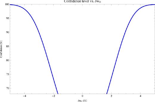
The confidence level of a possible detection of SR DE versus δw0 ≡ w0 − 1, neglecting errors in the cosmological parameters. It is very encouraging to note that even if the deviation from a cosmological constant is only at the 2 per cent level, we might expect, in the limit of highly accurate cosmological parameters (specifically, as Section 5 will discuss, the matter density and Hubble constant), a detection at approximately 75 per cent confidence. If δw0 = 3.5 per cent, the confidence of a detection would rise to 96 per cent.
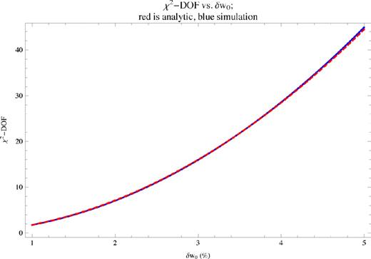
The red dashed curve shows the analytical formula (equation 24) and the blue solid curve the numerical results. The vertical axis shows the χ2 minus the number of degrees of freedom (DOF). This shows that our analytical scaling for χ2 is an extremely accurate predictor of the true numerical values. This plot assumes no error in the cosmological parameters.
In case (ii), we simply add a 1 per cent uncertainty in H0 from all non-DE experiments to our work. We expect this to be an overestimate. This is the simplest approach. Considering possible correlations between the errors in H0 and Ωm, which for instance would occur if the measurement of Ωm came from Ωmh2and the uncertainty in h were not negligible compared to that in Ωm, is beyond the scope of this work, as the precisions that future experiments will be able to achieve on these parameters may only be estimated at present in any case. We do display the confidence level of a detection for different values of δw0 as a function of the precision on Ωm, with 1 per cent precision on H0 from all non-DE experiments, in Appendix A3. This is to illustrate that, for reasonable expected values of the precision on Ωm, even if they differ from 1.25 per cent, one can still expect a detection with good levels of confidence.
We now turn to discussion of case (i) in the following section and case (ii) in Section 5.3.2.
In current densities
Our model is motivated by inflation, which implies a flat Universe. If inflation is persuasive, then the reader will believe that the Universe really is flat, meaning spatial curvature is actually zero to high accuracy. This also means we are at the critical density today, so the densities of matter, radiation and DE must sum to unity. The radiation density is 10−5 today, so we neglect it; this approximation will never be a significant source of error at the redshifts we consider, as we have noted earlier several times. We therefore have the constraint that ΩDE + Ωm = 1, which means that an overestimate of DE will correspond to an underestimate of matter, and vice versa. Because this is so, we need not directly consider errors in the DE density. Should one desire the effects of an overestimate of x per cent in the DE density, one just needs to consider a corresponding underestimate of the matter density, given by −2.7x per cent, because ΩDE → (1 + x)ΩDE, so Ωm → (1 − xΩDE/Ωm)Ωm = (1 − y)Ωm, with y = x(ΩDE/Ωm) ≈ 2.7x.
We use a projected precision on Ωm today of 1.25 per cent from Planck; see Section 3.1. This is the uncertainty in Ωmh2 which Planck will obtain. If an accurate value of h ≡ H0/(100 km s−1 Mpc−1) is obtained by other experiments, then we should know Ωm at least this accurately.
For instance, we can determine h to an accuracy of 1 per cent from the Planck CMB data alone, with the flatness assumption. BOSS and BigBOSS alone, together with model fitting of the dark matter model, should lead to a value of h with a statistical uncertainty of 0.3 per cent. Given the 0.193 per cent uncertainty in rs, this would give an uncertainty in h of 0.48 per cent from BOSS and BigBOSS alone. Therefore, combining measurements of h from the Planck CMB data and from BOSS and BigBOSS should yield an estimate of h with an accuracy of 0.43 per cent.
Other improvements in h could come from SN measurements, gravitational lensing time delays and gravity wave detections from Laser Interferometer Space Antenna (LISA) (if its original funding were restored) (Phinney 2002). Hence, we will assume improvements in h measurement over the next seven years, using these methods and others, to be sufficient that uncertainty in h is not the limiting factor in determining Ωm.
Further, we note that Ωm may be measured independently using masses of CL of galaxies calibrated by large N-body simulations. Ωm can also be measured using the amplitude of large-scale velocity perturbations. These points bolster our claim that it is conservative to estimate that Ωm may be measured to 1.25 per cent. For additional discussion of the effects of errors in Ωm, see Alam, Sahni & Starobinsky (2007) and Sahni, Shafieloo & Starobinsky (2008).
In the Hubble constant
We now turn to the Hubble constant. All BAO and topology measures of dA(z)/dA(z = 1089) are to be compared with models. This is because dA(z = 1089) can be determined to high accuracy (0.2 per cent) from the CMB. Likewise, SN measurements of dA (from dL) can be compared with each other. Distant SNe can be compared with nearby ones to determine relative values of dA(z) normalized by nearby SNe. Thus, in both cases, uncertainty over the value of H0 = 73.8 ± 2.4 km s− 1 Mpc− 1 (Riess et al. 2011), which is currently at the 3.3 per cent level, can be eliminated.
However, direct measurements of the Hubble constant, such as those to be done by WFIRST, Euclid, BOSS and BigBOSS, are sensitive to uncertainty in the value of H0. These data points constitute 65 per cent by number of the points we use in our analysis, so we must incorporate the possible effects of an error in H0. We take it that in the next five years, H0 will be constrained to a precision of the order of 1 per cent (Page, personal communication), and use this value to compute the χ2 penalty a value of H0 different from the current best value will incur in our simulations.
Method
Our concern is to understand the effects of an error in H0 or in Ωm on the observations. If the true cosmology were SR DE, but an error in H0 or in Ωm (or both) were made and a cosmological constant cosmology assumed, might the error mimic the effect of SR DE and thus allow the (false) cosmological constant cosmology to fit the observations well?
We calculate the difference between observables, such as the angular diameter distance and Hubble constant, for a w ≡ −1 cosmology with incorrect values of H0 and Ωm and an SR DE cosmology with the correct H0 and Ωm, which we take to be Ωm = 0.272 from the WMAP-7+BAO+H0 value and H0 = 73.8 ± 2.4 km s−1 Mpc−1 from Riess et al. (2011). The precisions and experiments used are described in detail in Section 5.2, and summarized in tables in Appendix B.
For a given δw0 and H0, we sample a number of ‘wrong’ values of Ωm. The results for several δw0's are displayed as solid curves in Fig. 6. The minima of the parabolas in that figure are the Ωm's in a cosmological constant cosmology that will best ‘mimic’ SR DE cosmologies with values of δw0 as given on the horizontal axis and a correct value of H0. They will hence be the values that, given the correct H0, make it most difficult to distinguish the two different cosmologies.
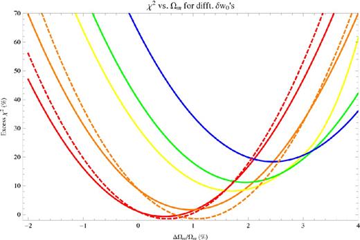
Red is δw0 = 1 per cent, orange 2 per cent, yellow 3.5 per cent, green 4 per cent and blue 5 per cent. Solid curves denote numerical results and dashed curves those using analytical formula (equation 27). We have only plotted the analytical scaling for two curves so that the plot remains legible.
We now momentarily restrict ourselves to errors in Ωm only, and assume that we have the correct value for H0. We discuss several numerical checks done on these results below, considering as a typical example the SR case with δw0 = 3.5 per cent. Following this discussion, in Section 5.3.7 we return to the main thread of Section 5.3 and detail how uncertainty in H0 is incorporated.
For δw0 = 3.5 per cent, the ‘mimic’ matter density, denoted with an additional subscript ‘m’, is Ωmm = 0.278 392, 2.55 per cent larger than the true value of Ωm. If the true cosmology were w ≡ −1 but with this value of Ωm, there is a 27 per cent chance that we would mistakenly see observational results that mirrored an SR DE cosmology with Ωm = 0.272 and δw0 = 3.5 per cent.
Why is the mimic value of Ωm larger than 0.272? SR DE has a higher average value of w than does cosmological constant DE. Having w ≡ −1 but with an overestimate of matter relative to the true value has the effect of raising wtot, the average total ratio of pressure to energy density, because matter has w = 0. SR DE has w > −1, so it also has this effect. Thus, it is no surprise that extra matter can mimic SR DE. Too much extra matter, though, leads to a χ2 penalty into the past, as the SR DE cosmology diverges from the w ≡ −1 (with wrong Ωm) cosmology in the matter-dominated epoch when that wrong amount of matter becomes more dominant.
We now discuss three methods we use to check the plausibility of our numerical results.
Small-z expansion
Average total equation of state today
Secondly, one may define |$\bar{w}_{\rm {tot}}=\sum \Omega _i w_i/\sum \Omega _i$| and ask for what Ωmm is so that |$\bar{w}_{\rm {tot},\,{\rm SR}}=\bar{w}_{\rm {tot},\,w\equiv -1}$|, where a subscript ‘tot’ denotes the total ratio of pressure to energy density. In other words, at present, what Ωmm is required in the w ≡ −1 cosmology so that the overall ratio of pressure to energy density is the same as that in the SR DE cosmology? This leads to the same result as given in equation (26). This is unsurprising as equation (26) is from a small-z expansion about z = 0, the present.
Evaluating equation (26) yields Ωmm = 0.297 48. From earlier in this section, the numerical Ωmm = 0.278 392. Recall that the latter value is obtained by finding the χ2 for all the proposed future observations as a function of Ωm and seeing which value of Ωm in a cosmological constant cosmology best mimics an SR model with δw0 = 3.5 per cent. So we would expect these results to be very close to each other. However, the analytical result from equation (26) is farther above the true value of Ωm = 0.272 because the analytical analysis includes only small redshifts z ≪ 1, whereas the numerical results include the past out to z ≃ 2. Being wrong on Ωm increases the χ2 more and more as one goes further back into the past, so we would expect that the numerical Ωmm is closer to the true value of Ωm than the analytical Ωmm from equation (26) is. To check that intuition, we compute a numerical Ωmm by the methods described above but using only observations z ≤ 1. We would expect this result to be higher than Ωmm as computed using the full set of observations (i.e. including higher redshift observations) because it will not be paying the χ2 penalty of being more and more wrong farther back in the past, since points with z > 1 are not included. We also expect it to be closer to Ωmm as from equation (26) because that equation is valid for small z and Ωmm will now be computed using only small z (z < 1). The value obtained is Ωmm = 0.278 853, which fulfils these expectations.
Finally, we can even fit a line to the two points from the numerical analysis (all z, and z < 1 only) as a function of |$\bar{z}$|, the average redshift of the observations used. In other words, it is the line that fits both |$(\bar{z}_{{\rm full}},\Omega _{{\rm mm}})$| and |$(\bar{z}_{{\rm small}},\Omega _{{\rm mm}})$|, where the former Ωmm is from the full numerical χ2 with all observations as described earlier in this section and the latter is from the small-z only subset as described in the previous paragraph. The line fitting these two points can then be used to extrapolate and find a prediction for the value of Ωmm if only today (z = 0) were taken into account. This result is Ωmm, 0 = 0.279 397, larger than both Ωmm for small z and the numerical result for Ωmm, as expected, and closest of this set to the value from equation (26).
Comparison with analytical χ2 scaling
Now, observations of H represent 65 per cent of the observations we use, so we expect the scaling to be good but not perfect. It is both this point and the fact that we evaluate A(u) at an average value of u = 1 + z = 2 that cause the analytical formulae to be shifted slightly to the right of the numerical results in Fig. 6. Indeed, one can calculate χ2 using only Hubble constant measurements to eliminate the former point; even then the analytical results do not perfectly mirror the numerical ones, showing that evaluating A(u) at an average redshift does introduce some error. However, the analytical results agree well enough with the numerical results to persuade that the latter are accurate.
Adding uncertainty in H0
We iterate the process described in Section 5.3.3 over different values of the Hubble constant H0. Ultimately, we thereby obtain a hyper-surface giving χ2 as a function of δw0, the error in the matter density ΔΩm, and the error in the Hubble constant ΔH0. We show several representative slices through this hyper-surface in Section 6, Figs 8–10.
To obtain the confidence with which SR DE might be detected for a given δw0, we calculate the value of ΔH0 and ΔΩm for which χ2 is minimized. In other words, we ask, for each value of H0 and δw0, what Ωm minimizes the confidence of a detection. Then, we allow the value of H0 to vary to minimize over this set. This gives the minimum confidence of a detection for a particular δw0. Essentially, at a given δw0, we look at many slices of constant H0, for instance as given in Figs 8–10, and find the Ωm lying on the lowest confidence ellipse in each slice. We then seek the slice of constant H0 for which the confidence associated with this point will be least. This procedure yields the least favourable combination of Ωm and H0 for distinguishing SR DE with a given δw0 from a cosmological constant DE cosmology with different cosmological parameters. The resulting confidences are plotted in Fig. 11.
The checks described in Sections 5.3.4 and 5.3.5 do not apply to uncertainty in H0, since term-by-term equality in powers of z in equation (28) is no longer possible if H0 differs between the SR and cosmological constant cosmologies. However, the same type of check as that described in Section 5.3.6 does apply; we derive a scaling formula (equation A53) in Appendix A4, and compare it with the numerical results in Fig. 7. The agreement should persuade that the numerical results are accurate.
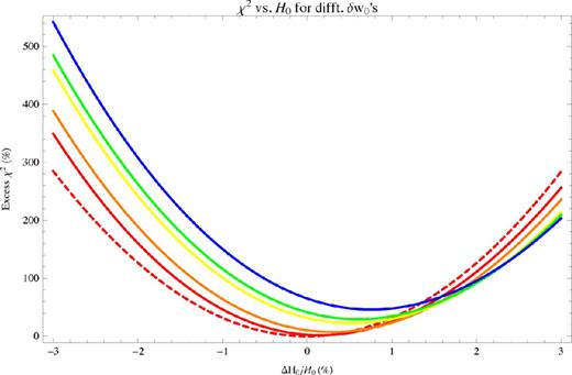
Red is δw0 = 1 per cent, orange 2 per cent, yellow 3.5 per cent, green 4 per cent and blue 5 per cent. Solid curves denote numerical results and dashed curve that using analytical formula (equation A53). We have only plotted the analytical scaling for one curve so that the plot remains legible.
RESULTS
Using the method outlined in the previous section, we calculate the least favourable combination of errors ΔΩm and ΔH0 for distinguishing an SR DE cosmology from a cosmological constant cosmology for each δw0 we study. These are the errors ΔΩm and ΔH0 in a cosmological constant cosmology that would best mimic an SR DE cosmology with Ωm = 0.272 and with a certain value of δw0. Hence, this is the cosmological constant cosmology that would be hardest to distinguish from an SR DE cosmology with Ωm = 0.272. Thus, it will produce the lowest χ2 and the lowest confidence level of detection.
We hope that the confidence levels our analysis yields will show the value of funding as many experiments as possible. Given that this may not occur, however, we also provide several breakdowns of the χ2 contributions, which may be helpful in assessing which experiments will yield the greatest evidence for or against SR DE. We provide the individual χ2 for each experiment (Table 2), bin them into space based and ground based (Table 3), and bin them into experiments beginning in the next five years and experiments beginning six years from now or later (Table 4). In the first of these tables, we show the values obtained neglecting errors in the cosmological parameters as well as those obtained accounting for them.
χ2 for individual experiments if δw0 = 3.5 per cent. The confidence level is one minus the probability of getting w ≡ −1-like observations by chance if SR DE is the true cosmology. The third column assumes that we know the cosmological parameters Ωm and H0 to arbitrary accuracy. The final column, ‘χ2 w/errs.’, shows the χ2 value of a detection (and the bottom row the confidence of a detection) when the possibility of errors in the matter density Ωm and the Hubble constant H0 has been accounted for as described in Section 5. The value in the ‘χ2 w/errs.’ column for ‘Wrong H0’ is actually 1.0034, so we have accounted for the possibility of a wrong H0 (and wrong Ωm); in contrast, in the ‘χ2’ column, these parameters are both constrained to have the correct values.
| Experiment | DOF | χ2 | χ2 w/errs. |
|---|---|---|---|
| BOSS dA | 3 | 3.56 | 3.20 |
| BOSS H | 3 | 3.38 | 3.29 |
| LSST BAO/WL | 9 | 19.88 | 10.67 |
| WFIRST SNe | 11 | 14.27 | 12.23 |
| WFIRST H | 13 | 14.83 | 13.50 |
| EuclidH | 12 | 13.26 | 12.17 |
| BigBOSS H | 16 | 19.63 | 16.60 |
| Wrong matter | 1 | 1.00 | 2.99 |
| Wrong H0 | 1 | 1.00 | 1.00 |
| Total | 69 | 90.81 | 75.65 |
| Confidence | – | 95.96 per cent | 72.75 per cent |
Contribution to χ2 of ground-based or space-based observations each, with δw0 = 3.5 per cent. We have split the matter and H0 contributions equally between ground- and space-based experiments, as each parameter will be constrained by both and a more sophisticated split would be unnecessarily complex.
| Experiment | Per cent of χ2 w/errs. |
|---|---|
| Ground | 47.53 per cent |
| Space | 52.74 per cent |
| Experiment | Per cent of χ2 w/errs. |
|---|---|
| Ground | 47.53 per cent |
| Space | 52.74 per cent |
Contribution to χ2 of experiments in the next five years only or in six years plus, with δw0 = 3.5 per cent. We have counted the matter and H0 contributions as coming solely from observations in the next five years, as the precisions we have used for these are expected to be achieved in that timeframe.
| Experiments in | Per cent of χ2 w/errs. |
|---|---|
| Next five only | 51.88 per cent |
| Six plus only | 48.12 per cent |
| Experiments in | Per cent of χ2 w/errs. |
|---|---|
| Next five only | 51.88 per cent |
| Six plus only | 48.12 per cent |
Figs 8 –10 show the confidence level resulting from the χ2 analysis versus δw0. Fig. 11 condenses these results into a single curve giving the confidence values as a function of δw0 for the least favourable values of ΔΩm and ΔH0. What is encouraging is that, even assuming the worst-case scenario that our values of the matter density and H0 are incorrect in precisely the way least favourable to distinguishing SR from cosmological constant DE, for the value δw0 = 3.5 per cent, we may still expect a detection at 70 per cent confidence using experiments taking place in the next seven or so years. Furthermore, should δw0 be larger (e.g. 5 per cent), a possibility still very much observationally allowed, the confidence of a detection might rise to ≃85 per cent.
Figs 8–10 show the confidence values as a function of the per cent change in matter density and the per cent change in δw0, the latter being equal to δw0 because δw0 is already normalized to w = −1. There are two key points here. First, one can view the ratio of the axes of the ellipse as an effective measure of how strongly each parameter (Ωm and δw0) comes into the final confidence estimate. We focus now quantitatively on Fig. 8, though our comments will apply qualitatively to Figs 9 and 10 as well. The ratio of semimajor to semiminor axes is ≃2.9, meaning roughly that a given fractional change in Ωm will have about three times the effect on the confidence value that the same fractional change in δw0 would have. This is unfortunate because it essentially means the observations are more sensitive to the value of Ωm than to the DE equation of state! More concretely, this can be conceived as follows. Suppose one is certain about Ωm and believes one has detected δw0 = 2 per cent with confidence such that one is in the red region of the plot. Now suppose one realizes there in fact is some uncertainty about Ωm. Since the ellipse is tipped, it does not take much movement in Ωm to move from the red region of the plot, where one has a high-confidence detection, to the blue region of the plot, where one has much less confidence.
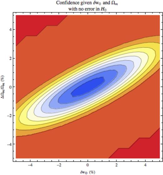
The confidence of a detection as a function of δw0 and Ωm assuming no error in H0. Warmer colours denote a higher confidence detection of SR DE; the scale should be read just like a thermometer. The orange ellipse intersecting (−5, −3.5) is 95 per cent confidence, the white ellipse 75 per cent and the centre blue 55 per cent.

The confidence of a detection as a function of δw0 and Ωm assuming a 3 per cent error in H0. Warmer colours denote a higher confidence detection of SR DE; the scale should be read just like a thermometer. The orange ellipse intersecting (−5, −3.5) is 95 per cent confidence, the white ellipse 75 per cent and the centre blue 55 per cent.
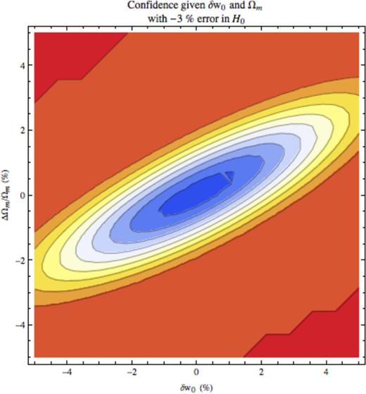
The confidence of a detection as a function of δw0 and Ωm assuming a −3 per cent error in H0. Warmer colours denote a higher confidence detection of SR DE; the scale should be read just like a thermometer. The orange ellipse intersecting (−5, −3.5) is 95 per cent confidence, the white ellipse 75 per cent and the centre blue 55 per cent. Note that this plot is very similar to that for an overestimate for H0 of 3 per cent; this illustrates that the χ2 depends mainly on the magnitude of the error and not the sign. However, the scaling (equation A53) of Appendix A4 shows that there is also a small contribution to the χ2 from a term linear in ΔH0/H0; this term will allow the sign of the error in H0 to affect the results. It is this that underlies the slight differences between this figure and Fig. 9, which may especially be seen around ΔΩm/Ωm ≃ 4 per cent and δw0 ≃ −4 per cent.
Secondly, the ellipse's major axis is offset by an angle of ≃ π/7 rad from the δw0 axis. This is a result of coupling between Ωm and δw0, a coupling introduced because we have constrained Ωm + ΩDE = 1, so ΩDE = Ωm − 1. This coupling contributes to the fact that there exist particular erroneous values of Ωm that can mimic the effect of a given δw0. The physical reason for the latter point, as we have already noted, is that matter has equation of state p/ρ = 0, so adding extra matter pulls the average equation of state in a cosmological constant model up towards zero from −1. SR DE with δw0 > 0 has equation of state p/ρ > −1, so it may be mirrored by adding extra matter in a cosmological constant cosmology. Phantom DE with δw0 < 0, which has an equation of state p/ρ < −1, may analogously be mirrored by an underestimate of the matter density, letting the average total equation of state in a cosmological constant model tend closer to −1.
Equation (29) encodes two effects. First, as we have already discussed, the confidence is more sensitive to the matter density than to the DE equation of state, so one needs to move less in matter to mirror a given move in equation of state; this is the factor of (a/c). Secondly, because the matter and DE densities are coupled by the flatness constraint, the DE equation of state will be coupled to the matter density (also as noted above). Thus, moving along the matter density–error axis is not the most efficient way of moving from one confidence contour to another on the ellipse: i.e. changing only the error in the matter density does not change the confidence of a detection as much as it would were there no coupling. The most efficient route would be along the semiminor axis of the ellipse, which is a gradient of the contour plot as is evident because it is perpendicular to the contours. Because the axes of the plot do not align with this most efficient route, one pays a penalty of cos (θ): for a given change in matter density ΔΩm, the δw0 this mimics will be suppressed by a factor of cos (θ).
Fig. 11 takes the minimum confidence value associated with each δw0 as the confidence with which a detection of that value might be claimed (see Section 5.3.7 for details of this minimization). Fig. 11 shows that if δw0 = 3.5 per cent, a detection at 73 per cent confidence should be possible with upcoming experiments even if we are wrong about the matter density and H0 in the least favourable way for detecting SR DE. If δw0 = 5 per cent, a possibility still very much observationally allowed, then the confidence of a detection even in this worst-case scenario would rise to ≃85 per cent.
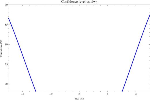
The confidence level to which a detection of SR DE is possible accounting for the possibility of errors in Ωm and H0.
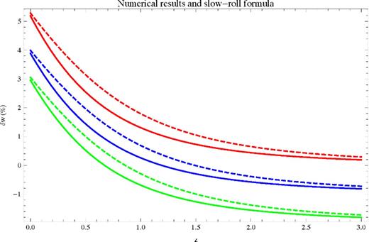
Scalar field: the solid curves denote the results of an exact, self-consistent numerical solution of the Friedmann equation and scalar field EOM for several typical potentials. Dashed denotes the SR formula (equation 9) evaluated using equation (14) for the Hubble constant (i.e. equation 15). Red is for a quadratic potential, blue for a quartic potential and green for an exponential potential. All curves correspond to δw0 ≈ 5 per cent; we have shifted the quartic result down by a constant 1 per cent and the exponential result down by a constant 2 per cent so that all three curves are clearly visible. The quadratic test was done in Gott & Slepian (2011).
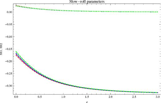
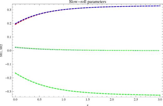
Scalar field: these show the two SR parameters for each potential. Red is quadratic, blue is quartic and green is exponential. Dotted is SR1 (all greater than zero) and dashed is SR2. All three curves overlap for SR1 so that they are indistinguishable; they also overlap for SR2 but can be distinguished. The key point is that all of the curves have a magnitude much less than unity, meaning the fields are in SR.
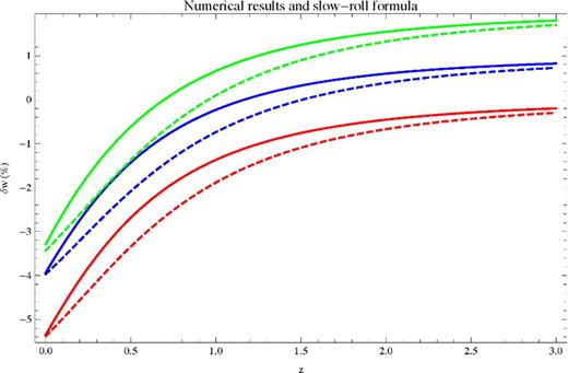
Phantom: the solid curves denote the results of an exact, self-consistent numerical solution of the Friedmann equation and phantom field EOM for several typical potentials. Dashed shows the SR formula (equation 9) evaluated using equation (14) for the Hubble constant (i.e. equation 15). Red is for a quadratic potential, blue for a quartic potential and green for an exponential potential. All curves correspond to δw0 ≈ 5 per cent; we have shifted the quartic result up by a constant 1 per cent and the exponential result up by a constant 2 per cent so that all three curves are clearly visible.
Phantom: these show the two SR parameters for each potential. Red is quadratic, blue is quartic and green is exponential. Dotted is SR1 (these curves begin with values ≃ 0.02 for z = 0) and dashed is SR2. All three curves overlap for SR1 so that they are indistinguishable; two of the three also overlap for SR2 but can be distinguished. The key point is that all of the curves have a magnitude much less than unity, meaning the fields are in SR.
CONCLUSION
In this paper, we have made two major arguments. First, we have suggested that, if DE is not a cosmological constant with equation of state w ≡ −1, the simplest alternative would be that it is a second epoch of inflation, driven by a mechanism similar to that likely behind the first – a scalar field slowly rolling down the hill of its potential (i.e. in SR). Should Planck detect the tensor mode amplitude predicted by e.g. Linde's chaotic inflation, that would be smoking-gun evidence for a first epoch of inflation. If that occurs, the prospect that DE may be a second epoch of inflation driven by an analogous mechanism should be taken seriously.
We have here developed this idea to show that in such a DE model, the Hubble constant will have a generic evolution with redshift that is relatively insensitive to the starting value of the field's potential or the shape of the potential, and dependent solely on the difference from −1 in the DE equation of state today. This differs from previous work in that previous work (e.g. Crittenden et al. 2007; Chiba 2009; Novosyadlyj et al. 2010) derived two-parameter forms for w. By showing that w is insensitive to the scalar field's acceleration as long as the acceleration is either small or roughly constant, in this work we have obtained a one-parameter model for w.
We have used this result to assess whether observations upcoming in the next decade will be able to distinguish between SR DE and cosmological constant, w ≡ −1, DE. The current error bars from WMAP-7+BAO+H0 constrain w0 to be near −1 at roughly the 10 per cent level; we have been even more conservative in our estimates and considered deviations from w = −1 at present of ≲5 per cent. We find that, neglecting errors in the cosmological parameters H0 and Ωm, if DE is a field in SR with w + 1 = 3.5 per cent today, this would be detectable to 96 per cent confidence by observations in the next decade. Accounting for the current error bars on the cosmological parameters H0 and Ωm, this picture worsens somewhat. For reasons we present in Section 5, we find that, assuming a flat cosmology (motivated by inflation), the confidence level of a detection of w different from −1 is only affected by errors in the matter density and H0 today. Detailed numerical modelling of the effects of such errors shows that a difference from w = −1 of 3.5 per cent could be detected with 73 per cent confidence (see Fig. 11). We have quantified the error introduced in our form for H(z) (equation 14) due to the approximation new to this work, and shown that (Fig. A8) for a ϕ2 potential the error will be an order of magnitude less than the signal. Since our analytical form (equation 51) for this error bound is generic to other potentials, and to order of magnitude matches the numerical results for V ∝ ϕ2 (see Fig. A7), the error introduced by our approximation should also be negligible compared to the signal for other potentials.
There is a second, parallel main thread to this work as well. As noted in the introduction, there are numerous time-varying physical models of DE. Because testing each model individually would be overwhelming, parametrizations have been proposed that give the redshift evolution of w once their parameters have been fixed. Each physical model may then produce predictions for the parameters in these parametrizations. However, such parametrizations often build in a shape for the redshift evolution of w that has little physical motivation. Therefore, a formula that is physically motivated but still able to test a broad class of models is desirable. We suggest that equation (14) of this work satisfies these desiderata. As we have shown, it will apply to quintessence models of DE (these are the most analogous to the mechanism of inflation), and also to phantom DE, as long as in each model the field is, as expected, in SR. We already know from observation that one of the two conditions required for SR is satisfied today: since in all of these models, w + 1 is proportional to the square of the field's velocity, the tight constraints on w's deviation from −1 demand the field's velocity today be small.
We have shown that, for both quintessence and phantom DE in SR, equation (14) will describe the evolution of the Hubble constant with redshift. Thus, our calculations of the confidence with which SR DE may be distinguished from a cosmological constant have broad implications: if DE is in SR, we may expect an observational detection with some confidence in the next decade, dependent on the value of w + 1 today.
With this formula in hand, observers may be able to extract a signal from otherwise too noisy data: this is because the shape of w(z) in our formula is physically motivated; therefore, whether the observations fit this shape provides additional information over and above the absolute amplitude of the curve, which is just set by δw0 = w + 1 today. Because our formula has only one free parameter, δw0, it is more easily tested against observations than the two-parameter models typically favoured (e.g. the Chevallier-Polarski-Linder parametrization) because it will be quickly evident if the prediction for w(z) in the past implied by δw0 today is not fulfilled. Furthermore, with the shape for w(z) our formula gives, data on w(z) in the past may be used to tighten the constraints on w today. This is because these data, if fitted with the shape our formula implies, will demand a unique value of w today.
This work also points out that improvements in independent measurements of H0 and Ωm are very important to the study of DE. Original methods such as the original LISA proposal for measuring H0 (before its budget was cut) and measures of Ωm from peculiar velocities and gravitational lensing, to name just a few, should be encouraged. They provide important support work for the exciting DE observational programmes now proposed.
ZS thanks Paul Steinhardt, Daniel Eisenstein, Neta Bahcall, Harvey Tananbaum, Stephen Portillo, Philip Mocz, Aisha Down and Laura Kulowski for many helpful conversations during the course of this work. ZS particularly appreciates the willingness of the first on this list to be both critic and sounding board. All authors thank Michael Blanton for helpful comments during revision. This material is based upon work supported by the National Science Foundation Graduate Research Fellowship under Grant No. DGE-1144152.
Equation numbers have been corrected in the Appendix.
For instance, we would argue that DE is unlikely to be driven by a phantom field. Inflation certainly was not driven by a phantom field, for had it been we would not be here, as a ‘big rip’ would have already occurred (Caldwell 2002; Caldwell, Kamionkowski & Weinberg 2003). Importantly, this comment also applies to the current ‘standard’ model of DE, as a constant vacuum energy density (cosmological constant) with w ≡ −1. In this model, the current Universe sits stationary at the bottom of a potential well with a value of V0 = 10−120 in Planck units (Weinberg 1987; Vilenkin 2003). However, if DE is just another epoch of inflation, neither inflation nor DE can be due to a constant energy density, or we would not be here – the Universe would still be undergoing high-speed inflation!
For a review of previous DE models, with a focus on those most similar to that proposed here, see Gott & Slepian (2011). A brief review of the evidence for inflation may also be found there.
Our results will hold for any field where DE is provided by the scalar field's potential and the SR conditions are met; importantly, our results will not apply to k-essence models, where DE is provided by the scalar field's kinetic energy (cf. Armendariz-Picon, Mukhanov & Steinhardt 2001). For discussion of SR thawing k-essence models, see Chiba, Dutta & Scherrer (2009).
Chiba, Siino & Yamaguchi (2010) obtain a similar parametrization for a non-minimally coupled scalar field.
As we discuss in Sections 1.1 and 7, there has been much previous work to derive the analogues of the inflationary SR conditions for scalar field DE, particularly the work of Chiba (2009) giving the SR DE analogues of the inflationary parameters ϵ ≡ 1/2(V′/V)2 ≪ 1 and η ≡ V′′/V ≪ 1 (equivalent to |${\rm SR}1\equiv \dot{\phi }^2/2V\ll 1$| and |$|{\rm SR}2|\equiv |\ddot{\phi }/(\mathrm{\partial} V/\mathrm{\partial} \phi ) | \ll 1$|). He shows that |$|\beta | \equiv | \ddot{\phi }/3H\dot{\phi } |$| is either negligible compared to unity (for freezing models; see Caldwell & Linder 2005) or roughly constant (for thawing models). The EOM gives |$\dot{\phi }=-V^{\prime }/3(1+\beta )H$|, so for either case as long as V′ is roughly constant we recover |$\dot{\phi }\propto 1/H$|, as we would expect since SR2 contains information about |$\ddot{\phi }$|, as does β. In contrast to this work, Chiba does not argue that V′ is roughly constant, nor that this, in conjunction with the behaviour of β, means |$\dot{\phi }\propto 1/H$|.
Note that if δw ∝ H−2, as we have shown, the approximation δw ≪ 1 becomes even better in the past because H rises in the past.
See Eisenstein (2013) for more pedagogical discussion of this calculation.
REFERENCES
APPENDIX A:
Self-consistency of the approximations of Section 2, and numerical results
In a single-component universe with only DE, the approximation that H evolves more in time than ∂V/∂ϕ would not be correct, as |$H\propto \sqrt{\rho }\approx \sqrt{V}$|. For instance, for a quadratic potential, H ∝ ϕ and ∂V/∂ϕ∝ϕ as well. Similarly, in inflationary cosmology, this approximation would be incorrect because the inflation field is the sole non-negligible source of the energy density. However, for z ∼ 0-2, matter also determines the time evolution of H. Thus, H may evolve in time even if V and ∂V/∂ϕ do not, and the approximation is self-consistent.
The first equality uses the chain rule, while the second uses the relation directly after equation (4) to replace ∂V/∂ϕ with |$-3H\dot{\phi }/(1+{\rm SR}2)$| and then that |$\delta w\approx \dot{\phi }^2/V$|. The final bound uses a ≤ 1, δw ≤ δw0 ≤ 0.05 and min SR2 = −1/3, the last from Figs A2 and A4. Note that in the limit that SR2 ≪ 1, which holds as z → 0, the bound becomes sharper: 0.225 becomes 0.15.
Comparing equations (A2) and (A3) shows that for a field in SR, our approximations in Section 2 will hold. This analysis also applies to phantom DE. In those models, the EOM for the field, and δw, differs only in sign from standard scalar field models. Our analysis here is sensitive to the magnitudes of quantities but not their signs.
We now present several figures (Figs A1 –A4) illustrating how well the approximate formulae equations (14) and (15) work for typical potentials in each model. Here our goal is not to provide comprehensive coverage of every possible initial condition or potential, but rather to offer examples to supplement and bolster the analytical work we have already discussed. We briefly detail the numerical method used to obtain these figures later in this appendix (Appendix A6).
We plot the SR parameters (defined following Lesgourgues 2006) |${\rm SR1} \equiv \frac{1}{2}\dot{\phi } ^2/V$| and |${\rm SR2} \equiv \ddot{\phi } /(\mathrm{\partial} V /\mathrm{\partial} \phi )$| in Figs A2 and A4; these show that the fields actually are in SR for typical potentials in each model we simulate. Figs A1 and A3 show the applicability of equation (15) to typical models.
Validity of the approximations of Section 2
when SR2 varies noticeably with redshift, which occurs for z < 1, and
when SR2 is nearly constant and approximately equal to −1/3, which occurs for z ≳ 1.
In each regime, to verify our scaling |$\dot{\phi }\propto 1/H,$| we must check two conditions:
that SR2's explicit presence above does not invalidate the scaling, and
that SR2 does not cause ∂V/∂ϕ to vary comparably to 1/H.
We have already checked (ii) for both regime (1) and regime (2) in Appendix A1, so we here focus on (i).
We plot this using s = −0.15 and s0 = −0.15 in Fig. A5.
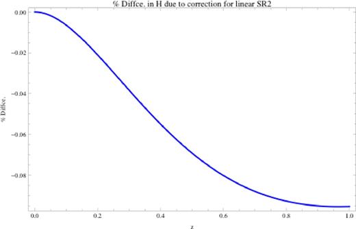
δH (per cent) as given by equation (51).
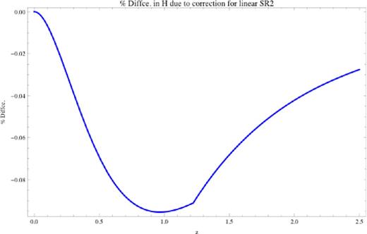
δH (per cent) as given by equation (51), extended to regime (2) as explained in the text.
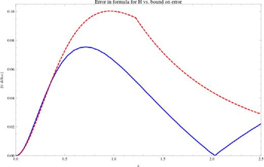
Here we plot the absolute values of the error between our formula for H (equation 14) and the exact numerical results for δw0 ≃ 4 per cent (blue solid) and the bound on this error given by equation (51) and extended as explained in the text (red dashed). The cusp in the numerical results is because the error goes negative for z > 2 and we have taken an absolute value. Note that the precise behaviour of the error of our formula here should be unimportant because these points contribute little to the χ2, both because few observations go to z > 2 and because DE becomes subdominant to matter for z ≳ 2.
We now treat regime (2), where SR2 ≈ const ≈ -1/3. Note that we have chosen a specific normalization for the scaling δw ∝ 1/H2 by setting it to δw0 at z = 0. This incorporates the constant s0 in our expansion for SR2 in regime (1), but here SR2 ≈ const = −1/3 ≠ s0. The fact that SR2 now becomes a constant not equal to s0 means that |$\delta w=\delta w_{0}H_{0}^{2}\chi /H^{2}(z)$|, where χ accounts for the fact that the scaling now must have a different constant of proportionality. We may easily obtain the error by letting z = 1.22 in the numerator of |$\Delta H_{{\rm SR2,lin}}^{2}$| in our relation for δH, because at this z SR2 = 1/3, and SR2 is a continuous function at the boundary between the two regimes. H2(z) in the denominator of |$\Delta H_{{\rm SR2,lin}}^{2}$| continues to increase with z, however. Thus, we may extend our error plot out to higher z. See Figs A6 and A7. In Fig. A8, we compare the error in H due to our formula being approximate to the signal we seek (the difference between SR and cosmological constant cosmologies), showing that this signal is always approximately an order of magnitude larger.
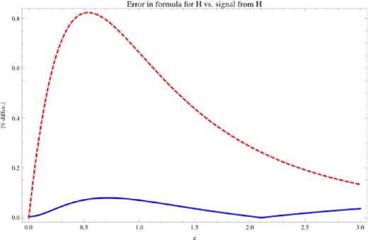
Here we plot the absolute value of the error in H between our formula (equation 14) and the exact numerical results (blue solid) as compared to the difference between our SR formula for H and a cosmological constant H, the signal we hope to detect (red dashed). For z ≲ 2, the error is always approximately an order of magnitude less than the signal, meaning our formula (equation 14) will be a fairly accurate descriptor of how an SR DE model differs from a cosmological constant DE model.
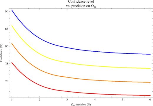
These curves show how the confidence of a possible detection (assuming 1 per cent precision on H0) changes as a function of the precision on Ωm. From top to bottom, the curves correspond to δw0 = 5, 4.5, 4 and 3.5 per cent.
Fractional differences in Hubble constant and comoving distance
Scalings for χ2
The second term on the right-hand side of equation (A41) comes from evaluating I[u], which is the indefinite integral resulting from equation (44), at the lower bound z = 0. 2F1 and 3F2 are generalized hypergeometric functions.
Finally, we provide Fig. A5 to show the effects of changes in the precision to which Ωm is measured on the confidence of a detection of SR DE.
Reconstruction of confidence ellipse
Numerical method for Appendix A2
We now have two coupled equations to solve (equations A56 and A57); this is done using Mathematica's built-in NDSolve routine. We set the initial conditions at a very small value of time and scalefactor obtained from explicit numerical integration of the Friedmann equation with a cosmological constant DE; this is to avoid the singularity in H(τ) at τ = 0 otherwise encountered in equation (A57). So doing will introduce negligible error because DE is exceedingly subdominant to matter and radiation at the value we choose, a = 10−10.
We specify initial conditions at a = 10−10 using the insight that, since the field should be in SR, it will not change much from then until now. Thus, to obtain the correct DE density and desired δw ≃ 5 per cent now, we may set the corresponding values of V0 and |$\phi ^{\prime }_0$| (at present) as initial conditions at a = 10−10. This first guess for the initial conditions does not yield precisely the correct DE density or δw today, so we then change the initial conditions slightly and iterate until we achieve δw ≃ 5 per cent and ΩDE = ΩDE0. This process converges quickly and yields self-consistent, exact solutions to the coupled system. These results are plotted in Figs A1–A4. See also Gott & Slepian (2011).
APPENDIX B: TABLES OF PRECISIONS USED
WFIRST SN luminosity distance (optimistic) (Green et al. 2012).
| z | Precision |
|---|---|
| 0.17 | 0.018 |
| 0.25 | 0.011 |
| 0.35 | 0.009 |
| 0.45 | 0.008 |
| 0.55 | 0.008 |
| 0.65 | 0.008 |
| 0.75 | 0.008 |
| 0.85 | 0.012 |
| 0.95 | 0.012 |
| 1.05 | 0.012 |
| 1.15 | 0.012 |
| z | Precision |
|---|---|
| 0.17 | 0.018 |
| 0.25 | 0.011 |
| 0.35 | 0.009 |
| 0.45 | 0.008 |
| 0.55 | 0.008 |
| 0.65 | 0.008 |
| 0.75 | 0.008 |
| 0.85 | 0.012 |
| 0.95 | 0.012 |
| 1.05 | 0.012 |
| 1.15 | 0.012 |
WFIRST Hubble constant (Green et al. 2012).
| z | Precision |
|---|---|
| 0.8 | 0.017 |
| 0.9 | 0.014 |
| 0.95 | 0.013 |
| 1.1 | 0.012 |
| 1.2 | 0.012 |
| 1.3 | 0.012 |
| 1.4 | 0.012 |
| 1.45 | 0.012 |
| 1.6 | 0.012 |
| 1.7 | 0.012 |
| 1.8 | 0.013 |
| 1.9 | 0.014 |
| 1.95 | 0.017 |
| z | Precision |
|---|---|
| 0.8 | 0.017 |
| 0.9 | 0.014 |
| 0.95 | 0.013 |
| 1.1 | 0.012 |
| 1.2 | 0.012 |
| 1.3 | 0.012 |
| 1.4 | 0.012 |
| 1.45 | 0.012 |
| 1.6 | 0.012 |
| 1.7 | 0.012 |
| 1.8 | 0.013 |
| 1.9 | 0.014 |
| 1.95 | 0.017 |
BigBOSS Hubble constant (BigBOSS website).
| z | Precision |
|---|---|
| 0.15 | 0.039 |
| 0.2 | 0.027 |
| 0.4 | 0.021 |
| 0.5 | 0.016 |
| 0.6 | 0.014 |
| 0.7 | 0.012 |
| 0.75 | 0.01 |
| 0.85 | 0.009 |
| 1 | 0.009 |
| 1.1 | 0.009 |
| 1.2 | 0.012 |
| 1.3 | 0.016 |
| 1.4 | 0.017 |
| 1.5 | 0.016 |
| 1.6 | 0.017 |
| 1.65 | 0.022 |
| z | Precision |
|---|---|
| 0.15 | 0.039 |
| 0.2 | 0.027 |
| 0.4 | 0.021 |
| 0.5 | 0.016 |
| 0.6 | 0.014 |
| 0.7 | 0.012 |
| 0.75 | 0.01 |
| 0.85 | 0.009 |
| 1 | 0.009 |
| 1.1 | 0.009 |
| 1.2 | 0.012 |
| 1.3 | 0.016 |
| 1.4 | 0.017 |
| 1.5 | 0.016 |
| 1.6 | 0.017 |
| 1.65 | 0.022 |
Euclid Hubble constant (Refregier et al. 2010).
| z | Precision |
|---|---|
| 0.7 | 0.016 |
| 0.8 | 0.016 |
| 0.9 | 0.016 |
| 1 | 0.016 |
| 1.1 | 0.016 |
| 1.2 | 0.016 |
| 1.3 | 0.016 |
| 1.4 | 0.017 |
| 1.5 | 0.018 |
| 1.6 | 0.021 |
| 1.7 | 0.026 |
| 1.8 | 0.032 |
| z | Precision |
|---|---|
| 0.7 | 0.016 |
| 0.8 | 0.016 |
| 0.9 | 0.016 |
| 1 | 0.016 |
| 1.1 | 0.016 |
| 1.2 | 0.016 |
| 1.3 | 0.016 |
| 1.4 | 0.017 |
| 1.5 | 0.018 |
| 1.6 | 0.021 |
| 1.7 | 0.026 |
| 1.8 | 0.032 |
LSST BAO and WL comoving distance (Ivezic et al. 2011).
| z | Precision |
|---|---|
| 0.5 | 0.005 |
| 0.8 | 0.005 |
| 1.1 | 0.005 |
| 1.4 | 0.005 |
| 1.7 | 0.005 |
| 2 | 0.005 |
| 2.3 | 0.005 |
| 2.6 | 0.005 |
| 2.9 | 0.005 |
| z | Precision |
|---|---|
| 0.5 | 0.005 |
| 0.8 | 0.005 |
| 1.1 | 0.005 |
| 1.4 | 0.005 |
| 1.7 | 0.005 |
| 2 | 0.005 |
| 2.3 | 0.005 |
| 2.6 | 0.005 |
| 2.9 | 0.005 |
BOSS angular diameter distance (Eisenstein et al. 2011).
| z | Precision |
|---|---|
| 0.35 | 0.01 |
| 0.6 | 0.011 |
| 2.5 | 0.015 |
| z | Precision |
|---|---|
| 0.35 | 0.01 |
| 0.6 | 0.011 |
| 2.5 | 0.015 |
BOSS angular diameter distance (Eisenstein et al. 2011).
| z | Precision |
|---|---|
| 0.35 | 0.01 |
| 0.6 | 0.011 |
| 2.5 | 0.015 |
| z | Precision |
|---|---|
| 0.35 | 0.01 |
| 0.6 | 0.011 |
| 2.5 | 0.015 |
BOSS Hubble constant (Eisenstein et al. 2011).
| z | Precision |
|---|---|
| 0.35 | 0.018 |
| 0.6 | 0.017 |
| 2.5 | 0.015 |
| z | Precision |
|---|---|
| 0.35 | 0.018 |
| 0.6 | 0.017 |
| 2.5 | 0.015 |
BOSS Hubble constant (Eisenstein et al. 2011).
| z | Precision |
|---|---|
| 0.35 | 0.018 |
| 0.6 | 0.017 |
| 2.5 | 0.015 |
| z | Precision |
|---|---|
| 0.35 | 0.018 |
| 0.6 | 0.017 |
| 2.5 | 0.015 |
Precisions used on Ωm and H0.
| Parameter | Precision |
|---|---|
| Ωm | 0.0125 |
| H0 | 0.01 |
| Parameter | Precision |
|---|---|
| Ωm | 0.0125 |
| H0 | 0.01 |
Precisions used on Ωm and H0.
| Parameter | Precision |
|---|---|
| Ωm | 0.0125 |
| H0 | 0.01 |
| Parameter | Precision |
|---|---|
| Ωm | 0.0125 |
| H0 | 0.01 |
Note that all precisions listed here are fractional precisions and not percentages.
