


Abstract
The study of magnetars is of particular relevance since these objects are the only laboratories where the physics in ultra-strong magnetic fields can be directly tested. Until now, spectroscopic and timing measurements at X-ray energies in soft gamma repeaters and anomalous X-ray pulsars (AXPs) have been the main source of information about the physical properties of a magnetar and of its magnetosphere. Spectral fitting in the ∼0.5–10 keV range allowed us to validate the ‘twisted magnetosphere’ model, probing the structure of the external field and estimating the density and velocity of the magnetospheric currents. Spectroscopy alone, however, may fail in disambiguating the two key parameters governing magnetospheric scattering (the charge velocity and the twist angle) and is quite insensitive to the source geometry. X-ray polarimetry, on the other hand, can provide a quantum leap in the field by adding two extra observables, the linear polarization degree and the polarization angle. Using the bright AXP 1RXS J170849.0−400910 as a template, we show that phase-resolved polarimetric measurements can unambiguously determine the model parameters, even with a small X-ray polarimetry mission carrying modern photoelectric detectors and existing X-ray optics. We also show that polarimetric measurements can pinpoint vacuum polarization effects and thus provide indirect evidence for ultra-strong magnetic fields.
INTRODUCTION
Soft gamma repeaters (SGRs) and anomalous X-ray pulsars (AXPs) form together a class of neutron star (NS) X-ray sources characterized by a number of peculiar properties: emission of short (≈0.1–1 s), energetic (≈1038–1041 ergs−1) X-ray bursts, occurrence of outbursts, i.e. sudden enhancements (up to a factor of ≈1000) of the persistent flux of duration ≈1 yr, quite long spin periods (∼2–12 s) and large (as compared to ordinary radio pulsars, PSRs) spin-down rates (≈10−13–10−10 ss−1). Three SGRs have been observed to emit also giant flares, hyperenergetic events in which a luminosity of ≈1044–1047 ergs−1 at the peak was released over a time-scale of a few hundred seconds (see e.g. Mereghetti 2008; Rea & Esposito 2011; Turolla & Esposito 2013 for reviews).
SGRs/AXPs are convincingly associated with an isolated NS, do not appear to be powered by rotational energy losses and are usually radio-silent, at variance with PSRs, although the existence of a continuum of properties across the two groups starts to emerge (e.g. Rea et al. 2010, 2012). There are by now several independent indications that SGRs/AXPs are magnetars, i.e. their activity is sustained by the magnetic energy stored in the (internal) field of an ultra-magnetized NS. Very recently, Tiengo et al. (2013) reported the discovery of a proton cyclotron feature in the X-ray spectrum of the ‘low-field’ magnetar SGR 0418+5729 (Rea et al. 2010), showing that ultra-strong (localized) magnetic structures with B ≈ 1015 G are present near the surface of this NS.
The magnetar model has been quite successful in explaining the overall properties of SGRs/AXPs, both concerning their bursting and persistent emission. The latter is characterized by a luminosity of LX ≈ 1031–1036 ergs−1 in the ∼0.2–10 keV range with a spectral distribution which can be approximated by the superposition of a blackbody component at kT ∼ 0.5 keV and a high-energy, power-law tail, with photon index Γ ≈ 2–4.1 According to the ‘twisted magnetosphere’ model (Thompson, Lyutikov & Kulkarni 2002, TLK hereafter), the external magnetic field of a magnetar acquires a toroidal component (the ‘twist’), as a consequence of the crustal deformations induced by internal magnetic stresses. Twisted fields are non-potential and require supporting currents to flow along the closed field lines. The density of charged particles (mainly e±) is high enough to make the magnetosphere thick to resonant cyclotron scattering (RCS). Thermal photons emitted by the cooling star surface undergo (multiple) Compton scatterings on to the moving charges and fill the non-thermal tail of the spectrum. Detailed radiative transfer calculations based on Monte Carlo methods confirmed this picture (Fernández & Thompson 2007; Nobili, Turolla & Zane 2008a,b, see also Lyutikov & Gavriil 2006).
Although current RCS models rely on a number of simplifying assumptions, mainly a ‘globally twisted’ magnetosphere and rather ad hoc space and velocity distributions of the scattering charges (see Fernández & Thompson 2007; Nobili et al. 2008a, NTZ in the following), their systematic application to fit SGR/AXP X-ray spectra has been largely successful, allowing us to validate the ‘twisted magnetosphere’ scenario and to estimate some of the magnetospheric parameters (Rea et al. 2008; Zane et al. 2009). Theoretical work to overcome some of these limitations is under way (e.g. by considering non-global twists, Beloborodov 2009; Pavan et al. 2009, and calculating currents from first principles, Beloborodov & Thompson 2007; Beloborodov 2013), but a fully consistent picture of the interaction of radiation with the flowing charges in a magnetar magnetosphere is still to come.
Comparison of RCS models with X-ray spectral data is not bound, in any case, to provide complete information. Due to an inherent degeneracy in the RCS model parameters, in fact, spectral fitting alone may be insufficient to unequivocally determine both the twist angle and the charge velocity. Moreover, computed spectra are rather insensitive to the source geometry, although in principle they do depend on the angles that the line of sight (LOS) and the magnetic axis make with the star rotation axis (NTZ; Zane et al. 2009). While the degeneracy may be removed by performing a simultaneous fit of both the (phase-averaged) spectrum and the pulse profile (Albano et al. 2010), polarization measurements at X-ray energies can disclose an entirely new approach to the determination of the physical parameters in magnetar magnetospheres.
Radiation traversing a strongly magnetized vacuum, such as that around an NS, propagates into two normal modes, the ordinary (O) and extraordinary (X) mode (e.g. Harding & Lai 2006). X-ray radiation from a magnetar is expected to be polarized for essentially three reasons: (i) primary, thermal photons, coming from the star surface, can be intrinsically polarized, because emission favours one of the modes with respect to the other; (ii) scattering can switch the photon polarization state; and (iii) once the scattering depth drops, the polarization vector changes as the photon travels in the magnetosphere outside the ‘adiabatic region’ (the so-called vacuum polarization; Heyl & Shaviv 2000, 2002, see also Van Adelsberg & Lai 2006; Harding & Lai 2006).
Fernández & Davis (2011, FD hereafter) have presented a comprehensive study of the polarization properties of magnetar radiation in the X-ray band, with a view to a polarimeter which was to fly on the (now cancelled) mission GEMS. In this paper, we complement the work by Fernández & Davis and reexamine by means of detailed Monte Carlo simulations how X-ray polarization measurements performed by next-generation instruments, the XIPE polarimeter in particular (Soffitta et al. 2013a), will allow us to exploit magnetars as laboratory for fundamental physics and give a new and unique insight into their magnetospheric environment.
THE MODEL
In this section, we discuss the physical bases for our calculations of the polarization properties of magnetar X-ray emission.
Magnetospheric geometry and RCS
Polarization of radiation
In the presence of a strong magnetic field, the vacuum around the star behaves as a birefringent medium, in which photons propagate in two normal modes of polarization: the ordinary mode (O-mode), with the electric field in the |${\hat{\boldsymbol k}}{\rm -}\boldsymbol {B}$| plane, and the extraordinary mode (X-mode) with the electric field perpendicular to this plane (here |${\hat{\boldsymbol k}}$| is the photon direction; e.g. Harding & Lai 2006). Thermal photons coming from the stellar surface can be polarized either in the O- or the X-mode. Nevertheless, at the surface it is ℏω ≪ ℏωB, and in the hypothesis that the photon energy is far enough away from the ion cyclotron energy, the opacity for X-mode photons, which goes as κX ∼ κO(ω/ωB)2, is much less than that for the O-mode (e.g. Harding & Lai 2006; Lai et al. 2010). So, under these conditions, the seed thermal radiation is likely to be mostly polarized in the X-mode. Simulations presented in the rest of the paper conform to this picture, although the polarization fraction of thermal radiation is not completely assessed as yet. In this respect, Beloborodov & Thompson (2007) noted that thermal emission from the surface regions heated by the returning currents should preferentially occur in the O-mode.
From equations (9) it is evident that the scalelength along which the complex amplitude varies is ℓA ∼ 1/k0δ ∝ B−2. This is to be compared with the scalelength |$\ell _\mathrm{B}\sim B/|{{\hat{\boldsymbol k}}}\cdot {\nabla }B|$| along which the external magnetic field varies. Near the star surface, where B is higher, it is ℓA ≪ ℓB. This means that the wave electric field can instantaneously adapt its direction to that of the magnetic field, which changes along the photon trajectory. Under these conditions (adiabatic propagation), photons maintain their initial polarization state, either O or X. As the photon moves away from the star surface, B decreases and ℓA increases, until it becomes comparable to ℓB. The electric field direction freezes and is not locked anymore to that of the local magnetic field (Heyl & Shaviv 2000, 2002). This occurs at a characteristic distance, the polarization radius, which, for the typical parameters of a magnetar, is rpl ∼ 150 RNS (see FD). Given that photons resonantly scatter up to a radial distance resc ≲ 10 RNS (see Section 2.1), it is rpl ≫ resc, which makes it possible to treat the effects on polarization induced by RCS and QED separately.
NUMERICAL SIMULATIONS
In order to compute the polarization properties of X-ray radiation escaping from a magnetar magnetosphere, we follow closely the approach described in FD. RCS of primary thermal photons is dealt with by means of the Monte Carlo code developed by NTZ, to which a new module was added to solve the equations for the evolution of polarization modes in vacuo. The main features of our numerical scheme, together with some illustrative runs, are discussed in the following subsections. Typical computing times are of about 30 min for processing ∼106 photons on an Intel core i7 2.30 GHz processor.
Monte Carlo code
Once the magnetospheric structure is fixed (polar value of the surface magnetic field Bp, twist angle |$\Delta \phi _\mathrm{N{\rm -}S}$|, bulk velocity and temperature of the electrons, β and Tel), the code follows the propagation of photons, as they interact with the magnetospheric charges; general relativistic effects are not accounted for. Initially, photons are emitted from the cooling star surface with an assumed, isotropic blackbody distribution and arbitrary polarization state. The surface is divided into discrete, equal-area patches through an angular grid; each patch may have a different temperature. In the following, however, we take the temperature uniform (at T) on the whole surface3 and assume that the seed photons are polarized in the X-mode, as discussed in Section 2.2. Since scatterings occur well inside the adiabatic zone, the photon polarization mode is held fixed between two successive scatterings, while it may change upon scattering (see again Section 2.2).
Phase-averaged simulations
To check our code and compare results with those obtained by FD, we run first a number of phase-averaged simulations. By introducing the direction of the LOS (unit vector |${{\hat{\boldsymbol l}}}$|), the star viewing geometry is fixed by the two angles |$\chi =\arccos {{\hat{\boldsymbol l}}}\cdot {{\hat{\boldsymbol \Omega }}}$| and |$\xi =\arccos {{\hat{\boldsymbol \Omega }}}\cdot {{\hat{\boldsymbol \mu }}}$|, where |${{\hat{\boldsymbol \mu }}}$| and |${{\hat{\boldsymbol \Omega }}}$| are the unit vectors along the magnetic and rotation axes, respectively. For the sake of simplicity, in the following the star is taken to be an aligned rotator, i.e. ξ = 0 so that χ = θ (i.e. the LOS is fixed by the magnetic colatitude). Because of axial symmetry, data are averaged with respect to the azimuthal angle ϕ in the reference frame of the star. All relevant quantities are then functions only of the photon energy and of the magnetic colatitude.
Results for some typical runs are presented in Fig. 1, which shows the contour plots relative to the polarization fraction ΠL (top row) and the polarization angle χpol (bottom row) as functions of energy and cos θ for different values of the model parameters. In particular, by comparing the left and middle columns the effects of changing the electron velocity, keeping all the other parameters fixed, can be assessed. As follows from equation (3), the electron density scales as |〈β〉|−1, so for lower values of the electron bulk velocity, the spatial density is higher, and photons undergo more scatterings. As a result, the polarization degree is overall smaller (radiation is more depolarized) than for higher β. On the other hand, the polarization angle does not change very much by varying the value of β. The polarization fraction shows in addition a quite strong dependence on θ and E, which is evident in all the three cases shown in Fig. 1. At low energies, ΠL exhibits a clear asymmetry between the Northern and Southern magnetic hemispheres (see also FD). This behaviour is due to the assumed unidirectional flow of charged particles in the magnetosphere. Electrons stream from the north towards the south pole, so that scatterings are more effective for photons coming from the Southern hemisphere (because collisions tend to be more ‘head-on’), while those from regions above the magnetic equator retain more their initial polarization state (here are 100 per cent polarized in the X-mode).
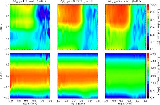
Contour plots for the polarization fraction (top row) and polarization angle (bottom row) as functions of the photon energy and cos θ for different values of the twist angle and the electron bulk velocity: |$\Delta \phi _\mathrm{N{\rm -}S}=1.3$| rad, β = 0.3 (left column); |$\Delta \phi _\mathrm{N{\rm -}S}=1.3$| rad, β = 0.5 (middle column); |$\Delta \phi _\mathrm{N{\rm -}S}=0.9$| rad, β = 0.5 (right column). In all runs, it is Bp = 5 × 10¹⁴ G and Tel = 10 keV.
The only energy-dependent effect of scatterings on the polarization angle is a small feature recognizable near the south magnetic pole, between ∼3 and 10 keV. This is also associated with the north–south asymmetry we have already mentioned (see again FD). As a proof of the fact that this feature is due to RCS, it tends to disappear for low β and becomes more evident for higher velocities. Finally, we checked that varying both Bp and Tel has a very little effect on ΠL and χpol.
In order to illustrate the effectiveness of polarimetric measurements in removing the degeneracy of the model, we performed a series of simulations for different values of |$\Delta \phi _\mathrm{N{\rm -}S}$| and β, in such a way to produce spectra which are very close to each other. Results are shown in Fig. 2, where the number of photons collected at infinity (left column), polarization fraction (middle column) and polarization angle (right column) are shown. Although the plots for the photon spectrum are almost undistinguishable in the two cases we report, ΠL and χpol are dramatically different. This actually proves that measurements of polarization in magnetar X-ray emission could be of key importance to probe the different geometries of the magnetosphere, in addition to spectral analysis, which alone cannot, however, suffice.
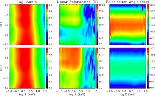
Contour plots for number of counts (in arbitrary units; left column), polarization fraction (middle column) and polarization angle (right column) as functions of the photon energy and cos θ for different values of the twist angle and the electron bulk velocity: |$\Delta \phi _\mathrm{N{\rm -}S}=1.3$| rad, β = 0.3 (top row) and |$\Delta \phi _\mathrm{N{\rm -}S}=0.7$| rad, β = 0.4 (bottom row). In all runs, it is Bp = 5 × 10¹⁴ G and Tel = 10 keV.
Phase-resolved simulations
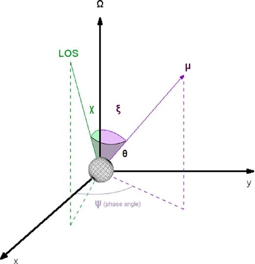
Geometry for phase-resolved simulations.
An example of a typical phase-resolved output is shown in the top row of Fig. 4, where the photon spectrum, polarization fraction and polarization angle as functions of energy and rotational phase are plotted for χ = ξ = 90°, corresponding to an orthogonal rotator seen perpendicularly to the spin axis. In this specific case, an observer can see all the surface, between the north (for ψ = 0, 2π) and the south (for ψ = π) magnetic poles.
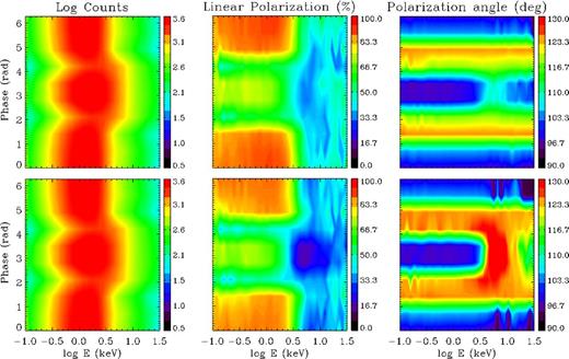
Number of counts (in arbitrary units; left column), polarization fraction (middle column) and polarization angle (right column) as functions of energy and rotational phase, for a simulation with Bp = 4.6 × 10¹⁴ G, |$\Delta \phi _\mathrm{N{\rm -}S}=1.3$| rad, β = 0.5 and Tel = 10 keV with (top row) and without (bottom row) QED effects. The star is assumed to be an orthogonal rotator seen perpendicularly to the spin axis (χ = ξ = 90°).
The polarization angle shows little dependence on the energy, as expected from the phase-averaged results, again apart from the feature localized near the south pole (i.e. around ψ = π in the present case) and between ∼3 and 10 keV, and due to the assumed unidirectional flow, as already discusses in Section 3.2. On the other hand, on varying the phase, χpol shows a maximum deviation from the initial value of 90° which occurs almost exactly at the magnetic equator (seen twice, at ψ = π/2 and 3π/2). Also the behaviour of the polarization fraction (top-middle panel) is rather similar to that of the phase-averaged simulations. However, again for the asymmetry caused by the choice of the unidirectional flow, in the ∼0.1–3 keV range the minimum value of ΠL occurs not in correspondence to the equator, as for the maximum value of χpol, but just a bit below (for ψ ∼ 2.1 and 4.2 rad). In fact, as noticed in Section 3.2, ΠL is quite sensitive to scattering, unlike χpol. This is the main reason for which the behaviour of the polarization angle is more symmetrical between the Northern and the Southern hemispheres than that of the polarization fraction, because the asymmetry is related only to scatterings.
Phase-resolved simulations allow us to clearly see the contribution of vacuum polarization effects (see Section 2.2), as compared to those of RCS. The bottom row of Fig. 4 shows again the number of counts, polarization fraction and polarization angle for the same values of the model parameters of the top row, but with the effects of QED turned off, so only RCS effects are accounted for. The photon spectrum is clearly the same, since it is not affected by vacuum polarization. The plots concerning the polarization observables are, instead, substantially different, the most evident result being that QED acts in smoothing out the polarization fraction and polarization angle behaviours. In particular, without QED effects, χpol (bottom-right panel) shows a sharp dependence on energy near the south magnetic pole where, as discussed above, RCS effects are more important. Also ΠL (bottom-middle panel) is affected by the absence of vacuum polarization, with an overall decrease of the polarization degree. Moreover, the phase values at which the maximum of the polarization angle and the minimum of the polarization fraction occur are closer to each other. So, in the absence of vacuum polarization, the polarization angle appears to be more sensitive to scatterings with respect to the complete QED+RCS situation discussed above.
OBSERVABILITY OF THE POLARIZATION SIGNATURES
In the previous sections, we have shown that polarimetry in X-rays can provide new observables for studying the magnetosphere and constraining the geometrical angles in magnetars. Here, we are going to investigate if, and to what extent, such observables can be measured by instruments which are likely be flown in the coming years on missions currently under development. To this end, we carried out detailed Monte Carlo simulations for evaluating the response of an exemplary polarimeter to the polarization signatures produced as radiation propagates through the magnetosphere. We first describe how we calculate the sensitivity of the instrument and then we present how we derive, from a Monte Carlo simulated measurement, the phase-resolved linear polarization degree and polarization angle.
Instrumental sensitivity
Current polarimeters for X-ray astronomy are based on the dependence of Bragg diffraction, photoelectric effect or Compton scattering on the linear polarization of the incident radiation since they can provide enough sensitivity for an astronomical measurement. On the other hand, X-ray magnetic circular dichroism and the dependence of Compton scattering on circular polarization have not been proven, as yet, of comparable efficiency; for this reason, and given the low degree of circular polarization expected in magnetars ( ≲ 5 per cent), in the following circular polarization will not be considered. We focus our discussion on the 2–6 keV energy range because the spectrum of magnetar sources peaks around a few keV's; here the polarization signatures are more evident and the measurement is easier to accomplish. Moreover, since AXPs/SGRs are relatively faint sources at least in quiescence, the use of an X-ray telescope is usually convenient and, in this energy range, conventional telescopes based on grazing incidence can be easily exploited.
In this X-ray range, the most promising polarimeters are those based on the photoelectric effect (Costa et al. 2001). They can measure the polarization of the beam together with its spectrum with a moderate energy resolution, of the order of 20 per cent at 6 keV, and with an accurate timing of the event, usually at the level of few microseconds (Bellazzini et al. 2006; Black et al. 2007). In addition to that, the gas pixel detector (GPD; Bellazzini et al. 2007; Bellazzini & Muleri 2010) can provide also very good imaging capabilities (Fabiani et al. 2013; Soffitta et al. 2013b), which are particularly useful for studying faint sources because this allows for a proper removal of the background. Therefore, we will discuss in the following the sensitivity of an instrument based on the GPD, which is however quite representative of this class of instruments.
The GPD has been presented as a focal plane detector in a number of mission proposals, together with small (Costa et al. 2010), medium (Tagliaferri et al. 2012) or large (Bellazzini et al. 2010) area telescopes. In the following, we will take as an example the small mission XIPE (Soffitta et al. 2013a), recently proposed to the European Space Agency in the context of a call for launch in 2017, to prove that even a mission with limited resources can be extremely useful in studying the magnetospheric environment of a magnetar. We use a Monte Carlo technique to derive the value of the polarization which would be measured by the instrument and its error. The code has been already described in detail (Dovčiak et al. 2011) and here we summarize only its most relevant features.
In general, polarization in X-rays is derived from the measured modulation curve, which is basically the histogram of the azimuthal response of the instrument. For example, the modulation curve for photoelectric polarimeters is the histogram of the azimuthal emission direction of the photoelectrons (Bellazzini & Spandre 2010). In the case of polarized photons, the modulation curve shows a cosine square modulation the phase of which is related to the polarization angle and coincides with it for photoelectric polarimeters. The amplitude of the modulation is proportional to the degree of polarization and to the modulation factor μ, which is the amplitude of the instrumental response to completely polarized photons.
The purpose of the Monte Carlo is to produce a number of ‘trial’ modulation curves in the energy range of interest, fit them with a cosine square function and derive for each trial an estimate of the polarization which would be measured from that modulation curve. The number of entries in the histogram is instead the number of collected events in the considered energy interval, obtained by multiplying the source spectrum by the collecting area of the telescope and by the instrument efficiency, using the response matrix of the instrument including its energy resolution. Each trial is affected by a different Poisson noise in the number of entries per azimuthal beam; systematic effects, proven to be lower than 1 per cent for the GPD (Bellazzini & Muleri 2010), are neglected. In defining the energy interval, the code takes into account the finite energy resolution of the instrument. The ‘measured’ angle and degree of polarization which are provided by the Monte Carlo are the values derived by a random trial, whereas their errors are the average values over all trials. The efficiency and the modulation factor of the GPD are discussed in detail in other papers to which the interested reader is referred for more information (Muleri et al. 2008, 2010), whereas the collecting area of XIPE is presented in Soffitta et al. (2013a).
Simulated polarization measurements
As discussed in Section 3, the polarization signature of magnetars depends on a number of parameters. Here we aim at investigating if X-ray polarimetry can be exploited to measure them and to which extent observations can discriminate between different cases. In the following, we make explicit reference to phase-resolved measurements, which are the most promising because, albeit a phase-averaged measurement integrates all the counts, its expected degree of polarization is smaller since the polarization angle swings across the rotational phases.
The sensitivity of the XIPE mission is evaluated using as a template the AXP 1RXS J170849.0−400910 (1RXS J1708 for short).6 The source period and period derivative are P ≃ 11 s and |$\dot{P}\simeq 1.9\times 10^{-11}\, {\rm ss}^{-1}$|, respectively, implying a dipole field of 4.6 × 10¹⁴ G. 1RXS J1708, one of the brightest known magnetars (Rea et al. 2005; Campana et al. 2007), is slightly variable, with a (unabsorbed) flux ranging between 21 and 35 × 10−12 erg cm−2 s−1 when restricted to the 2–6 keV band. The estimated source distance is ∼3.8 kpc (Durant & van Kerkwijk 2006) and we adopt the column density derived by Rea et al. (2005), NH = 1.48 × 1022 cm−2. Spectral fits to high-statistics XMM–Newton data of 1RXS J1708 with the xspec NTZ model (i.e. the same spectral model discussed in Section 2) have been presented in Zane et al. (2009). The best-fitting parameters are kT = 0.47 keV, β = 0.34 and |$\Delta \phi _\mathrm{N{\rm -}S}=0.49$|; the column density, NH = 1.45 × 1022 cm−2, is fully in agreement with that obtained by Rea et al. (2005). No estimate of the angles ξ and χ could be derived, since the NTZ model is angle averaged, nor it has been obtained by other means.
The study of magnetar sources with similar properties to 1RXS J1708 would be in the core science for a small mission dedicated to X-ray polarimetry like XIPE. Thus, we assume a total observation time of 1 Ms, which is completely reasonable for such a kind of mission. The simulated source photon spectrum is then generated, as discussed in Section 4.1, starting from the output of the Monte Carlo code (see Section 3.1) for a given set of parameters. In order to produce phase-resolved polarization observables, data are collected in nine, equally spaced phase bins. In the following, we present simulations obtained for a model with the same magnetospheric parameters as derived from the spectral fit of 1RXS J1708 (see above), together with a set of other test cases, obtained varying |$\Delta \phi _\mathrm{N{\rm -}S}$| and β. In all simulations, the magnetic field and the column density were held fixed at the values inferred for 1RXS J1708 and model spectra have been normalized in such a way to produce a flux comparable to that of 1RXS J1708 for the assumed distance of 3.8 kpc. The electron temperature is always set at Tel = 10 keV.
A first example is shown in Fig. 5, where the XIPE simulated data for kT = 0.47 keV, β = 0.34, |$\Delta \phi _\mathrm{N{\rm -}S}=0.49$|, χ = 60° and ξ = 30° are compared with the model. The three panels refer to the 2–6 keV pulse profile (top), linear polarization fraction (middle) and polarization angle (bottom). The filled circles with error bars show the XIPE measured quantities while the solid lines represent the models computed for the same parameter values and different values of ξ (the model from which the simulated data were derived is shown by the black curve). As a matter of fact, since the polarization angle is almost independent of the energy, we can derive the average degree of polarization of each model in the 2–6 keV energy range by simply weighting the phase-resolved polarization spectrum P(E, ψ) with the photon spectrum S(E, ψ), that is, |$P(\psi )_{\mathrm{2{\rm -}6\, keV}} = \int _\mathrm{2\, keV}^\mathrm{6\, keV} P(E,\psi ) S(E,\psi )\, \mathrm{d}E/\int _\mathrm{2\, keV}^\mathrm{6\, keV} S(E,\psi )\, \mathrm{d}E$|. Although this issue will be discussed in more detail later on, it is quite evident that a simultaneous fit of the degree and angle of polarization would allow us to derive unambiguously the value of ξ; additional information could be derived from the light curve that the instrument provides thanks to its very good timing properties. A similar result holds by keeping constant the angle ξ and letting χ free to vary.
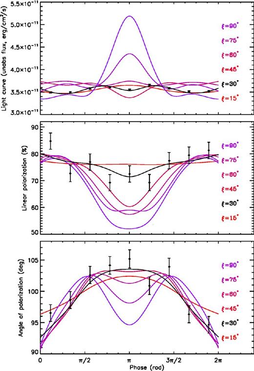
Pulse profile (top panel), phase-resolved polarization degree (middle panel) and polarization angle (bottom panel) for a set of models with the same viewing direction (χ = 60°) but with a different values of ξ. The filled circles denote the simulated data (with the associated 1σ errors) obtained with a 1 Ms observation of 1RXS J1708 by XIPE assuming χ = 60° and ξ = 30°. All quantities refer to the 2–6 keV energy range.
As a second example, which well illustrates the merits of X-ray polarimetry, we consider a case in which a different set of parameters produce an almost indistinguishable spectrum (this is the degeneracy which we already mentioned). The two models are shown in Fig. 6: one has |$\Delta \phi _\mathrm{N{\rm -}S}=0.7$| rad and β = 0.4 (solid line), and the other has |$\Delta \phi _\mathrm{N{\rm -}S}=1.3$| rad and β = 0.3 (dotted line); both models are for ξ = 60° and χ = 30°. The simulated XIPE data (filled circles with error bars) were generated from the former. As can be seen from the bottom panel, the unabsorbed spectra in the 2–6 keV range are almost identical, whereas a 1 Ms observation with XIPE clearly sets the two cases apart, both as far as the polarization degree and angle are concerned. It is worth noting that also a precise fitting of pulse profile allows us to discriminate the two models, and in fact this approach has been already put into practice (see, e.g., Albano et al. 2010). It is beyond the scope of this paper to determine whether polarimetry or phase-resolved photometry is more sensitive in measuring the magnetospheric parameters. Here we just say that the addition of these two new observables can be crucial for assessing the consistency of the model and, if so, to enhance the significance of the measurement.
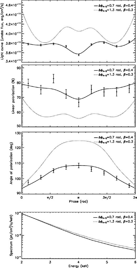
From top to bottom: comparison of the pulse profile, polarization degree, polarization angle and photon spectrum for two models characterized by |$\Delta \phi _\mathrm{N{\rm -}S}=0.7\mathrm{\ rad},\, \beta =0.4$| (solid line, model A) and |$\Delta \phi _\mathrm{N{\rm -}S}=1.3\mathrm{\ rad},\, \beta =0.3$| (dotted line, model B). The filled circles with error bars denote the simulated XIPE data obtained from model A. All quantities refer to the 2–6 keV energy range.
Finally, we discuss the capability of the method to recover the input model parameters from fitting the simulated data without any assumption, much in the same way as it would be done when confronting the model with ‘real’ observational data. To this end we exploit all the available observables, pulse profile, phase-dependent linear polarization fraction and angle, and perform a simultaneous fit leaving both the magnetospheric parameters (β, |$\Delta \phi _\mathrm{N{\rm -}S}$|) and the geometrical angles (χ, ξ) free to vary. The magnetic field strength, the surface and electron temperature together with the column density are, instead, held fixed at the values introduced previously and we refer here to the same case illustrated in Fig. 5, which is representative of 1RXS J1708. In this respect, we note that B can be estimated from the spin-down measure and both kT and NH from spectral fitting. Much in the same way as for the xspec NTZ model (see NTZ; Zane et al. 2009 for details), we produced beforehand a model archive covering the parameter ranges 0.2 ≤ β ≤ 0.7 (step 0.1), 0.3 ≤ ΔφN–S ≤ 1.4 rad (step 0.1), 15° ≤ χ ≤ 150° (step 15°) and 15° ≤ ξ ≤ 90° (step 15°). Single models were then loaded in an idl script which performs the fitting exploiting linear interpolation to obtain models for values of the parameters not included in the archive. We performed both simultaneous fits (pulse profile + polarization fraction + polarization angle) and individual fits to single observables. Results are shown in Fig. 7 and summarized in Table 1. The simultaneous fit of all the three observables is quite satisfactory (|$\chi ^2_\mathrm{red}=0.97$|) and returns parameter values which are well compatible with the input ones at the 2σ level. The only exception is the angle ξ, for which a value somewhat lower than the input one is derived (see again Table 1).
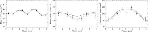
Simulated data (filled circles) and best simultaneous fit of the pulse profile, polarization degree and polarization angle in the 2–6 keV energy range (solid lines) for the same model as in Fig. 5 (β = 0.34, |$\Delta \phi _\mathrm{N{\rm -}S}=0.5\, \mathrm{rad}$|, χ = 60° and ξ = 30°). The dashed and dash–dotted lines show, respectively, the model from which data were generated and the individual fits.
Best-fitting parametersa.
| β | |$\Delta \phi _\mathrm{N{\rm -}S}$| | χ | ξ | |$\chi ^2_\mathrm{red}$| | |
|---|---|---|---|---|---|
| (rad) | (°) | (°) | |||
| Input values | 0.34 | 0.5 | 60 | 30 | – |
| 1RXS J1708 | 0.34 ± 0.004 | 0.51 ± 0.01 | 61.4 ± 0.9 | 25.7 ± 1.8 | 0.97 |
| Input values | 0.5 | 1.3 | 90 | 60 | – |
| QED-on | 0.501 ± 0.004 | 1.17 ± 0.03 | 90.3 ± 1.3 | 57.9 ± 2.2 | 1.17 |
| QED-off | 0.503 ± 0.002 | 1.34 ± 0.04 | 89.3 ± 1.4 | 60.4 ± 3.2 | 7.78 |
aReported errors are at the 1σ level.
We have seen that, at variance with the spectrum, the polarization signature is quite dependent on vacuum polarization. To better illustrate this, we computed two models for the same values of the parameters (χ = 90°, ξ = 60°, |$\Delta \phi _\mathrm{N{\rm -}S}=1.3$| rad and β = 0.5, similar to those of Fig. 4), the first with both scattering and vacuum polarization taken into account (‘QED-on’), whereas in the second vacuum polarization was turned off (‘QED-off’). We generated XIPE data from both simulations and attempted to fit the two sets using the model archive we introduced above and which includes vacuum polarization. Results are shown in Fig. 8, where the top panels refer to the ‘QED-on’ case and the bottom panels to the ‘QED-off’ one. While, as expected, the pulse profiles are indistinguishable, the polarization observables are quite different in the two cases, as can be seen from both the data points and the generating models (dashed lines). For ‘QED-on’, the simultaneous fit of the pulse profile, polarization fraction and angle is satisfactory (|$\chi ^2_\mathrm{red}\sim 1.2)$| and returns values compatible, within the errors, with the input ones (see Table 1). This, however, does not occur for the ‘QED-off’ data, to which ‘QED-on’ models provide an unacceptable representation (|$\chi ^2_\mathrm{red}\sim 7.8)$|. This shows that polarimetric measures are potentially capable of pinpointing QED effects in magnetar magnetospheres and can provide indirect evidence of an ultra-strong magnetic field.
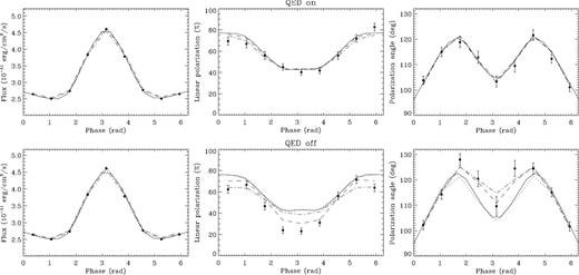
Comparison of the pulse profile, polarization degree and polarization angle (again in the 2–6 keV energy range) for two models both characterized by |$\Delta \phi _\mathrm{N{\rm -}S}=1.3\, \mathrm{rad}$|, β = 0.5, χ = 90° and ξ = 60°. The filled circles with error bars denote the XIPE data, generated with (top row) and without (bottom row) vacuum polarization. The solid and dash–dotted lines denote the simultaneous and individual fits, respectively, with ‘QED-on’ models. The dashed lines show the models from which data were produced, with (upper panels) and without (bottom panels) QED effects; in the bottom panels the model with vacuum polarization is also shown for comparison (dotted lines).
CONCLUSIONS
Previous investigations (FD; see also NTZ) have clearly indicated the potentialities of polarimetric measures at X-ray energies in probing the physics of magnetars. In this investigation, we have reconsidered the issue of polarization of X-ray radiation from magnetars within the framework of the twisted magnetosphere model, which has been successfully applied to reproduce the soft X-ray spectra of several magnetar candidates (SGRs/AXPs). While retaining some simplifications (globally twisted magnetosphere and unidirectional flow of charged particles along the closed field lines), our Monte Carlo simulations properly account for both the effects of RCS and of QED on the final polarization state of the emergent radiation.
Phase-averaged as well as phase-resolved results confirm that the linear polarization fraction ΠL and the polarization angle χpol are very sensitive to the magnetospheric twist angle |$\Delta \phi _\mathrm{N{\rm -}S}$| and the charge velocity β, and also to the geometric angles χ and ξ. This allows us to remove the |$\Delta \phi _\mathrm{N{\rm -}S}$|–β degeneracy which spectral measures alone cannot disambiguate. Polarization measurements can also univocally discriminate between the cases in which QED effects are present or not.
In order to assess the feasibility of magnetar X-ray polarization measurements, we simulated a 1 Ms observation of the bright AXP 1RXS J170849.0−400910 with XIPE, a small X-ray polarimetry mission recently proposed. We showed that it is indeed possible to extract the values of the physical and geometrical parameters from a phase-resolved measurement of polarization observables, by fitting the simulated data with a large set of our theoretical models. This more in-depth analysis also allows us to distinguish between different configurations in which photon spectra are very similar, therefore removing possible degeneracies. Finally, we proved that polarimetric measures are sensitive enough to reveal QED effects due to vacuum polarization, showing that polarization can be used as a tool to confirm the presence of ultra-strong magnetic fields in magnetars. Indeed, the sensitivity of state-of-the-art X-ray polarimeters appears today perfectly adequate to successfully probe the magnetospheric environment of a magnetar, ideally complementing spectral and timing measures and providing invaluable insight into the physical processes on the basis of ultra-magnetized NS.
We thank Silvia Zane and Enrico Costa for a number of useful comments on the manuscript. RT acknowledges financial support from an INAF PRIN 2011 grant.
Some transient magnetars exhibit a nearly thermal spectrum, modelled by one, or more, blackbody component(s) (e.g. Rea & Esposito 2011).
From the wave equation (8) it follows that Az = −(εzxAx/εzz + εzyAy/εzz). A non-vanishing Az implies that these are not plane waves. However, since it is |Az| ≪ |Ax| ∼ |Ay|, the amplitude of the oscillation along the propagation direction is vanishingly small and will be neglected hereafter.
In the presence of an inhomogeneous temperature distribution, radiation from the hotter patches has typically a larger polarization degree.
The circular polarization fraction is not considered here because it is not expected to be detectable with forthcoming X-ray instrumentation (see Section 4.1).
Also the azimuth ϕ changes with the phase, but this produces no effect because of the assumed symmetry around the magnetic axis.
See the McGill online magnetar catalogue at http://www.physics.mcgill.ca/pulsar/magnetar/main.html (Olausen & Kaspi 2013) and references therein.
