


Abstract
We present Hubble Space Telescope (HST) optical transmission spectra of the transiting hot-Jupiter WASP-12b, taken with the Space Telescope Imaging Spectrograph instrument. The resulting spectra cover the range 2900–10 300 Å which we combined with archival Wide Field Camera 3 spectra and Spitzer photometry to cover the full optical to infrared wavelength regions. With high spatial resolution, we are able to resolve WASP-12A's stellar companion in both our images and spectra, revealing that the companion is in fact a close binary M0V pair, with the three stars forming a triple-star configuration. We derive refined physical parameters of the WASP-12 system, including the orbital ephemeris, finding the exoplanet's density is ∼20 per cent lower than previously estimated. From the transmission spectra, we are able to decisively rule out prominent absorption by TiO in the exoplanet's atmosphere, as there are no signs of the molecule's characteristic broad features nor individual bandheads. Strong pressure-broadened Na and K absorption signatures are also excluded, as are significant metal-hydride features. We compare our combined broad-band spectrum to a wide variety of existing aerosol-free atmospheric models, though none are satisfactory fits. However, we do find that the full transmission spectrum can be described by models which include significant opacity from aerosols: including Rayleigh scattering, Mie scattering, tholin haze and settling dust profiles. The transmission spectrum follows an effective extinction cross-section with a power law of index α, with the slope of the transmission spectrum constraining the quantity αT = −3528 ± 660 K, where T is the atmospheric temperature. Rayleigh scattering (α = −4) is among the best-fitting models, though requires low terminator temperatures near 900 K. Sub-micron size aerosol particles can provide equally good fits to the entire transmission spectrum for a wide range of temperatures, and we explore corundum as a plausible dust aerosol. The presence of atmospheric aerosols also helps to explain the modestly bright albedo implied by Spitzer observations, as well as the near blackbody nature of the emission spectrum. Ti-bearing condensates on the cooler night-side is the most natural explanation for the overall lack of TiO signatures in WASP-12b, indicating the day/night cold trap is an important effect for very hot Jupiters. These findings indicate that aerosols can play a significant atmospheric role for the entire wide range of hot-Jupiter atmospheres, potentially affecting their overall spectrum and energy balance.
1 INTRODUCTION
Transit events have revolutionized our understanding of hot-Jupiter exoplanets, thanks in large part to atmospheric studies using transmission, emission and phase curve observations. Even with hundreds of known transiting hot Jupiters, currently only a small handful of exoplanets are capable of having their atmosphere characterized with all three types observations using current facilities, making these planets prototypes for the rest of the field. Among these planets is WASP-12b, a prototype ‘very hot Jupiter’ which is one of the largest and hottest planets known (Hebb et al. 2009). Extensive ground and space-based observations have been conducted on this planet over the last few years (Fossati et al. 2010, 2013; López-Morales et al. 2010; Campo et al. 2011; Chan et al. 2011; Croll et al. 2011; Maciejewski et al. 2011, 2013; Cowan et al. 2012; Crossfield et al. 2012b; Crossfield, Hansen & Barman 2012a; Haswell et al. 2012; Zhao et al. 2012; Copperwheat et al. 2013; Föhring et al. 2013; Stevenson et al. 2013; Swain et al. 2013).
As a very hot planet, most models predict strong Na, K, H2O and TiO/VO features in the atmosphere, with no condensates. WASP-12b has the potential to help address the stratospheric TiO hypothesis, which links the presence of TiO to thermal inversions (Fortney et al. 2008). As one of the largest planets, studying its atmosphere could also help gain insight into the connection between the anomalously large radius and atmospheric features.
Despite all the recent observations, the nature and composition of WASP-12b's lower atmosphere remains largely elusive, as both ground and space-based transmission spectra have not yet been able to place strong constraints on the presence of specific molecular features or atmospheric constituents (Copperwheat et al. 2013; Stevenson et al. 2013; Swain et al. 2013). Spectral retrieval methods on the day-side emission spectrum indicated that the planet contains a high C/O ratio (Madhusudhan et al. 2011), which would have important consequences regarding the planet's atmosphere (Madhusudhan 2012). However, WASP-12A is now known to have a close M-dwarf stellar companion discovered by Bergfors et al. (2011, 2013), which diluted previously reported transit and eclipse depths, especially in the infrared. After the diluting effects of the nearby M-dwarf have been taken into account, the day-side spectrum appears to largely resemble a blackbody (Crossfield et al. 2012b; Swain et al. 2013), which weakens the case for a high C/O ratio atmosphere.
Here, we present results from a large Hubble Space Telescope (HST) programme for WASP-12b (HST GO-12473; P.I. Sing), which is part of an eight planet optical atmospheric survey of transiting hot Jupiters, with the initial results given in Huitson et al. (2013) for WASP-19b and Wakeford et al. (2013); Nikolov et al. (2013) for HAT-P-1b. The overall programme goals are to detect atmospheric features across a wide range of hot-Jupiter atmospheres enabling comparative exoplanetology, detect stratosphere causing agents like TiO (Hubeny, Burrows & Sudarsky 2003; Fortney et al. 2008) and detect hazes and clouds. In this paper, we present new HST transit observations with the Space Telescope Imaging Spectrograph (STIS) instrument, and combine them with existing Wide Field Camera 3 (WFC3) spectra and Spitzer photometry to construct a high signal-to-noise (S/N) near-UV to infrared transmission spectrum, capable of detecting and scrutinizing atmospheric constituents. We describe our observations in Section 2, present the analysis of the transit light curves in Section 3, discuss the results in Section 4 and conclude in Section 5.
2 OBSERVATIONS
2.1 Hubble Space Telescope STIS spectroscopy
We observed two transits of WASP-12b with the HST STIS G430L grating during 2012 March 14 and 2012 March 27, as well as one transit with the STIS G750L during 2012 September 4. The G430L and G750L data sets all consist of 53 spectra, each spanning five spacecraft orbits. The G430L grating covers the wavelength range from 2900 to 5700 Å, with a resolution R of λ/Δλ = 530–1040 (∼2 pixels; 5.5 Å). The G750L grating covers the wavelength range from 5240 to 10 270 Å, with a resolution R of λ/Δλ = 530–1040 (∼2 pixels; 9.8 Å). Both the G430L and G750L data were taken with a wide 52 arcsec × 2 arcsec slit to minimize slit light losses. This observing technique has proven to produce high S/N spectra which are photometrically accurate near the Poisson limit during a transit event (e.g. Brown 2001; Sing et al. 2011; Huitson et al. 2012). The three visits of HST were scheduled such that the third and fourth spacecraft orbits would contain the transit, providing good coverage between second and third contact, as well as an out-of-transit (OOT) baseline time series before and after the transit. Exposure times of 279 s were used in conjunction with a 128-pixel wide sub-array, which reduces the readout time between exposures to 21 s, providing a 93 per cent overall duty cycle.
The data set was pipeline-reduced with the latest version of calstis and cleaned for cosmic ray detections with custom idl routines. Cosmic rays typically affect ∼5 per cent of the CCD pixels in a typical 279 s exposure and the STScI pipeline is generally insufficient in cleaning the images. Therefore, we adopted the strategy developed by Nikolov et al. (2013) to clean the images. The procedure is based on median-combining difference images to identify cosmic ray events, substituting the affected pixels, and those identified by calstis as ‘bad’, with flux values interpolated from the nearby point spread function (PSF). The mid-time of each exposure was converted into BJDTBD for use in the transit light curves (Eastman, Siverd & Gaudi 2010). As the G750L grating suffers from fringing effects red-ward of ∼7250 Å, we obtained contemporaneous fringe flats at the end of observing sequence, using them to defringe the science frame images (also see Nikolov et al. 2013).
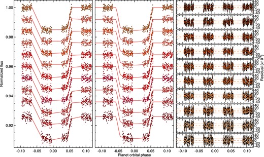
The spectral aperture extraction was done with iraf using a 13-pixel-wide aperture with no background subtraction, which minimizes the OOT standard deviation of the white-light curves. The extracted spectra were then Doppler corrected to a common rest frame through cross-correlation, which removed sub-pixel wavelength shifts in the dispersion direction. The STIS spectra were then used to create both a white-light photometric time series (see Fig. 1), and custom wavelength bands covering the spectra, integrating the appropriate wavelength flux from each exposure for different bandpasses. The resulting photometric light curves exhibit all the expected systematic instrumental effects taken during similar high S/N transit observations before HST Servicing Mission 4 with STIS, as first noted in Brown (2001).
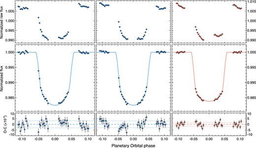
HST STIS normalized white-light curves for the three WASP-12b transits taken with the G430L (blue – left and middle) and G750L (red – right). Top panels: raw light curves normalized to the mean raw flux. The light curves experience prominent systematics associated primarily with the HST thermal-breathing cycle (see the text for details). Middle panels: detrended light curves along with the best-fitting limb-darkened transit model superimposed with continuous lines. Lower panels: observed minus modelled light-curve residuals, compared to a null (dashed lines) and 1σ level (dotted lines).
The main instrument-related systematic effect is primarily due to the well-known thermal breathing of HST, which warms and cools the telescope during the 96 min day/night orbital cycle, causing the focus to vary.1 Previous observations have shown that once the telescope is slewed to a new pointing position, it takes approximately one spacecraft orbit to thermally relax, which compromises the photometric stability of the first orbit of each HST visit. In addition for STIS, the first exposure of each spacecraft orbit has consistently been found to be significantly fainter than the remaining exposures. These trends are continued in our STIS observations and are both minimized in the analysis with proper HST visit scheduling. Similar to other studies, in our subsequent analysis of the transit we discarded the first orbit of each visit (purposely scheduled well before the transit event). In addition, we set the exposure time of the first exposure of each spacecraft orbit to be 1 s in duration, such that the exposure could be discarded without significant loss in observing time. We find that the second exposures taken for all five spacecraft orbits (each 279 s in duration) do not show the first-exposure systematic trend, making the short-exposure strategy an effective choice. However, we note that the first-exposure systematic in new observations of HD 189733 with the STIS G430L (GO 1306, P.I. Pont), persisted despite discarding similar 1 s initial exposures. As the HD 189733 time series exposures were much shorter (64 s), the 1 s strategy may only be effective for fainter targets like WASP-12, which have longer exposure times.
2.2 Hubble Space Telescope WFC3 spectroscopy
We also analyse the WFC3 G141 transit data of WASP-12 taken as part of GO 12230 (PI Swain), with results given in Swain et al. (2013). Our re-analysis is motivated by both a need for a consistently derived transmission spectrum with the STIS data, and the subsequent discovery of the M-dwarf companion (Bergfors et al. 2011, 2013) which affects the transit and eclipse depths (Crossfield et al. 2012b).
We use the flt outputs from WFC3's calwf3 pipeline. For each exposure calwf3 conducts the following processes: bad pixel flagging, reference pixel subtraction, zero-read subtraction, dark current subtraction, non-linearity correction, flat-field correction, as well as gain and photometric calibration. The resultant images are in units of electrons per second. The first orbit of the WFC3 data was removed, as it also suffers from thermal breathing systematic effects like STIS, leaving 391 exposures over the remaining four HST orbits, with a total of 175 exposures taken between first and fourth contact.
The spectra were extracted using custom idl routines similar to iraf's apall procedure, using an aperture of ±9 pixels from the central row, determined by minimizing the standard deviation across the aperture. The resulting 18 pixel wide aperture encompasses both WASP-12 and the M-dwarf binary. The aperture was traced around a computed centring profile, found to be consistent in the y-axis with an error of ±0.5 pixels. Background subtraction was applied using a region above and below the spectrum for each exposure. We elected to subtract the M-dwarf flux contribution through post-processing, though we note that nearly identical results can be obtained by instead excluding the M-dwarf flux using PSF fitting techniques (Swain et al. 2013).
For wavelength calibration, direct images were taken in the F132N narrow band filter at the beginning of the observations providing the absolute position of the target star. We assumed that all pixels in the same column have the same effective wavelength, with the extracted spectra covering the wavelength range of 1.077–1.704 μm.
2.3 Photometric monitoring for stellar activity
We also observed WASP-12 from the ground with Tennessee State University's automated Celestron C-14 telescope, located at Fairborn Observatory in southern Arizona. The telescope was equipped with an SBIG STL-1001E CCD camera observing through a Cousins R filter. Fig. 2 shows the Cousins R data for the 2011–2012 and 2012–2013 observing seasons plotted against Heliocentric Julian Date. The observations have been corrected for bias, flat-field, differential extinction, and pier-side offset. Differential magnitudes are computed against the mean of 17 comparison stars in the same CCD field. Each differential magnitude plotted is the mean of 8 to 10 successive frames on a given night. There are a total of 231 nightly observations, with transit points excluded from the plot. The standard deviation of an individual observation from the grand mean is 2.1 mmag. We find no significant periodicity between 1 h and 200 d in these data, with WASP-12A appearing quite constant. In particular, a least-squares sine fit of the C14 observations phased with the radial velocity period has a peak-to-peak amplitude of only 0.000 56 ± 0.000 41 mag, indicating little, if any, contribution to the radial velocity variations from stellar-surface activity. The late F spectral type of WASP-12 and its relatively low measured v sini (Knutson, Howard & Isaacson 2010), also makes it unlikely to have significant star spots, which is confirmed by our photometric monitoring. Alternatively, the low vsini could also be a result of a near pole-on view of the star as seen from the Earth, which is consistent with the spin-orbit misalignment measurement from Albrecht et al. (2012).
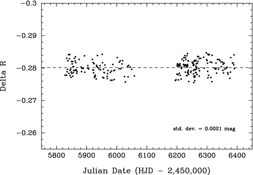
Stellar activity monitoring of WASP-12A from the Fairborn Observatory, showing the differential R magnitude from 2011 to 2013 with transits removed. The standard deviation of the light curve is 2.1 mmag, with no significant activity nor periodicity detected.
3 ANALYSIS
3.0.1 STIS white-light-curve fits
Our overall analysis methods are similar to the HST analysis of Sing et al. (2011); Huitson et al. (2013) and Nikolov et al. (2013), which we also describe briefly here. The light curves were modelled with the analytical transit models of Mandel & Agol (2002). For the white-light curves, the central transit time, inclination, stellar density, planet-to-star radius contrast, stellar baseline flux and instrument systematic trends were fit simultaneously, with flat priors assumed. The period was initially fixed to a literature value, before being updated, with our final fits adopting the value from Section 3.1. Both G430L transits were fitted with a common inclination, stellar density and planet-to-star radius contrast. The results from the G430L and G750L white-light-curve fits were then used in conjunction with literature results to refine the orbital ephemeris and overall planetary system properties (see Section 3.2). To account for the effects of limb darkening on the transit light curve, we adopted the four parameter non-linear limb-darkening law, calculating the coefficients with ATLAS stellar models (Teff = 6500, log g = 4.5, [Fe/H] = 0.0) following Sing (2010). Varying the stellar model within the known parameter range has a small effect on the output limb-darkening coefficients and fit transit parameters. In particular, we find changing the stellar effective temperature by ±250 K shifts the radius ratios by ∼1/3σ. Furthermore, the shift is typically common to all wavelength channels, and the relative radius ratio differences are largely preserved (to levels of ∼0.1σ in the case of WASP-12b).
As in many past STIS studies, we applied orbit-to-orbit flux corrections by fitting for a fourth-order polynomial to the photometric time series, phased on the HST orbital period. The systematic trends were fit simultaneously with the transit parameters in the fit. Higher order polynomial fits were not statistically justified, based upon the Bayesian information criteria (BIC; Schwarz 1978). The baseline flux level of each visit was let free to vary in time linearly, described by two fit parameters. In addition, similar to the STIS analysis of Sing et al. (2011); Huitson et al. (2012) and Huitson et al. (2013), we found it justified by the BIC to also linearly fit for two further systematic trends which correlated with the X and Y detector positions of the spectra, as determined from a linear spectral trace in iraf, as well as the wavelength shift between spectral exposures, measured by cross-correlation.
The errors on each data point were initially set to the pipeline values which is dominated by photon noise but also includes readout noise. The best-fitting parameters were determined simultaneously with a Levenberg–Marquardt least-squares algorithm (Markwardt 2009) using the unbinned data. After the initial fits, the uncertainties for each data point were rescaled based on the standard deviation of the residuals and any measured systematic errors correlated in time (‘red noise’), thus taking into account any underestimated errors in the data points. The red noise was measured by checking whether the binned residuals followed a N−1/2 relation, when binning in time by N points. In the presence of red noise, the variance can be modelled to follow a |$\sigma ^2=\sigma _{\rm w}^2/N+\sigma _{\rm r}^2$| relation, where σw is the uncorrelated white noise component, and σr characterizes the red noise (Pont, Zucker & Queloz 2006). We find that the pipeline per-exposure errors are accurate at small wavelength bin sizes, which are dominated by photon noise, but are in general an underestimation at larger bin sizes. For the STIS white-light curves, we find σr = 0.000 08 for the G430L and σr = 0 for the G750L. A few deviant points from each light curve were cut at the 3σ level in the residuals.
3.0.2 WFC3 white-light-curve fits
The noise properties and systematics of WFC3 G141 spectra are becoming fairly well understood, and are mainly affected by the HST thermal-breathing variation (note the similarities of Figs 1 and 3) and detector persistence which causes a ramp effect, also known as the ‘hook’ (Berta et al. 2012; Deming et al. 2013; Swain et al. 2013). These trends are predominantly either common-mode (i.e. the same in every wavelength channel across the detector) or repeatable orbit-to-orbit, and thus straightforward to remove in a variety of ways without affecting the relative transit depths (Berta et al. 2012; Deming et al. 2013; Huitson et al. 2013). The amplitude of the ‘hook’ has been studied as a function of exposure level, and reported in Deming et al. (2013). The authors found that the effect is practically zero when the exposure level per frame is lower than 30 000 electrons/pixel, which is also well within the linear regime of the detector. As the maximum count rates for the WASP-12 WFC3 data are in the range of 38 000 electrons/pixel, thus not substantially higher than the nominal lower threshold, no obvious ‘hook’ systematics are observed (see also Swain et al. 2013).

Similar to Fig. 1 but for the HST WFC3 transit.
We modelled the WFC3 white-light curve using the same analytic transit model and limb-darkening stellar model as used in the STIS analysis. Before the model fits, we subtracted the flux contribution from the M-dwarfs calculated from the WFC3 G141 response and the flux ratio as determined by Crossfield et al. (2012b), which matches well with our STIS analysis of both the M-dwarf spectral type and flux normalization (see Section 3.3). We excluded the ends of the spectrum, where the response drops rapidly, extracting the region from 1.137 to 1.657 μm to use for the white-light curve.
Like in the STIS analysis, the systematic effects of the thermal breathing were modelled with a fourth-order polynomial, phased on the HST orbital period, with the stellar baseline flux free to vary linearly in time. Unlike Swain et al. (2013), we find that higher orders in HST orbital phase are required to more fully remove the systematic errors. An alternative method has been developed by Berta et al. (2012) to correct for detector systematics, which takes advantage of the repetitive nature. Dubbed divide-OOT, the procedure involves creating a template baseline-flux time series for each subsequent exposure of an HST orbit, determined by averaging the OOT exposures. The light curve for each of the HST orbits are then divided by the OOT time series, which removes the systematic error components which are common to each orbit. We find divide-OOT gives very similar results as the parametrized method (as WFC3 exhibits largely common-mode systematics), though shows somewhat higher levels of correlated noise, as there are HST orbital phase mismatches between the sub-exposures of the five HST orbits, leading to residual thermal breathing trends which are evident in the residuals. We adopt the parametrized method both because of the somewhat lower noise values (σr = 0.000 04), and it is more straightforward to budget for the effects of the dominant thermal-breathing systematic on the transit depths through the use of the covariance matrix [or alternatively the Markov Chain Monte Carlo (MCMC) posterior distribution]. The M-dwarf flux contribution in the WFC3 is 7.16 ± 0.31 per cent, which translates to a systematic uncertainty on the radius ratio when subtracting the flux of 0.000 18 Rp/R*, which is small compared to our final WFC3 white-light-curve radius and uncertainly of 0.119 77 ± 0.000 42 Rp/R*.
In comparing our results to the literature, a source of disagreement is the overall Rp/R* level, which we find significantly higher than Stevenson et al. (2013), with our levels much closer to those of Swain et al. (2013). As noted by Stevenson et al. (2013), this is a result of the exponential function with time which they used to model the instrument systematics, which effectively ‘carves out’ the transit baseline flux leading to smaller fit radii. We see no evidence for a time-dependent exponential function (see Fig. 3), with our raw WFC3 white-light curve showing a closer resemblance to the STIS G750L data and its thermal-breathing trends.
3.1 Transit ephemeris
We used the central transit times of our HST data along with the transit times of Hebb et al. (2009), Chan et al. (2011), Maciejewski et al. (2011) and Cowan et al. (2012) to determine an updated transit ephemeris. When calculating transit ephemerides from data taken with different instruments in different wavelengths, it is important to use coherent and realistic estimates. Pont et al. (2006) showed how correlated noise could dominate the error budget of system parameter measurements from transit photometry. This issue is especially important for ground-based photometry of WASP-12, given that the M0 dwarf companions lie 1 arcsec from the target star, making very high precision photometry more difficult in changing seeing conditions. As the uncertainties given by Maciejewski et al. (2011) do not account for the effect of correlated noise, as a conservative estimate, we multiplied the error bars by a factor of 3, found to be typical for ground-based photometry of transiting planets (see also Barros et al. 2013).
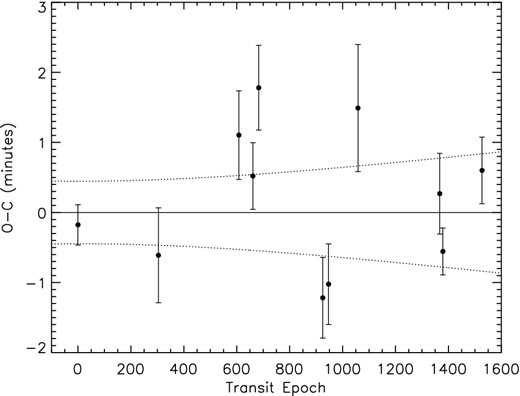
O−C diagram for the transit times of WASP-12 using the transits listed in Table 1 and a linear ephemeris. The 1σ error envelope on the ephemeris is plotted as the dotted lines.
Transit timing for WASP-12b.
| Epoc | BJDTBD | BJD error | Notes |
|---|---|---|---|
| 0 | 245 4508.976 88 | 0.000 20 | Hebb et al. (2009) |
| 304 | 245 4840.768 60 | 0.000 47 | Chan et al. (2011) |
| 608 | 245 5172.561 82 | 0.000 44 | Chan et al. (2011) |
| 661 | 245 5230.406 73 | 0.000 33 | Maciejewski et al. (2011) |
| 683 | 245 5254.418 87 | 0.000 42 | Maciejewski et al. (2011) |
| 925 | 245 5518.5407 | 0.0004 | Cowan et al. (2012) |
| 947 | 245 5542.5521 | 0.0004 | Cowan et al. (2012) |
| 1058 | 245 5663.701 59 | 0.000 63 | HST WFC3 |
| 1367 | 245 6000.949 87 | 0.000 40 | HSTG430L |
| 1379 | 245 6014.046 35 | 0.000 23 | HSTG430L |
| 1527 | 245 6175.577 48 | 0.000 33 | HSTG750L |
3.2 System parameters
The M-dwarf stellar companion is fully resolved with respect to the WASP-12 primary in our STIS spectroscopy. In combination with the high S/N, this permits a precise determination of the planetary radius completely free of the flux-dilution effects of the M-dwarf pair. Given that WASP-12b still has one of the largest radii of any transiting planet, a precise radius for this exoplanet, in particular, is crucial for understanding the hot-Jupiter inflation problem (see Baraffe, Chabrier & Barman 2010, for a review and the references therein).
We performed a joint fit of the two G430L white-light curves in conjunction with the radial velocity data from Hebb et al. (2009) and Husnoo et al. (2011). We used the MCMC suite EXOFAST from Eastman, Gaudi & Agol (2013) to perform the joint fit. In the joint fit, EXOFAST utilizes the Torres, Andersen & Giménez (2010) empirical polynomial relations between the masses and radii of stars, and their surface gravity, effective temperatures and metallicities. For the fit, we used priors on the orbital period and central transit time from Section 3.1 as well as priors on the stellar effective temperature, gravity and metallically from Hebb et al. (2009). In addition, in order to incorporate the information contained within the G750L and WFC3 light curves, we also put priors on a/R* and inclination based on the weighted-average transit fits to those data sets. The results are given in Table 2. In addition to finding updated parameters, the EXOFAST fits also serve to help verify the Levenberg–Marquardt transit fits and errors, with all of the fitted parameters and errors consistent at the 1σ level between the two methods, when similar fits are performed, including the values derived for the systematic error parameters described in Sections 3.0.1 and 3.0.2.
Best-fitting joint parameters for WASP-12.
| Parameter | Description | Value |
|---|---|---|
| Stellar parameters | ||
| M* | Mass (M⊙) | |$1.362_{-0.059}^{+0.060}$| |
| R* | Radius (R⊙) | |$1.602_{-0.035}^{+0.037}$| |
| ρ* | Density (cgs) | 0.467 ± 0.024 |
| log (g*)a | Surface gravity (cgs) | 4.162 ± 0.016 |
| Teffa | Effective temperature (K) | |$6400_{-180}^{+190}$| |
| [Fe/H]a | Metalicity | 0.159 ± 0.083 |
| Planetary parameters: | ||
| Pa | Period (d) | |$1.091\,421\,66_{-0.000\,000\,31}^{+0.000\,000\,32}$| |
| a | Semi-major axis (au) | |$0.023\,00_{-0.000\,34}^{+0.000\,33}$| |
| MP | Mass (MJ) | |$1.417_{-0.048}^{+0.049}$| |
| RP | Radius (RJ) | |$1.848_{-0.049}^{+0.052}$| |
| ρP | Density (cgs) | 0.279 ± 0.019 |
| log (gP) | Surface gravity | |$3.012_{-0.020}^{+0.019}$| |
| Teqb | Equilibrium Temp. (K) | |$2578_{-73}^{+75}$| |
| RV parameters: | ||
| K | RV semi-amplitude (m s−1) | |$225.8_{-3.9}^{+3.8}$| |
| MPsin i | Minimum mass (MJ) | |$1.406_{-0.047}^{+0.048}$| |
| MP/M* | Mass ratio | 0.000 994 ± 0.000 022 |
| γ | Systemic velocity (m s−1) | 13.5 ± 2.3 |
| Transit parameters: | ||
| RP/R* | Radius of planet | |$0.118\,52_{-0.000\,80}^{+0.000\,81}$| |
| a/R*a | Semimajor axis | |$3.087_{-0.053}^{+0.052}$| |
| ia | Inclination (°) | |$82.72_{-0.72}^{+0.71}$| |
| b | Impact Parameter | |$0.391_{-0.033}^{+0.032}$| |
| δ | Transit depth | 0.014 05 ± 0.000 19 |
| τ | Ingress/egress dur. (d) | |$0.015\,34_{-0.000\,56}^{+0.000\,62}$| |
| T14 | Total duration (d) | |$0.1213_{-0.0012}^{+0.0013}$| |
| u1 | Linear limb-darkening coeff. | |$0.551_{-0.028}^{+0.029}$| |
| u2 | Quad. limb-darkening coeff. | |$0.220_{-0.021}^{+0.020}$| |
aParameter makes use of priors, see Section 3.2 for details.
bTeq assumes zero albedo and a uniform planetary temperature.
Non-linear limb darkening coefficients calculated for the G430L (top), G750L (middle) and WFC3 G141 (bottom).
| λ(Å) | c1 | c2 | c3 | c4 |
|---|---|---|---|---|
| 2900–3800 | 0.2075 | 1.0926 | −0.4758 | 0.0337 |
| 3800–4300 | 0.2262 | 0.8330 | −0.1838 | −0.0118 |
| 4300–4800 | 0.5893 | −0.6147 | 1.5498 | −0.6692 |
| 4800–5240 | 0.3542 | 0.7815 | −0.4770 | 0.1080 |
| 5240–5700 | 0.3816 | 0.6909 | −0.3983 | 0.0828 |
| 5300–5800 | 0.3842 | 0.6811 | −0.3867 | 0.0783 |
| 5800–6300 | 0.4064 | 0.6433 | −0.4708 | 0.1154 |
| 6300–6800 | 0.4392 | 0.5138 | −0.3353 | 0.0538 |
| 6800–7300 | 0.4480 | 0.4646 | −0.2953 | 0.0460 |
| 7300–7900 | 0.4841 | 0.2891 | −0.1672 | 0.0023 |
| 7900–8500 | 0.4909 | 0.2526 | −0.1235 | −0.0147 |
| 8500–10 300 | 0.5009 | 0.1323 | −0.0197 | −0.0562 |
| 11 370–11 890 | 0.4552 | 0.2941 | −0.3676 | 0.1205 |
| 11 890–12 410 | 0.4275 | 0.4063 | −0.4985 | 0.1723 |
| 12 410–12 930 | 0.4622 | 0.3591 | −0.5380 | 0.2043 |
| 12 930–13 450 | 0.4319 | 0.4980 | −0.7316 | 0.2920 |
| 13 450–13 970 | 0.4654 | 0.4057 | −0.6303 | 0.2488 |
| 13 970–14 490 | 0.5023 | 0.4198 | −0.7869 | 0.3474 |
| 14 490–15 010 | 0.5156 | 0.3447 | −0.6864 | 0.3042 |
| 15 010–15 530 | 0.6272 | 0.1071 | −0.5256 | 0.2657 |
| 15 530–16 050 | 0.6514 | 0.0618 | −0.5024 | 0.2616 |
| 16 050–16 570 | 0.6756 | 0.0228 | −0.4738 | 0.2539 |
The resulting planetary radius is in general somewhat larger than past studies (Chan et al. 2011), expected as the M-dwarf serves to dilute the transit depth. With a joint fit using all of the available radial velocity data, our derived absolute radius is also nearly a factor of 2 more precise than recent ground-based studies (Maciejewski et al. 2013). Consequently, our derived bulk density of ρP = 0.279 ± 0.019 (cgs) for the planet is significantly lower than past studies (4.5σ compared to Chan et al. 2011), further adding to the confirmation of an anomalously large radius for this planet.
3.3 M-dwarf stellar companions
The M-dwarf companion is well resolved in both the STIS acquisition images (see Fig. 5) and in the STIS spectra. This provides an opportunity to further characterize the properties of the M-dwarf, and its impact on the WASP-12 system. Crossfield et al. (2012b) found that the M-dwarf was consistent with a spectral type of M0V, with an effective temperature of Teff = 3660 K using near-IR spectroscopy. In addition, they found that the system may possibly be associated with WASP-12A if the M-dwarf was found to be a close binary pair, but with only low-resolution images at the time, they could not firmly conclude its association. However, they did note that the ground-based images had an extended PSF profile and that the two objects had a common system radial velocity, pointing towards a binary M-dwarf pair.

HST STIS optical acquisition image of WASP-12A and the two faint M-dwarf companions located 1.06 arcsec to the south-west of the transit hosting star. Shown is the image (left) on a logarithmic flux scale to illustrate the PSF of WASP-12A and (right) on a linear flux scale set to maximize the contrast of the north–south aligned M-dwarf pair.
In order to align the HST PSF within the STIS long slit, an optical broad-band acquisition image was initially taken with the F28×50LP filter, which has a wavelength range between 5490 and 9990 Å and a central wavelength of 7150 Å. With HST's high resolution, these images immediately reveal the M-dwarf to be a binary pair (see Fig. 5), confirming the suspicions of Crossfield et al. (2012b) and Bergfors et al. (2013). Furthermore, the two components of the M-dwarf binary are observed to have equal brightness, implying equal mass, with a flux contrast between the two estimated from the central pixel intensities to be 1.08±0.07 from the acquisition image. The near unity flux contrast between the two stars also matches the recent ground-based adaptive optics imaging results of Bechter et al. (2013).
Being spatially well resolved from WASP-12A in STIS spectral images, we also extracted the optical spectrum of the M-dwarf companions (see Fig. 6). The STIS G750L spectrum of the M-dwarf pair matches very well with the Teff = 3660 K measurement of Crossfield et al. (2012b), lending further evidence of the two stars possessing the same spectral classification, with the spectral typing of the combined pair consistent between the two studies from the optical to K band.

HST STIS G750L spectrum of the M-dwarf binary pair (black) compared to main-sequence library stellar spectra taken from Pickles (1998) with Teff of 3800 (top blue), 3680 (middle green) and 3550 (red bottom). All spectra are normalized in flux at 5500 Å. The best matching 3680 K spectrum is consistent with the results of Crossfield et al. (2012b), who determined a Teff of 3660|$^{+85}_{-60}$| K corresponding to an M0V dwarf. The STIS spectrum red-ward of about 7250 Å is affected by detector fringing, causing the observed deviations from the best-fitting template spectrum.
Compared to WASP-12A, the flux contrast between the two M-dwarf stars and the WASP-12A primary is 0.0207 ± 0.0004 in the HST image, which is close to the Δi′ measurement of Bergfors et al. (2013). Assuming an equal-mass M-dwarf binary, the distance modulus from Crossfield et al. (2012b) is re-evaluated to be 7.85 ± 0.2 mag for the M-dwarfs which compares to 7.7 ± 0.2 mag for WASP-12A, placing the three stars at the same distance (within the errors), making a triple-star configuration highly likely. At a distance of 427 pc (Chan et al. 2011), the projected separation between WASP-12A and the M-dwarfs is 450 au, and the M-dwarf binary projected separation is about 40 au. A final proof of association would be a common proper motion measurement between the three stars (see Bechter et al. 2013).
3.4 Transmission spectrum fits
We extracted various wavelength bins2 for the STIS G430L, G750L and WFC3 G141 spectra, to create a broad-band transmission spectrum and search for expected narrow band features (see Figs 7, 8 and 9). In these transit fits, we fixed the transit ephemeris to the results from Section 3.1 and fixed the inclination and stellar density to their best-fitting values, allowing RP/R* to be free as well as the baseline flux and model parameters describing the instrument systematic trends. The WFC3 spectra were M-dwarf flux corrected in the same manner as the white-light curve (see Section 3.0.2), with the uncertainty from the correction well under each of our 1σ errors for Rp/R*.

HST STIS G430L spectral bin transit light curves jointly fit for visit 1 (top) and visit 2 (bottom). (Left) Light curves for the HST STIS G430L spectral bins with the common-mode trends removed, overplotted with the best-fitting systematics model. The points have been offset in relative flux, and systematics model plotted with connecting lines for clarity purposes. The light curves are ordered in wavelength, with the shortest wavelength bin shown at the top and longest wavelength bin at the bottom. (Middle) Light curves fully corrected for systematic errors, with the best-fitting joint transit model overplotted. (Right) Residuals plotted with 1σ error bars along with the standard deviation (dotted lines).
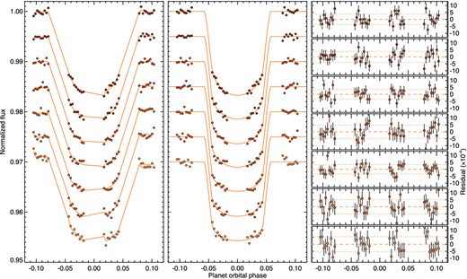
The same as Fig. 7, but for the G750L spectral bins.
The limb-darkening parameters were fixed to the model values, with the four non-linear coefficients for each bin individually calculated from the stellar model, taking into account the instrument response (see Table 3). As a separate direct test of the limb-darkening model used, we fit a light curve with a free limb darkening coefficient in a spectral bin between 4000 and 4500 Å using a linear law, and compared the fit coefficient u to the stellar model prediction. At these wavelengths, the predicted limb darkening is approximately linear (with a linear law deviating from ATLAS stellar model intensities by no more than 3.2 per cent, except at the very limb), making a direct comparison of the stellar model and transit-fit limb-darkening coefficients straightforward.3 The fitted linear coefficient is very close to the stellar model value, with a simultaneous fit of the two G430L transits resulting in u = 0.772 ± 0.023 which compares favourably to the ATLAS model prediction of 0.774. Furthermore, we note that our transmission spectrum did not substantially change when fitting the light curves using a linear limb-darkening law with a freely fit coefficient, and the BIC favoured fixing the limb-darkening parameters to the model values.
We handled the modelling of systematic errors in the spectral bins by two methods. In the first method, we allowed each light curve to be fit independently with a parametrized model, as done in the white-light-curve analysis. In the second method, we removed the common-mode trends from each spectral bin before fitting for the residual trends, again with a parametrized model but fitted with fewer parameters. The common-mode trends were extracted from the white-light curves, by removing the transits from the raw light curves using the parameters derived from the best-fitting models. These common-mode trends were then removed from each spectral bin, normalized to preserve the overall flux levels. In particular, removing the common trends reduces the amplitude of the breathing systematics by a considerable margin, as these trends are observed to be very similar wavelength-to-wavelength across the detector.
As found in Nikolov et al. (2013) for the HAT-P-1b STIS transit data, we find that it makes little difference (i.e. deviations of ∼1σ or less on the fitted RP/R* values) whether to include or not the position-related trends when fitting for the transit depths, as compared to optimizing the systematic trends for each bin individually based on the BIC. In the fully parametrized method, we elected to fit the same model as used for the white-light curve (fourth order in HST phase and linear in X-position, Y-position, time and wavelength shift) as a some of the bins did prefer the model, and a uniform model for all wavelength channels helps ensure that residual instrument trends are not differing channel-to-channel, adversely affecting the transit depths. With this method, we reach average precisions of 73 per cent the photon noise limit with the G430L, and 87 per cent for the G750L, with no significant red noise detected.
In the common-mode analysis, the spectral bins for the two G430L transits were each fitted with three fewer parameters compared to the fully-parametrized method, as the third- and fourth-order HST phase trends as well as the linear slope did not justify being fit. Similarly, for the G750L spectral bins, the four orders of the HST phase trend polynomial and wavelength shift trend did not need to be fit, reducing the number of nuisance parameters for each light curve from 8 to 3. In addition, the common-mode analysis typically performed comparable or better than the full-parametrized model, with the G430L attaining an average precisions of 80 per cent the photon noise limit, and the G750L attaining 85 per cent the photon noise limit. The biggest improvement is seen where the grating efficiencies are low, as the spectral bins with lower counts are more dominated by photon noise, making it harder for a parametrized model to accurately fit for low-level systematic trends.
As done with STIS, we also fit the WFC3 spectral bins using a fully parametrized model and a common-mode removal analysis. As with the STIS data, the common-mode trends derived from the WFC3 white-light curve dramatically reduced the apparent trends in the spectral bins. We report bin sizes which are comparable to the STIS data, 560 Å wide, which is courser resolution than reported in Swain et al. (2013) as no obvious spectral features were apparent at higher resolution.
For the common-mode analysis, the number of nuisance parameters was reduced from 5 to 2, with a quadratic function of HST phase used to fit the residual trends. With the fully parametrized method, the precisions attained are close to those of Swain et al. (2013) who reported typical precisions near ∼86 per cent the photon noise limit. The common-mode analysis performed better, with an improvement of about 4 per cent in the residual scatter of the binned light curves with the common-mode method. For both reduction methods, when binning the data similarly as the two aforementioned studies, we find nearly identical transmission spectral results. The one notable exception is the shortest wavelength channel of Swain et al. (2013) which is more than 2σ higher than our results. With the common-mode analysis, we also find that binning the spectra to wider bandpasses does not significantly degrade the performance relative to the photon limit, as found by Swain et al. (2013) who adopted a linear analysis.
Given the overall better performance with significantly fewer nuisance parameters, we adopt the common-mode analysis for further study, though note that all of the subsequent results would be nearly identical if instead we adopted the fully parametrized analysis for both the STIS and WFC3 spectra. The broad-band spectral results are given in Table 4 and shown in Fig. 10, where we have included the Spitzer transit photometry of Cowan et al. (2012) as re-evaluated with the M-dwarf dilution correction by Crossfield et al. (2012b). We have chosen the non-prolate value for the 4.5 μm transit depth measurement of Cowan et al. (2012), which is consistent with the WFC3 eclipse photometry of Swain et al. (2013).
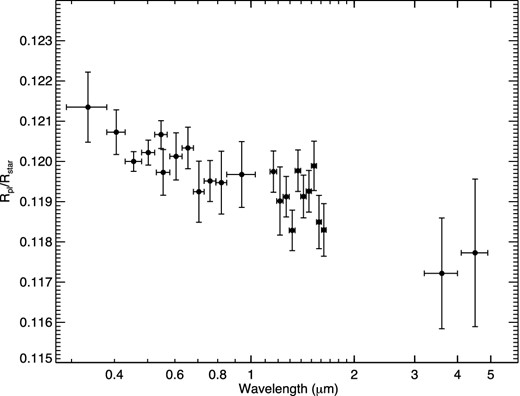
Combined HST STIS, HST WFC3 and Spitzer transmission spectrum of WASP-12b.
Broadband transmission spectral results for WASP-12b for the G430L (top), G750L (middle) and WFC3 G141 (bottom).
| λ(Å) | RP/R* |
|---|---|
| 2900–3800 | 0.121 35 ± 0.000 87 |
| 3800–4300 | 0.120 73 ± 0.000 56 |
| 4300–4800 | 0.120 00 ± 0.000 25 |
| 4800–5240 | 0.120 22 ± 0.000 31 |
| 5240–5700 | 0.120 67 ± 0.000 35 |
| 5300–5800 | 0.119 73 ± 0.000 57 |
| 5800–6300 | 0.120 12 ± 0.000 59 |
| 6300–6800 | 0.120 33 ± 0.000 51 |
| 6800–7300 | 0.119 25 ± 0.000 76 |
| 7300–7900 | 0.119 51 ± 0.000 51 |
| 7900–8500 | 0.119 47 ± 0.000 78 |
| 8500–10 300 | 0.119 67 ± 0.000 82 |
| 11 370–11 890 | 0.119 75 ± 0.000 51 |
| 11 890–12 410 | 0.119 02 ± 0.000 85 |
| 12 410–12 930 | 0.119 12 ± 0.000 50 |
| 12 930–13 450 | 0.118 29 ± 0.000 50 |
| 13 450–13 970 | 0.119 77 ± 0.000 52 |
| 13 970–14 490 | 0.119 13 ± 0.000 53 |
| 14 490–15 010 | 0.119 26 ± 0.000 52 |
| 15 010–15 530 | 0.119 89 ± 0.000 61 |
| 15 530–16 050 | 0.118 49 ± 0.000 66 |
| 16 050–16 570 | 0.118 30 ± 0.000 65 |
| 36 000 | 0.117 22 ± 0.001 38 |
| 45 000 | 0.117 73 ± 0.001 83 |
4 DISCUSSION
4.1 Searching for narrow band spectral features
In addition to deriving the broad-band spectrum, we searched the STIS data for narrow band absorption signatures, including the expected species of Na, K, Hα and Hβ, as the line cores of these elements can have strong signatures. In the context of the HST survey, Na has been detected in Hat-P-1b by Nikolov et al. (2013), who found the strongest signal in a 30 Å bandpass around the Na doublet.
We find no evidence for Na, either in wide or medium-size bandpasses. In a 30 Å wide medium bandpass, we measure a planet-to-star radius difference of ΔRp/R* = (− 0.3 ± 2.0) × 10−3 compared to a 600 Å wide reference region encompassing the Na doublet. Theoretical models which are assumed to be dominated by Na absorption in this region predict features of 4.0× 10⁻³ ΔRp/R*, so the data can rule out significant Na absorption with about 95 per cent confidence. Any Na feature present in WASP-12b must be confined to a narrow core, similar to HD 189733b or XO-2b (Huitson et al. 2012; Sing et al. 2012).
Similar to Na, we also find no evidence for Hα, Hβ, nor K. A 75 Å wide bandpass centred on the K doublet gives a radius difference of ΔRp/R* = (− 2.6 ± 1.9) × 10−3.
4.2 A thorough search for TiO
As one of the most highly irradiated hot Jupiters discovered to date with a zero-albedo equilibrium temperature of Teq = 2580 K, WASP-12b is a prime target to search for signatures of TiO. TiO has strong opacity throughout the optical, with one of the strongest signatures being a ‘blue edge’ at the short-wavelength end (∼4300 Å) of the molecule's optical bandheads, making the STIS G430L an ideal instrument to detect the species. Without the optical-blue wavelengths of STIS, ruling out TiO in the atmosphere is not so straightforward. For one, the required optical-blue precisions are difficult to obtain from the ground (Copperwheat et al. 2013). In addition, the overall higher planetary radius levels as seen in the optical-red compared to the near-IR can be reasonably well matched by models which include TiO, especially if the model abundances and temperature profiles are fit (Stevenson et al. 2013).
Our broad-band transmission spectrum shows no signs of TiO. In particular, while models expect the radius to drop by 2.4 × 10⁻³Rp/R* blueward of 4300 Å, our measured radii instead increase by an average of (0.9 ± 0.5) × 10−3Rp/R* compared to the 4300–4800 Å bin, representing a 6.6σ confident non-detection of TiO at the ‘blue-edge’. Radiative transfer models assuming equilibrium chemistry and solar compositions have strong TiO features, and offer overall unsatisfactory fits to the broad-band data, with a Fortney et al. (2010) model giving a χ2 of 44 for 23 d.o.f. (see Fig. 11).

As our broad-band spectrum is not optimally configured to detect individual TiO bandheads, we employed custom-tailored bins following the TiO ‘comb’ approach of Huitson et al. (2013) which sub-divides the region between 4840 and 7046 Å into two optimal bandpasses. An ‘in’ bandpass specifically covers wavelengths of eight strong TiO bandheads, while an ‘out’ bandpass covers the wavelength regions between the bandheads. A positive TiO detection would show up as an increased radius in the ‘in’ bandpass compared to the ‘out’, and a positive [TiO]comb value. In this manner, we are able to use a very large portion of the STIS data to search for specific TiO features, providing good sensitivity. This search also rules out TiO, with the G430L and G750L giving an average [TiO]comb radius difference of ΔRp/R* = (− 0.51 ± 0.42) × 10−3 while WASP-12b models with TiO predict a difference of +0.82× 10⁻³Rp/R*, representing a 3.2σ confident non-detection of molecular bandheads.
As done in Huitson et al. (2013), we also searched for the distinct ‘red edge’ at 7396 Å, where the broad-band opacity of TiO drops significantly towards longer wavelengths. No significant difference in altitude was found with a ΔRp/R* measured to be [TiO]red = (−0.87 ± 0.71) × 10−3 between an ‘in’ band from 6616 to 7396 Å and an ‘out’ band between 7396 and 8175 Å, while models predict a difference of +1.4× 10⁻³Rp/R*, a 3.2σ confident non-detection of the ‘red edge’.
With three independent tests to search for the molecule giving sensitive null results, significant TiO absorption is decisively ruled out at high confidence as there are no spectral signs of the characteristic ‘blue-edge’, ‘red-edge’, nor its strongest optical bandheads. Similar to Na or K, any TiO absorption features in the transmission spectrum of WASP-12b must be confined to narrow band signatures of the molecule's strongest optical transitions.
4.3 A search for metal hydrides
Metal hydrides, including TiH and CrH, have been suggested and explored as possible opacity sources in WASP-12b when modelling the red-optical and near-IR data (Stevenson et al. 2013; Swain et al. 2013), with TiH a potentially important Ti-bearing molecule in high C/O ratio atmospheres (Madhusudhan 2012; Stevenson et al. 2013). A complete optical spectrum in this regard helps constrain the presence of metal hydrides. In particular, as TiH has its strongest bandhead near 5300 Å (Sharp & Burrows 2007), the G430L is very sensitive to its presence.
We find no evidence for TiH, with narrower bandpasses around 5300 Å all consistent with the broad-band level near 0.1207 Rp/R*. The lack of the strong 5300 Å TiH bandhead constrains the presence other longer wavelength bandhead features of TiH to be at or below the observed optical and near-IR radius. Thus, we conclude TiH cannot be a major broad-band opacity source for the transmission spectra. The same is true for MgH, which also has its strongest peak in the optical-blue (Sharp & Burrows 2007), which we also do not observe.
Significant opacity by CrH can also be excluded, as abundances needed to match the WFC3 near-IR Rp/R* levels would produce strong features between 8000 and 10 000 Å which would rise to ∼0.122 Rp/R*, where the opacity of CrH is strongest (Sharp & Burrows 2007), though no such features are apparent.
In addition to these molecule-specific searches, we also explored a range of different atmospheric models with varying opacity (0.1 to 10 solar) as calculated in Burrows et al. (2010). These models contained significant metal hydride features (including MgH, FeH and CaH), though none were satisfactory fits to the broad-band data (see Table 5).
4.4 Limits on molecular absorption
Despite different reduction techniques and instrument systematic models, the shape of our near-IR transmission spectra agrees very well with other studies (Stevenson et al. 2013; Swain et al. 2013). The data are of sufficient quality to have detected H2O, if it were present at the levels some models predict, with the WFC3 atmospheric H2O detections in WASP-19b and HAT-P-1b a direct example (Huitson et al. 2013; Wakeford et al. 2013). In agreement with the findings of Swain et al. (2013), we find no strong evidence for H2O absorption, though there is a small ‘bump’ at 1.4 μm which is compatible with a small amplitude H2O feature. A straight-line (with two free parameters fit in Rp(λ)/R* versus lnλ) remains a good fit to the WFC3 data (χ2 = 9 for 8 d.o.f.).
A small amplitude H2O feature would imply that either the scaleheight is smaller than expected (requiring lower temperatures), the H2O abundance is low, or that the feature is being covered by other absorbers (including hazes or clouds, also see Section 4.5.4) as has been suggested for HD 209458b (Deming et al. 2013). We find that the WASP-12b WFC3 transmission spectrum is compatible with H2O-only absorption if the temperature is below 1600 K at 95 per cent confidence. This temperature presents a problem when interpreting the overall broad-band spectrum, as smaller scaleheights from lower temperatures would lead to a flatter overall spectrum, yet significant broad-band radii differences are observed. In addition, as pointed out by Stevenson et al. (2013), the Spitzer data is compatible with smaller radii, even though models with significant H2O (and CO) absorption predict larger radii at those longer wavelengths.
Potentially, HCN could be an important molecule in the atmosphere, especially if WASP-12b were to have a high C/O ratio (Bilger, Rimmer & Helling 2013; Moses et al. 2013). However, the cross-section of HCN is considerably weaker in the optical and near-IR compared to Spitzer wavelengths (e.g. see Shabram et al. 2011), which places constraints in our broad-band spectrum. As found by Stevenson et al. (2013), the near-IR and SpitzerRp/R* radius levels long-wards of 1.55 μm can reasonably reproduced assuming HCN dominates that region, but with a sharp drop in the opacity short-ward of 1.55 μm, our optical data and the near-IR WFC3 up to that wavelength would need an additional opacity source to explain the larger radius levels. While Stevenson et al. (2013) attributes the higher optical levels in part to TiO or TiH, both molecules are inconsistent with our blue-optical data. With current data, a re-analysis of the secondary eclipse data, taking into account the M0V dilution effects, would likely place stronger overall constraints on the presence of HCN than our transmission spectra.
We compared our broad-band spectrum to a variety of different clear atmospheric models (dominated by gaseous molecular and atomic features) from the 1D modelling suites of Burrows et al. (2010); Howe & Burrows (2012) and Fortney et al. (2008, 2010). The models include T − P profiles assumed to be isothermal, as well as day-side and planet-wide average profiles in radiative hydrostatic equilibrium. Models were also computed with a variety of different metalicities, C/O ratios, and heat redistribution efficiency parameters as well as extra optical absorbers used by Burrows et al. (2007) to produce stratospheres and interpret Spitzer secondary eclipse data. Models were also run with and without including gaseous TiO and with/without including metal hydrides. As shown in Table 5, none of the models are particularly good fits to the transmission spectrum data (see Fig. 12).
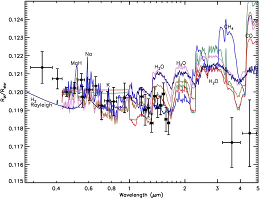
Plotted is the broad-band transmission spectral data compared to six different clear atmosphere models (which lack TiO) listed in Table 5, including Burrows-ExtraAbsorber_10×solar (red), Burrows-MetalHydrides_0.01×H2O (light blue), Burrows-ExtraAbsorber_10×CO (green), Burrows-Isothermal3000_0.1×solar (brown), Burrows-Isothermal2500 (orchid) and Fortney-Isothermal2250_noTiO (dark blue). All of these models have a particularly hard time simultaneously fitting for the near-IR WFC3 and Spitzer data.
Model selection fit statistics against the N = 24 broad-band transmission spectrum data points. Atmospheric models including aerosols are listed at the top, while clear atmospheric models (dominated by gaseous molecular and atomic absorption features) are listed at the bottom. The ΔBIC and relative probability for all models is calculated with respect to the Rayleigh scattering model. The Burrows et al. (2010) models are compared against the 22 longest wavelength data points, while the Fortney et al. (2010) models and are compared against all 24 points.
| Models (with aerosols) | χ2 | N, d.o.f. | BIC | D = ΔBIC/2 | Prob = exp(D) |
|---|---|---|---|---|---|
| Rayleigh scattering | 16.8 | 24, 22 | 23.1 | 0 | 1 |
| Mie scattering Al2O3 | 16.8 | 24, 22 | 23.1 | 0 | 1 |
| Titan tholin | 20 | 24, 22 | 26.4 | −1.7 | 0.19 |
| Settling Dust (β = −3) | 21.5 | 24, 22 | 27.9 | −2.4 | 0.09 |
| Mie scattering CaTiO3 | 24.0 | 24, 22 | 30.3 | −3.6 | 0.03 |
| Mie scattering Fe2O3 | 24.8 | 24, 22 | 31.2 | −4.0 | 0.02 |
| Settling Dust (β = 0) | 29.3 | 24, 22 | 35.7 | −6.3 | 0.002 |
| Fortney-noTiO_EnhancedRayleigh | 31.6 | 24, 22 | 40 | −7.4 | 0.0006 |
| Fortney-noTiO_CloudDeck | 47.4 | 24, 22 | 54 | −15 | 10−7 |
| Models (clear atmospheres) | χ2 | N, d.o.f. | BIC | D = ΔBIC/2 | Prob = exp(D) |
| Burrows-ExtraAbsorber_10×solar | 28.5 | 22, 20 | 34.7 | −6.3 | 0.0018 |
| Burrows-MetalHydrides_0.01×H2O | 39 | 22, 21 | 45 | −12 | 10−5 |
| Burrows-ExtraAbsorber_10×CO | 35 | 22, 19 | 44 | −11 | 10−5 |
| Fortney-Isothermal2250_withTiO | 44 | 24, 23 | 48 | −12 | 10−5 |
| Burrows-Isothermal3000_0.1×solar | 54 | 22, 20 | 60 | −19 | 10−8 |
| Burrows-withTiO | 58 | 22, 21 | 61 | −19 | 10−9 |
| Burrows-Isothermal2500 | 115 | 22, 21 | 118 | −48 | 10−21 |
| Fortney-Isothermal2250_noTiO | 134 | 24, 23 | 137 | −57 | 10−25 |
4.5 Interpreting the broad-band transmission spectrum with aerosols
While most of the expected molecular and atomic features can be confidently ruled out (e.g. TiO, Na and K) as major contributors to our broad-band transmission spectrum, the overall slope of the spectrum shows a significant broad-band atmospheric feature, with an overall characteristic slope which spans 0.0031Rp/R* from the optical to the infrared (see Fig. 10). The atmospheric pressure scaleheight H is given by |$H = \frac{kT}{\mu g}$|, where k is Boltzmann's constant, T is the local gas temperature, μ is the mean molecular weight of the atmosphere and g is the surface gravity. For WASP-12b, the scaleheight is estimated to be 700 km at 2100 K, implying that our broad-band transmission spectrum spans ∼5H in altitude (3500 km).
Assuming a temperature mid-way between the day-side and night-side temperatures of 3000 and 1100 K, respectively4 and allowing a temperature range which encompasses a Teq of 2578 K, gives a temperature in the range of 2100 ± 500 K. With these adopted temperatures, the slope of the transmission spectrum would imply an effective extinction cross-section of σ = σ(λ/λ0)−1.7±0.5.
4.5.1 Rayleigh scattering
Assuming that the atmosphere can be described by Rayleigh scattering (α = −4), as would be the case in a pure H2 atmosphere or one for an atmosphere dominated by a highly scattering aerosol as observed in HD 189733b (Lecavelier des Etangs et al. 2008a; Pont et al. 2008; Sing et al. 2011), the slope would imply temperatures of 882 ± 165 K. In the H2 case, the fit gives a reference pressure of |$550^{+470}_{-170}$| millibar at Rp/R* = 0.1195. This reference pressure is an upper limit representing a clear atmosphere, with any other assumed opacity source for the broad-band spectra necessarily residing at lower pressures. With the Rayleigh scattering assumption, the low fitted temperatures serve to reduce the scaleheight, and decrease the modelled transmission spectral slope to match the data. While this temperature is consistent with the night-side brightness temperature found by Cowan et al. (2012), it is perhaps too low to be representative of the limb, which likely has intermediate temperatures between those of the night and day side. Such moderate limb temperatures are supported by 3D models, with Fortney et al. (2010) finding that planet-wide average T − P profiles are a good approximation to the true limb profiles output from 3D simulations.
4.5.2 Mie scattering dust
While Rayleigh scattering cannot be excluded, especially if the high-altitude temperatures at the exoplanetary limb are much colder than anticipated, good fits to the data are also possible assuming significant opacity from aerosols. In particular, materials with significant absorptive properties (i.e. a non-negligible complex component to the index of refraction) can fit the observed slope assuming Mie theory. In general, such aerosols can be produced from condensate dust species, or alternatively from photochemistry. For the hot day-side temperatures measured for WASP-12b, high temperature dust condensates such as corundum (Al2O3), iron oxide (Fe2O3) or perovskite (CaTiO3) are candidate materials.
We tested various atmospheric models assuming aerosol dust was the dominant spectral feature at all observed wavelengths. We compiled the optical properties of Al2O3 (Koike et al. 1995), Fe2O3 (Triaud, A.5) and CaTiO3 (Ferguson, private communication). Using Mie theory, we calculated the extinction cross-sections as a function of wavelength for a large range of particle sizes, a, then used the analytical formula of Lecavelier des Etangs et al. (2008a) to calculate the wavelength-dependant transmission spectrum. As the cross-section is dominated by the largest grain size in a distribution with σ ∝ a6 (Lecavelier des Etangs et al. 2008a), the transmission spectrum can be reasonably fit to first order simply assuming a single grain size.
In fitting Mie scattering dust models against the transmission spectrum, we found a degeneracy between the grain size and atmospheric temperatures, which is expected following equation (2), as a is related to α through the cross-section, and both α and T have an influence on the resulting slope. In particular for models assuming Fe2O3, when a, T and the baseline altitude were all set to freely fit the data, the resulting fits favoured sub-micron particle sizes with low temperatures near 1000 K required, resulting in fits quite similar to the Rayleigh solution. In addition, very small MgSiO3 and CaTiO3 particles have scattering properties within the Rayleigh regime, and thus also give good fits near 1000 K equivalent to those given in Section 4.5.1. A similar fit for Al2O3 (χ2 of 16.7 for 21 d.o.f.) resulted in somewhat warmer temperatures of 1400 ± 400 K.
To explore the validity of high temperature condenses at the expected temperature regime, we also fit Mie scattering models fixing the T to a value of 2100 K and fitting for a and the baseline radius. 2100 K temperatures are not only plausible for the limb of WASP-12b, but are also near the condensation temperatures for the dust species in question. Fe2O3 results in a somewhat less satisfactory fit (χ2 of 24.8, respectively, for 22 d.o.f.) as it contains optical features which are not apparent in our data which become pronounced at warmer temperatures (see Fig. 13). As CaTiO3 is highly scattering throughout the optical, it requires particle sizes near 0.18 μm (χ2 of 24.0, respectively, for 22 d.o.f.), which produces a fit similar in quality as Fe2O3. For the dust species tested, Al2O3 was the best fit against the transmission spectrum (χ2 of 16.8 for 22 d.o.f.). As Al2O3 does not have strong scattering or absorption features over our wavelength range, with the a-T degeneracy, for sizes below ∼0.1 μm equally good fits can be found at low, moderate and high temperatures (e.g. 1000, 2100, 3000 K). For Al2O3, grain abundances and corresponding atmospheric pressures for the transmission spectrum are estimated using solar abundances and assuming the condensate is limited by the available number of aluminium atoms. We find corresponding pressures of 0.02 and 0.5 millibar at Rp/R* = 0.1195 if the particle sizes are 0.3 and 0.03 μm, respectively. For all assumed temperatures greater than 1450 K, Al2O3 remains our best-fitting model.

Plotted is the broad-band transmission spectral data compared to six different aerosol models listed in Table 4 including: Rayleigh scattering (purple), Mie scattering Al2O3 (orange), Settling dust β = −3 (brown dashed), Mie scattering Fe2O3 (red), Mie Scattering CaTiO3 (grey), Settling Dust β = −0 (light brown dot–dashed), a partly cloudy model with enhanced Rayleigh scattering Fortney-noTiO_EnhancedRayleigh (blue) and Titan tholin (green).
4.5.3 Settling dust
Pont et al. (2013) explored the case where the atmospheric opacity is dominated by Rayleigh scattering from grains of condensates, with the density and maximum size of the grains varying with pressure (settling grains). In this case, the slope of the transmission spectrum, in units of altitude z per lnλ, was found to be |$-\frac{4}{7}H$| in the case of a flat distribution of grain sizes (β = 0), and −1H in the case of an equal partition of mass across all grain sizes (β = −3), where β is a power-law index relating the abundance at height z in the atmosphere to the particle size. With a scaleheight assuming a 2100 K temperature, the β = 0 case can be excluded from the data as it results in a shallower slope than observed (χ2 of 29.3 for 22 d.o.f.), though the β = −3 case results in a better fit (χ2 of 21.5 for 22 d.o.f.). Allowing the temperature to freely fit can also reproduce a fit equally well as Rayleigh scattering (as it has the effect of increasing the slope), but requires temperatures of 3528 K in even the β = −3 case.
4.5.4 Partly cloudy
Finally, we explored fitting the data to a suite of Fortney et al. (2010) models which had either an artificially added Rayleigh scattering component simulating a scattering haze, or a ‘cloud deck’ simulated by a grey flat line at different altitudes. These models serve to test the hypotheses that clouds or hazes help cover some, but not all, of the atomic and molecular atmospheric features expected. A 2100 K model lacking TiO with a Rayleigh scattering component with a cross-section 100 times that of H2, resulted in a fit with χ2 of 31.6 for 22 d.o.f.
4.5.5 Tholin haze
We tested Mie scattering models assuming that a hydrocarbon haze was the dominant spectral feature, an important feature in Solar system planets and a possibility for giant exoplanet atmospheres (Sudarsky, Burrows & Hubeny 2003). Tholins have a characteristic red colour, as they preferentially absorb at shorter visible wavelengths. We tested the optical properties of a Titan tholin haze from Khare et al. (1984) measured in an N2 atmosphere, as well as an H2-atmosphere tholin haze from Khare et al. (1987), whose optical properties are only available between 0.4 and 1 μm and has weaker overall absorptivity. Both tholins absorb strongly in the blue, with similar Mie scattering extinction cross-sections which are close to σ = σ(λ/λ0)−4 between 0.3 and 2 μm for particles < 0.1 μm (also see Howe & Burrows 2012). Similar to the Fe2O3 fit, the Titan and H2 tholin scattering fits with a, T and the baseline radius free were similar to the Rayleigh solution, as the lower ∼1000 K temperatures served to mute the tholin's strong blue absorption through a decreased scaleheight. Fixing the temperature to 2100 K, the tholins provided satisfactory fits the transmission spectral data (see Table 5) with particle sizes near 0.25 μm, which is large enough such that cross-section becomes fairly flat over most of the optical and only decreases redward of 1 μm (see green model in Fig. 13). We note that Jupiter has similarly sized aerosols in its stratosphere at low latitudes (Zhang et al. 2013). At 2100 K, particle sizes smaller than 0.19 μm are ruled out in WASP-12b, as the predicted slope becomes much too steep to fit the data.
4.6 The case for aerosols in WASP-12b's atmosphere
As indicated in Table 5, our best-fitting models are ones which include significant opacity from a Rayleigh or Mie scattering source. Most of the expected aerosol-free models are ruled out at high significance, limiting molecular absorption to a minor role in our broad-band transmission spectrum. Potentially, Rayleigh scattering could be produced by gaseous H2, a possibility explored by Lecavelier des Etangs et al. (2008b) for HD 209458b and Swain et al. (2013) when modelling the WASP-12b WFC3 emission and transmission spectra, though there are several problems with this potential interpretation. For one, a true planetary atmosphere is unlikely to be devoid of all atomic and molecular species, and there is evidence for substantial opacity from metals in the near-UV (Fossati et al. 2010). Furthermore, a pure H2 atmosphere would have a very high albedo, which is ruled out by the Spitzer observations (Cowan et al. 2012). Sub-micron silicate condensates could also be a source of Rayleigh scattering, as observed for the haze in HD 189733b (Pont et al. 2013). However, the main problem with H2 Rayleigh slope interpretations on WASP-12b are the low implied temperatures (882 ± 165 K) which may not be feasible on this very hot planet, measured to have brightness temperatures near 3000 K. In contrast, the terminator temperatures implied by the Rayleigh scattering slope for HD 189733b are perfectly consistent with day-side and phase curve measurements (Lecavelier des Etangs et al. 2008a; Knutson et al. 2012).
It is possible that the condensate scaleheight is smaller than that of the surrounding gas, which would flatten the resulting transmission spectra and could explain a low measured temperature for aerosols in the Rayleigh scattering regime. Solar system observations and brown dwarf models indicate condensate scaleheights which are ∼1/3 that of the local gas scaleheight (Carlson, Lacis & Rossow 1994; Marley et al. 2002), a possibility for hot-Jupiter atmospheres as well (Fortney 2005). For WASP-12b, a Rayleigh scattering condensate with a scaleheight 1/3H would imply temperatures three times higher than found otherwise, or 2646 ± 165 K which is much closer to the expected terminator temperatures. However, we note that the Rayleigh scattering signature on HD 189733b is fully consistent with a condensate scaleheight which is the same as the gas scaleheight (Lecavelier des Etangs et al. 2008a).
Our best-fitting Mie scattering aerosol models are indistinguishable in quality to Rayleigh models, providing an excellent overall fit (see Table 5). Unlike the Rayleigh model, hotter temperature Mie scattering models can fit the data equally well, which is likely necessary for WASP-12b (see Fig. 14). Even with near-UV to IR wavelength coverage, the particle size-temperature degeneracy makes it difficult to confidently constrain the composition, since othe6r aerosol materials with similar optical properties to corundum would also provide equally good fits. Despite the strong degeneracy, we do find the particle sizes for all models are generally sub-micron in size regardless of temperature.

Rayleigh scattering (purple) and Mie scattering Al2O3 models (orange) plotted at different assumed atmospheric temperatures of 968 K (solid), 1450 K (dashed) and 2100 K (dot–dashed). Al2O3 Mie scattering models can provide good fits at a wide variety of temperature ranges, while Rayleigh scattering models fit best at temperatures of 882 ± 164 K.
In principle, an aerosol could be the result of condensation chemistry, or alternatively the aerosol may be photochemical in nature (Marley et al. 2013). If the aerosol observed arises from condensation chemistry, WASP-12b would have similarities with late M-dwarfs and brown dwarfs, both of which are thought to have significant dust in their photospheres (Jones & Tsuji 1997; Lodders & Fegley 2006; Helling, Woitke & Thi 2008; Marley et al. 2013).
Hydrocarbons in hot-Jupiters models have been explored in several studies including Liang et al. (2004), Zahnle, Marley & Fortney (2009) and Moses et al. (2011). These studies find that polycyclic aromatic hydrocarbon formation generally occurs at high altitudes on the ‘cooler’ hot-Jupiters, which could ultimately lead to the formation of a ‘soot’ aerosol layer (Zahnle et al. 2009). Such a soot layer would be difficult to produce in current models for WASP-12b, without invoking significant transport from the cooler night side or pole regions. In a model of HD 209458b, Liang et al. (2004) found that CxHy compounds were lost either primarily by reactions with atomic hydrogen or by photolysis, and such process would likely be more efficient in the higher irradiated conditions of WASP-12b. However, as discussed in Moses et al. (2011), the chemical models currently invoked assume neutral chemistry, which is not particularly conducive for soot formation, even under ‘cooler’ HD 189733b conditions, and it is possible that ion chemistry plays a role in the formation of complex species, an area which deserves further study.
There are other indications of significant aerosols, namely from secondary eclipse and phase curve observations. The emission spectrum of WASP-12b resembles a blackbody from the optical to the IR (Crossfield et al. 2012b). Such a blackbody spectrum could be produced from an isothermal atmosphere, but could also be explained by clouds. For non-isothermal atmospheres, more consistent with radiative equilibrium, an observed blackbody emission spectrum could naturally occur as a result of a cloud deck. The atmosphere could be optically thin at all wavelengths at low pressure above the cloud deck, but then at the pressure level of the cloud, the atmosphere may suddenly become optically thick, making the surface emit from the same altitudes and temperatures at all wavelengths.
The Spitzer phase curve measurements from Cowan et al. (2012) also indicate a low heat recirculation efficiency and a modest Bond albedo, estimated to be AB = 0.25|$_{-0.10}^{+0.18}$|. As many hot Jupiters have very low albedos (Cowan & Agol 2011), the modest albedo of WASP-12b prompted Cowan et al. (2012) to mention Rayleigh scattering and/or reflective clouds as a possibility. Though the errors on albedo are currently large, if confirmed an aerosol species like corundum could naturally produce such a modest albedo, as its optical properties make the material not overly scattering (like MgSiO3 or CaTiO3) nor highly absorptive (like Fe2O3). Optical secondary eclipse measurements could play an important role in determining the overall pervasiveness of the aerosols, with a direct measurement of the wavelength-dependant albedo a further important constraint on the composition (e.g. see Evans et al. 2013 for the case of HD 189733b). For instance, a blue and red optical albedo measurement could help differentiate between a strong Rayleigh scattering dust and tholins, which are preferentially red.
Aerosol species could also be useful in interpreting the observed low recirculation efficiency. As pointed out by Heng, Hayek, Pont & Sing (2012) and Pont et al. (2013), the first-order effect of clouds in hot Jupiters is to move the contribution functions and effective photosphere at all wavelengths to higher altitudes and lower pressures. At lower pressures, the time-scale of heat loss from the atmosphere will decrease, thereby also decreasing the efficiency of the observed day-to-night heat redistribution.
4.7 The lack of TiO in very hot Jupiters
To date, there has been no substantial evidence for TiO present in the atmosphere for any hot Jupiter, except for the possible bump in the absorption spectrum of HD 209458b between 6200 and ∼7000 Å (Désert et al. 2008). HST transmission spectra now show that TiO is absent in the atmospheres of the very hot Jupiters WASP-12b and WASP-19b (Huitson et al. 2013). Both planets also lack strong thermal inversions (Crossfield et al. 2012b; Anderson et al. 2013), which further indicates that TiO is not present in either planet at the necessary abundance levels to cause a stratosphere. There are four leading mechanisms to deplete TiO from a hot-Jupiter atmosphere: a vertical cold trap, a day/night cold trap, the effects of stellar activity and high C/O ratios (Showman et al. 2009; Spiegel, Silverio & Burrows 2009; Knutson, Howard & Isaacson 2010; Madhusudhan 2012). As WASP-19b orbits an active star, experiences a strong day/night contrast, and can also experience a vertical cold trap, it is not immediately clear what the dominant TiO-depletion mechanism is for that planet, though a detection of H2O in the transmission spectrum of WASP-19b disfavours the high C/O scenario (Huitson et al. 2013).
WASP-12b is an ideal test case in many respects. WASP-12A is inactive (see Section 2.3), making the activity scenario unlikely. Furthermore, while most hot Jupiters can experience a vertical cold trap, which would deplete TiO at depth, WASP-12b is hot enough such that it should not experience a cold trap anywhere throughout its day-side atmosphere (Spiegel et al. 2009). Finally, sensitive non-detections of both TiO and TiH points towards a general lack of Ti-bearing molecules in the broad-band spectrum, irrespective of the C/O ratio.
Very hot Jupiters, with equilibrium temperatures greater than 2400 K, are observed to have low circulation efficiencies which leads to very large day/night temperature contrasts (Cowan et al. 2012). The efficiency of redistribution is primarily governed by the ratio of advective to radiative time-scales, with hotter planets tend to have shorter radiative time-scales and thus larger day/night contrasts (Showman & Guillot 2002; Cowan et al. 2012; Perna, Heng & Pont 2012; Perez-Becker & Showman 2013). Night-side temperatures cool enough for species such as Ti to be condensed into solids could lead to rain out, which would then drastically deplete the species from the atmosphere. Parmentier, Showman & Lian (2013) has explored how a strong day/night temperature contrast can lead to depletion of TiO through the use of 3D modelling. In their models, they found that large-scale circulation patterns can produce strong vertical mixing that can keep condensable species lofted, as long as they are trapped in particles of sizes of a few microns or less on the night side. Of note, our transmission spectrum is consistent with sub-micron size particles.
Thus, while it is not entirely clear if the aerosols at the terminator originate from condensation chemistry, in any case, the day/night cold trap would appear to be the leading explanation for the lack of TiO.
5 CONCLUSION
WASP-12b is now among only a small handful of exoplanets with a full optical to near-IR transmission spectrum measured. With high S/N broad-band observations reaching into the near-UV, we are able to decisively rule out prominent absorption by TiO in the exoplanet's atmosphere. Given WASP-12b's unique properties, we find that the day/night cold trap is the leading explanation for the lack of the molecule. As other very hot Jupiters also experience similarly strong day/night contrasts, it is likely that few (if any) hot Jupiters will show strong TiO absorption features.
We find a transmission spectrum which lacks any strong broad-band molecular or atomic absorption signatures, though it does have a significant slope indicative of scattering by aerosols. This is the first direct indication for the presence of aerosols on a very hot Jupiter. In addition to the transmission spectrum, significant aerosols throughout the entire atmosphere can also help explain the blackbody nature of the emission spectrum, as well as the modestly bright albedo. An aerosol species on WASP-12b could originate from a high temperature condense analogous to the dusts on brown dwarfs and M-dwarfs, or alternatively the aerosols could be hydrocarbons which are photochemical in nature.
To date, only the much cooler planet HD 189733b has strong evidence for aerosol species in the atmosphere of a hot Jupiter. The results here for the much hotter planet WASP-12b indicate that the aerosol species can potentially be an important feature for planets across the entire wide range of hot-Jupiter planets.
Transmission spectra of exoplanets provides a unique and powerful measurement, with the capability to help identify and constrain high temperature dust species or photochemical products. In this regard, transmission spectra have the potential to also help our understanding of brown dwarfs and M-dwarfs, of which such measurements are not possible. In the future, the mid-infrared capabilities of MIRI on JWST could detect the major dust absorption features, which could directly identify aerosol composition.
For the near future, optical albedo measurements can independently help confirm the presence of a reflecting cloud and constrain its composition. In addition, a measure (or model constraints) of the terminator temperature can help constrain the particle composition, and additional thermal phase curve information will be helpful in this regard.
This work is based on observations with the NASA/ESA HST, obtained at the Space Telescope Science Institute (STScI) operated by AURA, Inc. Support for this work was provided by NASA through grants under the HST-GO-12473 programme from the STScI. We thank I. Baraffe for useful discussions, and the anonymous referee for their comments. We also warmly thank Jason W. Ferguson for providing the optical constants for CaTiO3. CMH, PAW and HRW acknowledge support from the UK Science and Technology Facilities Council (STFC). DKS, FP and, NN acknowledge support from STFC consolidated grant ST/J0016/1. ALE and AVM acknowledge support from the French Agence Nationale de la Recherche (ANR), under programme ANR-12-BS05-0012 ‘Exo-Atmos’.
See STScI Instrument Science Report ACS 2008-03
available upon request.
Comparing multiple fit limb-darkening coefficients to the stellar models using higher order laws is difficult, as there are degeneracies between the fitted coefficients.
The day and night temperatures, Tday and Tnight, are calculated using the bond albedo and recirculation efficiency from Cowan et al. (2012), the definitions from Cowan & Agol (2011), and the parameters in Table 2.
