


Abstract
We present a fully self-consistent simulation of a synthetic survey of the furthermost cosmic explosions. The appearance of the first generation of stars (Population III) in the Universe represents a critical point during cosmic evolution, signalling the end of the dark ages, a period of absence of light sources. Despite their importance, there is no confirmed detection of Population III stars so far. A fraction of these primordial stars are expected to die as pair-instability supernovae (PISNe), and should be bright enough to be observed up to a few hundred million years after the big bang. While the quest for Population III stars continues, detailed theoretical models and computer simulations serve as a testbed for their observability. With the upcoming near-infrared missions, estimates of the feasibility of detecting PISNe are not only timely but imperative. To address this problem, we combine state-of-the-art cosmological and radiative simulations into a complete and self-consistent framework, which includes detailed features of the observational process. We show that a dedicated observational strategy using ≲ 8 per cent of the total allocation time of the James Webb Space Telescope mission can provide us with up to ∼9–15 detectable PISNe per year.
1 INTRODUCTION
The emergence of Population III (Pop III) stars represents a milestone in cosmic evolution, marking the end of the cosmic dark ages and initiating a process of continuous growth in complexity in an erstwhile simple Universe. Pop III stars started the process of cosmic reionization (Barkana 2006) and produced the first chemical elements heavier than lithium (Abel, Bryan & Norman 2002; Yoshida, Omukai & Hernquist 2008). Therefore, the detection of Pop III stars by the upcoming near-infrared (NIR) surveys has the potential to add a key piece in the cosmic evolution puzzle (Bromm 2013).
Despite their relevance, there has been no detection of Pop III stars so far (Frost et al. 2009). Even a search using strong gravitational lensing is very unlikely to succeed (Rydberg et al. 2013). Hence, the most promising strategy is to probe their deaths as gamma-ray bursts (GRBs; Bromm & Loeb 2006; de Souza, Yoshida & Ioka 2011; de Souza et al. 2012) and very luminous supernovae (SNe; Kasen, Woosley & Heger 2011; Whalen et al. 2013a). It is now known that some Pop III stars with at least 50 M⊙ might explode, and be seen as the most energetic thermonuclear events in the Universe, being visible at redshift z > 20 (Montero, Janka & Müller 2012; Whalen et al. 2012b; Johnson et al. 2013b). The observation of such events will provide unprecedented insights about the early stages of star formation and the high-end of the primordial initial mass function (IMF; de Souza et al. 2013). This would allow us to probe in situ the dawn of the first galaxies. Given its relevance, several attempts have been made to estimate the observability of primordial SNe (Scannapieco et al. 2005; Mesinger, Johnson & Haiman 2006; Kasen, Woosley & Heger 2011; Hummel et al. 2012; Pan, Kasen & Loeb 2012; Tanaka et al. 2012; Tanaka, Moriya & Yoshida 2013; Whalen et al. 2012a, 2013a).
Using an analytical model for star formation, Mackey, Bromm & Hernquist (2003) have estimated that the rate for pair-instability supernovae (PISNe) is ∼50 deg−2 yr−1 above z = 15, while Weinmann & Lilly (2005) have found a PISN rate of ∼4 deg−2 yr−1 at z ∼ 15 and 0.2 deg−2 yr−1 at z ∼ 20. Using a Press–Schecter (P–S) formalism, Wise & Abel (2005) found a PISN rate of ∼0.34 deg−1 yr−1 at z ∼ 20. Also, Mesinger et al. (2006) found that in a hypothetical 1-yr survey, the James Webb Space Telescope (JWST) should detect up to thousands of SNe (mostly core-collapse) per unit redshift at z ∼ 6. Using PISN light curves (LCs) and spectral energy distributions (SEDs) from Kasen et al. (2011) and an analytical prescription for the star formation history (SFH), Pan et al. (2012) found a SN rate of ∼0.42–1.03 per Near-Infrared Camera (NIRCam) field of view (FOV) integrated across z > 6. Using the same LCs as Kasen et al. (2011), but accounting for star formation rate (SFR) feedback effects on the PISN rate based on cosmological simulations, Hummel et al. (2012) have estimated an upper limit of ∼0.2 PISNe per NIRCam FOV at any given time. They concluded that scarcity and not brightness is the controlling factor in their detectability. Whalen et al. (2013a) implemented a fully radiation-hydrodynamical simulation of PISNe, which included a realistic treatment of circumstellar envelopes and Lyman absorption by neutral hydrogen prior to the era of reionization. They have shown that the Wide-Field Infrared Survey Telescope (WFIRST) and the JWST are capable of detecting these explosions out to z ∼ 20 and 30, respectively.
Pop III stars in the range 140 < M < 260 M⊙ have oxygen cores that exceed 50 M⊙ and are predicted to die as PISNe (Heger & Woosley 2002). The high thermal energy in this region creates e+e− pairs, leading to a contraction that triggers violent thermonuclear burning of O and Si and releases a total of ≈1052 − 53 erg. According to our current understanding, the LCs of the most massive PISN are expected to be very luminous (∼1043–1044 erg s−1), long-lasting (≈1000 d in the SN rest frame), and might be observed by the upcoming NIR surveys using the JWST.
There is evidence of 15–50 M⊙ Pop III stars in the fossil abundance record, the ashes of early SNe thought to be imprinted on ancient metal-poor stars (Cayrel et al. 2004; Beers & Christlieb 2005; Frebel et al. 2005; Iwamoto et al. 2005; Lai et al. 2008; Joggerst et al. 2010; Caffau et al. 2012). Evidence for the odd–even nucleosynthetic imprint of Pop III PISNe has now been found in high-redshift damped Lyman α absorbers (Cooke et al. 2011), and 18 metal-poor stars in the Sloan Digital Sky Survey have been selected for spectroscopic follow-up on the suspicion that they also harbour this pattern (Ren, Christlieb & Zhao 2012). The hunt for the first generation of stars was further motivated by the discovery of a PISN candidate in environments even less favourable to the formation of massive progenitors than the early Universe (Gal-Yam et al. 2009; Young et al. 2010).
The rate of PISN production is directly associated with the Pop III SFR, which largely depends on the ability of a primordial gas to cool and condense. Hydrogen molecules (H2) are the primary coolant in primordial gas clouds, but are also sensitive to the soft ultraviolet background (UVB). Hence, the UVB in the H2-disassociating Lyman–Werner (LW) bands easily suppresses the star formation inside minihaloes. Self-consistent cosmological simulations are required to properly account for these effects. Moreover, the spectral signatures of PISNe depend on the stellar and environmental properties, such as radius, internal structure, envelope opacity and metallicity, and full hydro and radiative simulations are necessary to include all these features. Finally, a complete picture of the observing processes, including the physical characteristics of the source and detailed observation conditions, has to be implemented into a unified framework. The ultimate goal is to generate synthetic photometric data that can be analysed in the same way as real data would be.
In an effort to improve the current state of PISN observability forecasts, this project combines state-of-the-art cosmological and radiative simulations and detailed modelling of the observational process. The main steps can be summarized as follows. (i) We generate SN events using Monte Carlo simulations whose probability distribution functions are determined by the PISN rate derived from cosmological simulations. (ii) The source frame LC for each event is translated to the observer frame by accounting for intergalactic medium (IGM) absorption, k-correction and Milky Way dust extinction. (iii) The observer frame LC is convolved with telescope specifications. On the top of all this, we simulate an observational strategy specially designed to find high-redshift SNe. At the same time, the strategy must fit within the planned telescope mission using a reasonable amount of time.
The outline of this paper is as follows. In Section 2, we discuss the cosmological simulations and how to derive the PISN rate from them. We discuss the simulations for the PISN LCs and for IGM absorption in Sections 3 and 4, respectively. The survey implementation and observational strategy simulation are described in Sections 5 and 6, respectively. Finally, in Section 7, we present our conclusions.
2 COSMOLOGICAL SIMULATIONS
We use results from a cosmological N-body/hydrodynamical simulation based on The First Billion Years project (Johnson, Dalla Vecchia & Khochfar 2013a). The simulation uses a modified version of the smoothed particle hydrodynamics (SPH) code gadget (Springel, Yoshida & White 2001; Springel 2005), implemented for the Overwhelmingly Large Simulations (OWLS) project (Schaye et al. 2010). The modifications to gadget include line cooling in photoionization equilibrium for 11 elements (H, He, C, N, O, Ne, Mg, Si, S, Ca and Fe; Wiersma, Schaye & Smith 2009), prescriptions for SNe mechanical feedback and metal enrichment, a full non-equilibrium primordial chemistry network and molecular cooling functions for both H2 and HD (Abel et al. 1997; Galli & Palla 1998; Yoshida et al. 2006; Maio et al. 2007). The prescriptions for Pop III stellar evolution and chemical feedback track the enrichment of the gas in each of the 11 elements listed above individually (Maio et al. 2007), following the nucleosynthetic metal-free stellar yields (Heger & Woosley 2002, 2010). We take into account an H2-dissociating LW background, both from proximate sources and from sources outside our simulation volume. The simulation uses cosmological (periodic) initial conditions within a cubic volume 4 Mpc (comoving) on a side. It includes both dark matter (DM) and gas, with an SPH particle mass of 1.25 × 10³ M⊙ and a DM particle mass of 6.16 × 10³ M⊙. The simulation is initiated with an equal number of 6843 SPH and DM particles, adopting cosmological parameters reported by the Wilkinson Microwave Anisotropy Probe (WMAP) team (Hinshaw et al. 2013).
2.1 Lyman–Werner feedback
Radiation background
The LW flux is computed from the comoving density in stars via a conversion efficiency ηLW (Greif & Bromm 2006),where c is the speed of light, h is the Planck constant, ηLW is the number of photons emitted in the LW bands per stellar baryon, mH is the mass of hydrogen and ρ* is the mass density in stars. Multiple stellar populations are included in equation (2). The factor ηLW is given by the values adopted by Greif & Bromm (2006) for Pop III stars. For Pop II stars, ηLW = 4000, which is consistent with Greif & Bromm (2006) and Leitherer et al. (1999).(2)\begin{equation} J_{\rm LW} = \frac{hc}{5\pi m_{\rm H}}\eta _{\rm LW}\rho _{*}(1+z)^3, \end{equation}Local sources
In addition to the LW background, strong spatial and temporal variations in the LW flux can be produced locally by individual stellar sources (Dijkstra et al. 2008; Ahn et al. 2009). This effect is included by summing the local LW flux contribution from all star particles.
Self-shielding was implemented following the approach suggested by Wolcott-Green, Haiman & Bryan (2011).
2.2 Star formation history
During the simulation, the transition from the Pop III to the PopII/I regime occurs when the gas metallicity, Z, surpasses the critical value Zcrit = 10−4 Z⊙ (Bromm et al. 2001; Omukai & Palla 2001; Maio et al. 2010). The Pop III IMF is assumed to have a Salpeter slope (Salpeter 1955) with upper and lower limits given by Mupper = 500 M⊙ and Mlower = 21 M⊙, respectively (Bromm & Loeb 2004; Karlsson, Johnson & Bromm 2008). The inclusion of the H2 photodissociation and the photodetachment of its intermediary H− significantly decreases the cooling efficiency of the primordial gas, thus reducing the Pop III SFR (Fig. 1, top panel) and slowing the process of chemical enrichment.
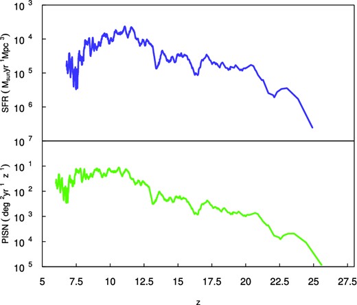
Top: The comoving formation rate density of Pop III stars as a function of redshift. Bottom: The intrinsic rate at which PISNe can be detected in the observer rest-frame (z = 0) as a function of redshift z.
3 SUPERNOVAE SPECTRAL ENERGY DISTRIBUTION SIMULATIONS
The PISN SED simulations account for the interaction of the blast with realistic circumstellar envelopes, the envelope opacity and Lyman α absorption by the neutral IGM at high redshift. We consider a set of models spanning the masses and metallicities of Pop III stars expected to die as PISNe (Joggerst & Whalen 2011; Whalen et al. 2013a). The mass range comprises 150, 175, 200, 225 and 250 M⊙ for zero-metallicity stars (z-series) and 10−4 Z⊙ stars (u-series) from the zero-age main sequence (table 1). All u-series stars die as red hypergiants and all z-series stars die as compact blue giants. Nevertheless, most 140–260 M⊙ Pop III stars have convective mixing and die as red stars instead of blue stars. The progenitor structure was evolved from the zero-age main sequence to the onset of collapse in the one-dimensional Lagrangian stellar evolution kepler code (Weaver, Zimmerman & Woosley 1978; Woosley, Heger & Weaver 2002) and the SN energy is determined by the amount of burned O and Si. The blast was followed until the end of all nuclear burning, when the shock was still deep inside the star. The energy generation is estimated with a 19-isotope network up to the point of oxygen depletion in the core and with a 128-isotope quasi-equilibrium network thereafter. The explosions were mapped in the Los Alamos Radiation Adaptive Grid Eulerian (rage) code Gittings et al. (2008) in order to propagate the blast through the interstellar medium. The extracted gas densities, velocities, temperatures and species mass fractions from rage are then interpolated on to a two-dimensional grid in the spectrum code (Frey et al. 2013), which calculates the SN SED.
In Fig. 2, we show an example of the PISN spectra evolution from breakout to 3 yr in the SN rest frame for model u175. The spectrum evolution over time is mainly dictated by two processes: (i) the fireball expands and cools, and its spectral cut-off advances to longer wavelengths over time; (ii) the wind envelope that was ionized by the breakout radiation pulse begins to recombine and absorb photons at the high-energy end of the spectrum, as evidenced by the flux that is blanketed by lines at the short-wavelength limit of the spectrum. At later times, flux at longer wavelengths slowly rises because of the expansion of the surface area of the photosphere. The SEDs are blue at earlier times and become redder as the expanding blast cools.
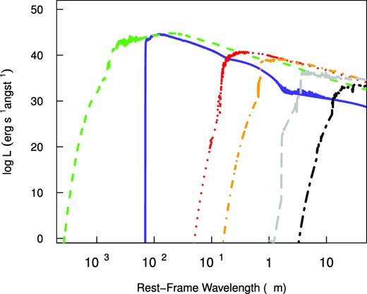
Rest-frame spectral evolution of the u175 PISNe. Fireball spectra at ≈1.291 d (green, short-dashed line), 1.306 d (blue, solid line), one month (red, dotted line), three months (orange, short-dashed-dotted line), 1 yr (grey, long-dashed line), 3 yr (black, long-dashed-dotted line).
Note that the SEDs used here have a peak bolometric luminosity that is an order of magnitude higher than those of Kasen et al. (2011). The following are a few effects that are included in our simulation, which might explain such a difference. (i) We include a wind profile around the stars that reach high temperatures when the shock crashes through the stellar surface. (ii) We implement two-temperature physics, thereby allowing radiation and matter to be out of thermal equilibrium, and thus more photons might be emitted by the flow. (iii) We use the Los Alamos National Laboratory OPLIB data base for atomic opacities instead of the Lawrence Livermore OPAL opacities1 (Iglesias & Rogers 1996; Rogers, Swenson & Iglesias 1996). We should also note that PISN luminosities are mainly driven by the conversion of kinetic energy into thermal energy by the shock at early times, and hence they are far brighter than Type Ia and II SNe at this stage. At later times, their higher luminosity comes from the larger amount of 56Ni compared with other SNe types (Whalen et al. 2013a).
4 INTERGALACTIC MEDIUM ABSORPTION
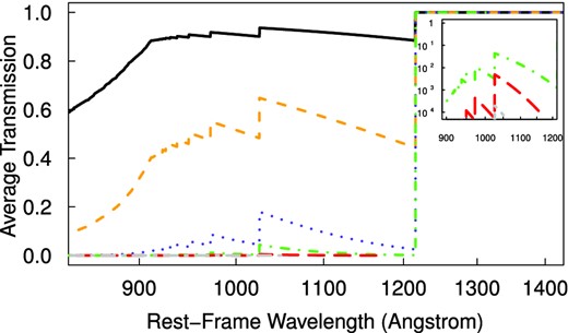
Attenuation of the UV continuum shortwards of Lyα due to neutral hydrogen along the line of sight. We show the average transmission of the IGM according to the Monte Carlo model of Meiksin (2006) for the following redshifts: z = 2 (black, solid line), z = 4 (orange, short-dashed line), z = 6 (blue, dotted), z = 7, (green, dotted-dashed line), z = 8 (red, long-dashed line) and z = 9 (grey, dotted-long-dashed line).
5 SURVEY IMPLEMENTATION
To simulate the observational process, we have implemented a modified version of the SuperNova ANAlysis (snana; Kessler et al. 2009) LC simulator. It consists of a complete package for SN LC analysis, including a LC simulator, a LC fitter and a cosmology fitter. snana provides an environment where we are able to design both sides of the observation process: the physical characteristics of the source-propagation medium and very specific observation conditions.
Any transient source can be included through a well-determined SED and explosion rate as a function of redshift. We include all models presented in Table 1, with a probability of occurrence given by the IMF described in Section 2.2. Other physical elements, such as the host galaxy extinction, IGM filtering and the primary reference star (which defines the magnitude system to be used), are convolved with the specific filter transmissions through the construction of k-correction tables. Such tables perform the translation from source-frame to observer-frame fluxes, on top of which the Milky Way extinction is applied by using full-sky dust maps (Schlegel, Finkbeiner & Davis 1998). We also include other telescope specifications, such as CCD characteristics, FOV, point spread function (PSF) and pixel scale.3
Parameters of PISN explosion models (Whalen et al. 2013a): pre-SN radius (R), helium core mass (MHe), mass of 56Ni synthesized in the explosion (MNi) and SN kinetic energy (E). The u-prefix models refer to the 10−4 Z⊙ metallicity progenitor, and the z-prefix models to zero metallicity, while the model number indicates the mass of the progenitor M⊙.
| Model | R (1013 cm) | E (1051 erg) | |$M_{\rm H_e}\, (\mathrm{M}_{\odot })$| | MNi (M⊙) |
|---|---|---|---|---|
| u150 | 16.2 | 9.0 | 72 | 0.07 |
| u175 | 17.4 | 21.3 | 84.4 | 0.70 |
| u200 | 18.4 | 33 | 96.7 | 5.09 |
| u225 | 33.3 | 46.7 | 103.5 | 16.5 |
| u250 | 22.5 | 69.2 | 124 | 37.9 |
| z175 | 0.62 | 14.6 | 84.3 | 0 |
| z200 | 0.66 | 27.8 | 96.9 | 1.9 |
| z225 | 0.98 | 42.5 | 110.1 | 8.73 |
| z250 | 1.31 | 63.2 | 123.5 | 23.1 |
James Web Space Telescope
The JWST will be an IR-optimized space telescope composed of four scientific instruments: a NIRCam, a near-infrared spectrograph (NIRSpec), a near-infrared tunable filter imager (TFI) and a mid-infrared instrument (MIRI) with enough fuel for a 10-yr mission (Gardner et al. 2006). Our analysis is based on NIRCam photometry in the 0.6–5 μm bands. One of the main targets of NIRCam is the exploration of the end of the dark ages. This is done by executing deep surveys of the sky covering a wide range of wavelength in order to optimize the estimate of photometric redshifts (Fig. 4). The JWST is expected to cover 30 per cent of the sky continuously for at least 197 continuous days. All points in the sky are expected to be surveyed over at least 51 d per year. The JWST will be able to observe any point within its field of regard (FOR; the fraction of the celestial sphere that the telescope can point towards at any given time) with a probability of acquiring a guide star of at least 95 per cent under nominal conditions (Gardner et al. 2006).
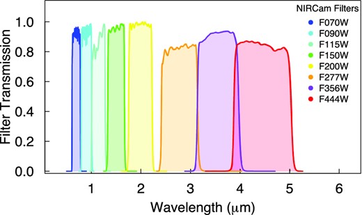
The set of JWST NIRCam filters implemented in our simulations.
To account for instrument characteristics, we use specifications from the NIRCam expected to be onboard the JWST (Fig. 4) and other technical features displayed in Table 2. All simulations presented here considered individual integrations of 102 s, which might sometimes be co-added to form a longer total exposure time. Note that ∼103 s is the limit for individual exposures due to cosmic ray contamination in the line of sight (Gardner et al. 2006). For the sake of completeness, we also show the explicit values for the zero-point, sky magnitude and error in sky magnitudes for each filter in Table 3. The CCD readout noise and sky-noise are determined by the CDD-NOISE and SKYSIG parameters (per pixel) summed in quadrature over an effective aperture (A) based on the PSF fitting, which we consider to be Gaussian.
The JWST technical specifications used to construct the simulation library: ZPTSIG, additional smearing to zero ZPTAVG; full width at half-maximum (FWHM); NIRCam FOV; mirror collecting area (A); pixel scale; CCD gain/noise (Gardner et al. 2006, and references therein).
| Feature | Value |
|---|---|
| CCD gain (e− ADU−1) | 3.5 |
| CCD noise (e− pixel−1) | 4.41 |
| Pixel scale (arcsec pixel−1) | 0.032 for F070W–F200W |
| 0.065 for F277W–F444W | |
| FWHM (pixel) | 2 |
| ZPTSIG (mag) | 0.02 |
| FOV (arcmin2) | 9.68 |
| A (cm2) | 2.5 × 10⁵ |
| Feature | Value |
|---|---|
| CCD gain (e− ADU−1) | 3.5 |
| CCD noise (e− pixel−1) | 4.41 |
| Pixel scale (arcsec pixel−1) | 0.032 for F070W–F200W |
| 0.065 for F277W–F444W | |
| FWHM (pixel) | 2 |
| ZPTSIG (mag) | 0.02 |
| FOV (arcmin2) | 9.68 |
| A (cm2) | 2.5 × 10⁵ |
Inputs used in the construction of the snana simulation library (SIMLIB) file for the JWST. Columns correspond to the NIRCam filter, zero-point for AB magnitudes (ZPTAVG), sky brightness (SKY) and error in sky brightness (SKYSIG). All values were calculated considering an exposure time of 103 s.
| NIRCam | ZPTAVG | SKY | SKYSIG |
|---|---|---|---|
| filter | (mag arcsec−2) | (mag arcsec−2) | (ADU pixel−1) |
| F070W | 27.87 | 27.08 | 1.24 |
| F090W | 28.41 | 26.90 | 1.34 |
| F115W | 28.89 | 26.76 | 1.39 |
| F150W | 29.51 | 26.88 | 1.35 |
| F200W | 30.20 | 26.96 | 1.34 |
| F277W | 30.85 | 26.32 | 1.75 |
| F356W | 31.38 | 26.75 | 1.43 |
| F444W | 31.88 | 25.58 | 2.47 |
After including JWST/NIRCam specifications, we are now left with the crucial task of building a proper observation strategy, one that maximizes our chances of measuring good quality LCs.
6 OBSERVATION STRATEGY
SN searches usually require multiple visits to the same area of the sky. The intervals between visits are determined by the typical redshift of the SN we are targeting, and the expected duration of its LC. The total area of the sky to be covered, or how many different fields will be monitored by our search, has to be chosen in agreement with the telescope scanning law. Because we expect to observe PISNe at high redshift (z ≥ 6), these objects will remain in the sky for a long time compared with the low-redshift SN counterpart. Despite their faintness, the redshift stretch allows us to draw the LC, making only a few observations per year of the same field.
The two observational strategies presented here are fully contained within the JWST flight plan (Table 4). We have also taken into account the fact that JWST will be able to make simultaneous observations with two filters (one at lower wavelengths and another at higher wavelengths).
Series of observational search strategies and selection cuts.
| Run | Sky (per cent) | Cadency | NIRCam filters | JWST time per yr |
|---|---|---|---|---|
| Strategy 1 | 0.06 | One pointing per year | F115W–F444W | 730 h |
| Strategy 2 | 0.06 | Three pointings per year, two-month gap | F150W, F444W | 730 h |
| Selection cuts | ||||
| At least one epoch before and one epoch after maximum | ||||
| Detection | ||||
| At least three epochs in one filter | ||||
| Cut 1 | At least one filter with S/N > 2 | |||
Strategy 1 consists of one pointing per year for each of the six reddest filters in NIRCam (F115W–F444W). This aims at maximizing our ability to identify these sources as high-redshift objects using non-detection in the bluest filters. Strategy 2 involves three pointings per year separated by two-month gaps for filters F150W and F444W. Its main goal is to define a LC shape for each event, allowing us to better distinguish it from other SN types. In both strategies, we use a 102 s exposure time for each pointing, during the total 5-yr telescope mission, corresponding to ∼730 h per year of telescope time and a total sky coverage of 0.06 per cent. As a matter of comparison, the Cosmic Evolution Survey (COSMOS) obtained a total of ∼1030 h of Hubble Space Telescope time4 (Koekemoer et al. 2007). Combining the information from different filters, we are able to roughly estimate the redshift of the source, because high-redshift objects disappear from the bluest filters. The detection of a PISN in all filters indicates a source at moderate redshift, z ≈ 6, while a detection only in the three reddest filters suggests z ≥ 15 (Fig. 5). Photometrically, the detection of a PISN among plenty of SN types, without redshift information, represents a challenge in itself (Fig. 6). Given the complexity of photometric classification methods (e.g. Ishida & de Souza 2013), we postpone this for future work.
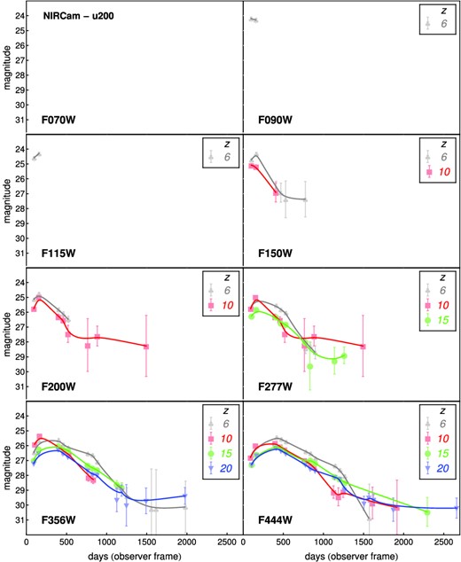
Examples of LCs from model u200 (Table 1), observed with NIRCam in eight different filters. We show the same LC as it would be observed by JWST for z = 6 (grey clubs), 10 (red squares), 15 (green circles) and 20 (blue inverted triangles). The observed magnitude is noted in the y-axis, while the x-axis represents the time in the observer frame. Observational strategies were built so that the LC evolution with redshift was optimized. The high-redshift events vanish from the bluest filters and their LCs last longer because of time dilation.
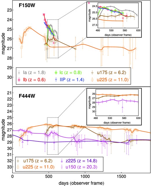
LCs from PISN models (Table 1) superimposed with core collapse and Type Ia LCs. Top: u175 (z = 6.2, brown diamonds), u225 (z = 11.0, orange open squares), Type Ia (z = 1.8, grey clubs), Type Ib (z = 0.6, red squares), Type Ic (z = 0.8, green circles) and Type IIP (z = 1.4, blue inverted triangles) observed through filter F150W. Bottom: u175 (z = 6.2, brown diamonds), u225 (z = 11.0, orange open squares), z225 (z = 14.8, purple triangles) and u150 (z = 20.3, pink open circles) observed through filter F444W. The observed magnitude is noted in the y-axis, while the x-axis represents the time from the first detection in the observer frame. Observational strategies were chosen so that individual features of different SN types were emphasized. With standard SN searches running for a few months (zoomed in region), it is difficult to distinguish PISN LCs from other SN types (top) or among themselves (bottom). Longer observing plans using multiple filters are better suited to photometrically classifying these events.
Assembling all ingredients described so far, we were able to generate a catalogue of PISN LCs. The final step is to define a minimum requirement for a SN to be ‘detected. Based on our goal of identifying these objects as transients, it is crucial to obtain at least a few observations near the LC peak. Therefore, for an object to be considered detected, we demanded at least one epoch before and one epoch after maximum brightness. We also required the detection of three epochs in at least one filter above the background limit. Here, we present results for a signal-to-noise ratio (S/N) selection cut of S/N ≥ 2 in at least one filter (Fig. 7). More restrictive cuts might become infeasible in terms of the JWST allocation time. Nevertheless, we should point out that the framework described so far is flexible enough to accommodate any observational strategy, SFR, SN SED, and other missions as well.
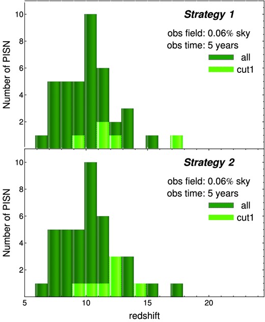
Number of PISNe as a function of redshift for one survey realization. Dark-green histograms correspond to all SN events in the observed field (SNe/Field). Light-green histograms represent PISNe with at least one filter having S/N > 2 (cut 1). The upper panel shows results from strategy 1, (40 SNe per field, five SNe satisfying cut 1) and the lower panel displays outcomes from strategy 2 (40 SNe per field, seven SNe satisfying cut 1).
Using the complete framework, we obtained 5 ± 3 PISN detections from strategy 1 and 7 ± 4 PISN from strategy 2 (averaged over 100 realizations), both satisfying S/N ≥ 2 (Fig. 5). This is a clear indication that the JWST will be able to observe a handful of PISNe, but not without using a significant amount of telescope time. In the two strategies, a minimum of one month per year of allocation time is necessary to obtain ∼1–2 detections per year. It should be noted that these predictions are obtained under very conservative assumptions. Accounting for uncertainties in Pop III SFR and IMF could increase our results up to 43 ± 10 and 75 ± 15 detections (or even more) for strategies 1 and 2, respectively (see Fig. A1).
We show that, given a fixed amount of telescope time, changing the observation strategy might increase the number of detections. This suggests that strategy 2, consisting of three pointings per year with only two filters, results in more detections than strategy 1. Once potential candidates are detected, the brightest sources will be suitable for more detailed follow-ups, thereby placing strong limits on their metal content. For low-metallicity objects, the ratios of oxygen lines to Balmer lines, such as [O iii]/Hβ, provides a linear measurement of metallicity.
A complementary search might be possible with upcoming NIR surveys, such as WFIRST,5 the Wide-field Imaging Surveyor for High-redshift6 (WISH) and Euclid.7 A multiwavelength approach is also possible by using Pop III SN signatures in the 21-cm signal with future radio facilities such as the Expanded Very Large Array8 (EVLA), e-MERLIN9 and the Square Kilometre Array10 (SKA; Meiksin & Whalen 2013). Primordial SNe observed by deep surveys might act as evidence of primordial galaxies, and plenty of primordial objects might be unveiled, such as GRB orphan afterglows, a comprehensive zoo of high-redshift SN types, core-collapse (Whalen et al. 2013b) and Type IIn (Whalen et al. 2013c), or even unexpected novel transients pervading the infant Universe.
7 CONCLUSIONS
We simulate the detectability of PISNe in the most realistic way to date, thereby constructing the first synthetic survey of high-redshift SNe. We make use of advanced cosmological and radiation hydrodynamics simulations combined with detailed modelling of the observational process and IGM absorption. Under very conservative assumptions, we show that observing Pop III stars, through their deaths as PISNs, is feasible with JWST-type missions, but not without a commitment in terms of telescope allocation time. In agreement with Hummel et al. (2012), we find that the scarcity of the events and, consequently, the sky coverage are limiting factors in detecting PISNe, rather than their faintness. We show that a dedicated observational strategy using ≲ 8 per cent of total allocation time of the JWST mission can provide us with up to ∼9–15 detectable PISNe per year, accounting for possible uncertainties in Pop III IMF and stellar evolution models.
Additionally, we show that the combination of multiple filter information is crucial to detect and distinguish high-redshift SN candidates from their low-redshift counterparts. We have not discussed the minimum requirements (S/N, number of detections, number of filters, etc.) needed to photometrically classify these objects for posterior spectroscopic confirmation. Because of time dilation, the SN LCs remain in the sky for a couple of years, requiring an extended survey to detect these objects as transients. The most promising way should be to find these events with an IR mission with a larger FOV, such as Euclid, and after identifying the interesting candidates, to perform a more careful analysis with the JWST. Given the level of detail in simulating the observing process, our synthetic sample might be easily used to calibrate photometric classification techniques. We leave this discussion, together with the inclusion of other SN SEDs, such as core-collapse and Type IIn, and the Euclid specifications for subsequent work. Because of its comprehensive nature, our synthetic survey of PISNe represents a leap forward in high-redshift SN studies. It demonstrates what we expect to be unveiled about the early Universe during the next decade.
We thank Andrea Ferrara and Naoki Yoshida for their careful revision of this manuscript. We thank Rick Kessler for valuable help in dealing with snana. We also thank G. Lima Neto for constructive suggestions and L. Sodré Jr, for the encouragement in the early stages of this project. Finally, we thank A. Jendreieck, A. Sodero, C. Boyadjian, F. Fleming and M. Pereira for useful comments. DJW acknowledges support from the Baden-Württemberg-Stiftung by contract research via the programme Internationale Spitzenforschung II (grant P- LS-SPII/18). EEOI thanks the Brazilian agency FAPESP (2011/09525-3) for financial support. RSS and EEOI thank the Max Planck Institute for Astrophysics for hospitality during the development of this work.
For all simulations presented here, we use AB magnitudes.
REFERENCES
APPENDIX A: DEPENDENCE WITH SUPERNOVA RATE
The PISN rate is subject to a number of uncertainties, some of which are described here.
Initial mass function
We have adopted an IMF with lower and upper limits of 21 and 500 M⊙. If we instead consider a top-heavy IMF with a range of mass within 100–500 M⊙, the efficiency in creating PISNe (given by the integral over IMF in the range 140–260 M⊙) would increase by a factor of ∼10.
Stellar evolution models
The predicted initial mass range of 140–260 M⊙ for PISN progenitors is for non-rotating stars (Heger & Woosley 2002). However, the first stars could have fast rotation (Stacy, Bromm & Loeb 2011). Chatzopoulos & Wheeler (2012) have found that rotating stars with masses >65–75 M⊙ can produce direct PISN explosions as a result of a more chemically homogeneous evolution, which leads to increased oxygen core masses. Assuming our fiducial IMF, this would increase the PISN fraction by a factor of ∼4.
Simulation box size
At high redshift, galactic haloes are rare and correspond to high peaks in the Gaussian probability distribution of initial fluctuations (Barkana & Loeb 2004). In numerical simulations, periodic boundary conditions are usually assumed, thereby forcing the mean density of the box to equal the cosmic mean density. This sets density modes with wavelengths longer than the box size (4 Mpc in our case) to zero, resulting in an underestimate of the mean number of rare, biased haloes. Accounting for these missing modes (Barkana & Loeb 2004), we estimate that the true SFR at z = 7 (20) could be larger by a factor of ∼1.3 (7) if star formation is dominated by atomically cooled haloes, or by a factor of ∼1.1 (2) if star formation is dominated by molecularly cooled haloes.
To account for the above uncertainties in our final results, we rerun the simulation with a 10 times higher Pop III PISN rate as a more optimistic case (Fig. A1). This value is in agreement with observational constraints from cosmic metallicity evolution and the local metallicity function of the Galactic halo (Rollinde et al. 2009). It sets an upper limit of 3 × 10⁻³ M⊙ yr−1 Mpc−3 for Pop III SFR at any redshift. Furthermore, recent observations from high-redshift long GRBs suggest that the SFR could be around ∼10−3–10−2 M⊙ yr−1 Mpc−3 at z = 10 (Ishida, de Souza & Ferrara 2011; Robertson & Ellis 2012). Hence, a combination of the Pop III SFR upper limit imposed by observations and uncertainties in the IMF could allow a PISN rate 100 times higher than our fiducial model as an extreme case.
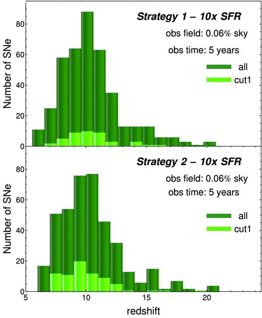
Number of PISNe as a function of redshift for one survey realization considering a 10× higher PISN rate at all redshifts. Dark-green histograms correspond to all SN events in the observed field (SNe per field). Light-green histograms represent PISNe with at least one filter having S/N > 2 (cut 1). The upper panel shows results from strategy 1 (404 SNe per field, 46 SNe satisfying cut 1) and the lower panel displays outcomes from strategy 2 (404 SNe per field, 73 SNe satisfying cut 1).
