


Abstract
We examine and combine different techniques that are known to increase the Fisher information content about the amplitude of the matter power spectrum, and propagate their impact on a baryonic acoustic oscillation (BAO) measurement. We compare a density reconstruction algorithm based on Zel'dovich displacement fields, a wavelet non-linear Wiener filter, a direct Gaussianization of the probability distribution function of the wavelet function coefficients and the action of the last two techniques on the first one. From a series of 200 N-body simulations, we compute the Fisher information and quantify the recovery performance, both using dark matter particles and haloes. We find that the height of the Fisher information trans-linear plateau is generally increased by the various techniques, by up to an order of magnitude at k = 0.6 h Mpc−1; however, shot noise subtracted halo measurements exhibit a milder information recovery. When we perform a BAO measurement from these altered density fields, we find that the reconstruction technique is the only one that sharpens the peak; the two wavelet-based techniques in fact smear out the features, thus reducing the overall precision of the cosmological ladder. We examine in detail why this occurs even though their Fisher information increased.
INTRODUCTION
Understanding the nature of dark energy has been identified internationally as one of the main goals of modern cosmology (Albrecht et al. 2006), and many dedicated experiments attempt to constrain its equation of state: LSST1 (LSST Science Collaboration 2009), Euclid2 (Beaulieu et al. 2010), JDEM3 (Gehrels 2010), CHIME4 (Peterson, Bandura & Pen 2006), SKA5 (Schilizzi 2007; Dewdney et al. 2009), BOSS6 (Schlegel, White & Eisenstein 2009) and Pan-STARRS.7 One of the favoured techniques involves a detection of the baryonic acoustic oscillation (BAO) signal (Seo & Eisenstein 2003, 2005; Eisenstein, Seo & White 2007; Seo & Eisenstein 2007), which has successfully constrained the dark energy parameter in current galaxy surveys (Eisenstein et al. 2005; Tegmark et al. 2006; Percival et al. 2007; Blake et al. 2011). The analyses are based on a detection of the BAO wiggles in the matter power spectrum, which act as a standard ruler and allow one to map the cosmic expansion.
With the new and upcoming generation of dark energy experiments, the precision at which we will be able to measure the cosmological parameters is expected to drop at the sub-per cent level; therefore, it is essential to understand and suppress every sources of systematic uncertainty. In a BAO analysis, one of the main challenges is to extract an optimal and unbiased power spectrum from the data, along with its uncertainty; the latter propagates directly on the dark energy parameters with Fisher matrices (Fisher 1935; Tegmark, Taylor & Heavens 1997) or likelihood analyses. This task is difficult for a number of reasons. For instance, the scales that are relevant for the analyses sit at the transition between the linear and the non-linear regimes, at least for the redshift at which current galaxy surveys are sensitive; hence, the underlying uncertainty on the matter power spectrum is affected by the non-linear dynamics. These effectively couple the phases of different Fourier modes (Zhang et al. 2003) such that the Gaussian description of the density fields has been observed to fail (Meiksin & White 1999; Rimes & Hamilton 2005, 2006; Neyrinck, Szapudi & Rimes 2006; Neyrinck & Szapudi 2007). For an estimate of the BAO dilation scale to be robust, one must therefore include in the analysis the full non-linear covariance of the power spectrum. Although results from Takahashi et al. (2011) seem to suggest that non-Gaussianities had no real effect on the final results, it was recently shown that this was only true if the original power spectrum was measured in an unbiased and optimal way, which is rarely the case (Ngan et al. 2012). Otherwise, the discrepancy on the constraining power is at the per cent level.
One way of reducing the impact of the non-linear dynamics is to transform the observed field into something that is more linear. Over the last few years, many ‘Gaussianization’ techniques (Weinberg 1992) have been developed, which all attempt to undo the phase coupling between Fourier modes. The number of degrees of freedom – i.e. uncoupled phases – can be simply quantified by the Fisher information about the power spectrum amplitude, and recovering parts of this erased information can lead to improvements by factors of a few on cosmological parameters.
For example, a density reconstruction algorithm (Eisenstein et al. 2007b; Noh, White & Padmanabhan 2009; Padmanabhan, White & Cohn 2009) has been shown to reduce the constraints on the BAO dilation scale by a factor of 2 (Eisenstein et al. 2007b; Ngan et al. 2012). Based on the Zel'dovich approximation, it effectively displaces the simulated (or observed) objects to an earlier time, in a state where the density field is more Gaussian, i.e. where departures from Gaussianity are weaker and occur at smaller scales. This technique was recently applied on the Sloan Digital Sky Survey data (Padmanabhan et al. 2012) to improve the BAO detection, with small modifications to the algorithm so as to correct for the survey selection function and redshift space distortions. As discussed therein, an important issue is that two main mechanisms are reducing our ability to measure the BAO ring accurately: (1) a large coherent ∼50 Mpc infall of the galaxies on to overdensities, which tends to widen the BAO peak, and (2) local non-linear effects, including non-linear noise, which also erase the smallest BAO wiggles. Reconstruction addresses the first of these mechanisms, and it is important to know whether something can be done about the second, after reconstruction has been applied.
Wavelet non-linear Wiener filters (hereafter WNLWF, or just wavelet filter) were used to decompose dark matter density fields (Zhang et al. 2011) and weak gravitational lensing κ-fields (Yu et al. 2012) into Gaussian and non-Gaussian parts, so as to condense in the latter most of the collapsed structure; the Gaussian part was then shown to contain several times more Fisher information than the original field. This technique seems well suited to address the issue of non-Gaussian noise described above, but is not the only promising approach. A direct Gaussianization of the wavelet function coefficients (hereafter DGWFC) can potentially do the same trick, and other methods, including Cox–Box transformations (Joachimi, Taylor & Kiessling 2011), running N-body simulation backwards (Goldberg & Spergel 2000) or direct Gaussianization of the one-point probability function (Yu et al. 2011), could be investigated as well for a thorough study.
Our focus, in this paper, is to discuss how some of these techniques can be used in conjunction to maximize the recovery of Fisher information about the amplitude of the matter power spectrum. The cosmological application is immediate, as a higher information content in the range k ∼ 0.2–1.0 h Mpc−1 means smaller error bars on the BAO signal, and hence tighter constraints on dark energy. Not all combinations of Gaussianization techniques are good match, however. It was recently shown (Yu et al. 2012) that WNLWF and log-normal transforms (Neyrinck, Szapudi & Szalay 2009; Seo et al. 2011) are not interacting in an advantageous way. On one hand, if the log-normal transform is applied on to a Gaussianized field, the prior on the density field is no longer valid, and the log-normal transform maps the density into something even less Gaussian. On the other hand, it was shown that the log-normal transform is less effective than WNLWF alone at recovering Fisher information, at least on small scales. Applying the filter after the log-normal transform does not improve the situation, since the Gaussian/non-Gaussian decomposition is less effective. In other words, the Fisher information that the log-normal transform could not extract is not recovered by WNLWF, and we are better off with the WNLWF alone.
It seems, however, that this unfortunate interaction is not a constant across all combinations. In this paper, we discuss how either direct Gaussianization or non-linear Wiener filters (NLWF) constructed in wavelet space can improve the results of the density reconstruction algorithm. We first obtain these results with particle catalogues extracted from N-body simulations, and extend our techniques to halo catalogues, which provide a sampling of the underlying matter field that is much closer to actual observations. We find that in both cases, these techniques (reconstruction + WNLWF and reconstruction + DGWFC) work well together, in the sense that the final Fisher information recovery is larger than the two stand-alone techniques.
It is tempting at this point to declare that we have found an optimal Fisher information recovery pipeline; however, further investigations prove that this conclusion could not be reached that simply. When looking at the cross-correlation between the initial and final fields – i.e. the propagator – for these different techniques, it turns out that both wavelet techniques lose information about the primordial field, well in the BAO regime. Although this loss is not quite large, it is then legitimate to ask: what it means, then, to have a higher Fisher information? In that context, then, what is this information about? Are we gaining anything in the end? To answer these questions, we are left with no choice but to propagate the error on to a typical analysis pipeline and compute constraints on the BAO scale. Our results show that in fact, the gain in Fisher information does not always compensate for the loss about the primordial BAO wiggles; hence, one should be careful about hasty conclusions drawn solely from Fisher information recovery.
The structure of the paper is as follows: in Section 2, we describe our N-body simulations, we briefly review the theoretical background of the density reconstruction, the WNLWF and the DGWFC, and detail how we extract the density power spectra, their covariance matrices and the Fisher information; we present our results in Section 3. The propagator calculations and the Fisher forecast for the BAO analysis are presented in Section 4, and we finally discuss the implications of our findings in Section 5.
THEORETICAL BACKGROUND
Numerical simulations
Our sample of 200 simulations are generated with cubep3m (Harnois-Déraps et al. 2012), a high-performance N-body code that solves the Poisson equation on a two-level mesh with sub-grid resolution, thanks to the p3m calculation. Each run evolves 5123 particles on a 10243 grid, and is computed on a single IBM node of the Tightly Coupled System (TCS) on SciNet (Loken et al. 2010) with ΩM = 0.279, ΩΛ = 0.721, σ8 = 0.815, ns = 0.96 and h = 0.701. We assume a flat universe and find the initial position and velocity of the particles at zi = 50 with the Zel'dovich approximation. Each simulation has a side of 322.36 h−1Mpc, and we output the particle catalogue at z = 0.054.
We search for haloes with a spherical overdensity algorithm (SO; Cole & Lacey 1996) executed at run time, which sorts the local grid density maxima in descending order of peak height, then loops over the cells surrounding the peak centre and accumulates the mass until the integrated density drops under the collapse threshold of Δ = 178, and finally empties the contributing grid cells before continuing with the next candidate, ensuring that each particle contributes to a single halo. Halo candidates must consist of at least one hundred particles, ensuring that the haloes are large and collapsed objects. The centre of mass of each halo is calculated and used as position, as opposed to its peak location, even though both quantities differ by a small amount. We mention here that algorithms of this kind have the unfortunate consequence of creating an exclusion region around each halo candidate, with no sub-haloes, thus effectively reducing the resolution at which the halo distributions are reliable. Each field contains about 88 000 haloes, for a density of 2.6 × 10⁻³ h3 Mpc−3. For comparison, this is about eight times larger than the BOSS density (Schlegel et al. 2009).
Density reconstruction algorithm
In our numerical calculations, the particles and haloes are assigned on to the grid with a cloud-in-cell (CIC) interpolation scheme (Hockney & Eastwood 1988), and the displacement fields are actually obtained by finite differentiation of the (late-time) potential field.
Wavelet non-linear Wiener filter (WNLWF)
In this sub-section, we briefly review the WNLWF algorithm, and direct the reader to Zhang et al. (2011) and Yu et al. (2012) for more details.
We consider in this paper the Daubechies-4 (Daubechies 1992) discrete wavelet transform, which contains certain families of scaling functions ϕ and difference functions (or wavelet functions) ψ. The density fields are expanded into combinations of these orthogonal bases, and weighted by scaling function coefficients (SFCs) and wavelet function coefficients (WFCs). In our WNLWF algorithm, we deal only with the latter, each of which characterizes the amplitude of the perturbation on a certain wavelength and at a certain locations.
In the three-dimensional case, the properties of each perturbation depend on three scale indices (j1, j2, j3) – controlling the stretching of the wavelet Daubechies-4 functions – and three location indices (l1, l2, l3) – controlling their translation. Specifically, in a given dimension, the grid scale corresponding to a specified dilation is L/2j (2j = 1024 in our case), and the spatial location is determined by lL/2j < x < (l + 1)L/2j. After the wavelet transform, all SFCs and WFCs are stored in a three-dimensional field, preserving the grid resolution (see Fang & Thews 1998; Press et al. 1992 for more details).
The NLWF acts on individual wavelet modes, which are defined as combinations (not permutations) of all WFCs having the same three scale indices (j1, j2, j3). For each wavelet mode, the NLWF is determined completely by the PDF of the corresponding WFCs, fPDF(x), which is constructed by looping over the other three indices (l1, l2, l3).8
We emphasize on the fact that the filter functions depend only on the parameter s, which is the full width at half-maximum of the Gaussian NLWF window function wG. It characterizes the extent of the departure from a Gaussian PDF: the greater the s, the smaller the departure from Gaussian statistics. The same decomposition is performed on the reconstructed density fields and on those obtained from the halo catalogues. In this paper, we do not make use of the information contained in the non-Gaussian component and simply discard it, although it serves as a powerful probe of small-scale structures and could help identifying haloes in a (Gaussian) noisy environment.
Direct Gaussianization of wavelet function coefficients (DGWFC)
The last Gaussianization technique used in this paper is inspired by the method of Weinberg (1992), with the modification that we apply the technique on the PDF of the WFCs, as opposed to that of the real space distribution. As discussed in the previous section, the PDF of the WFC clearly reflects the non-Gaussian properties of the underlying field; hence, a DGWFC has the potential to do exactly what we need, that is, to smooth out (or undo some of) the non-Gaussian features of the density fields.
Information recovery
The calculation of uncertainty about dark energy cosmological parameters is based on the propagation of the uncertainty about the matter power spectrum. In this process, the number of degrees of freedom – i.e. the Fisher information – contained in the field is directly related to the constraining power. In this section, we briefly review how we calculate the Fisher information content in the amplitude of the matter and halo power spectra.
In the current paper, we used 200 simulations to extract the power spectrum covariance matrix about 16 k-bins; therefore, the estimate of inverse covariance would be about 10 per cent biased on the high side, at least in the linear regime. However, the unbiased estimator proposed by Hartlap et al. (2007) is only valid in Gaussian statistics, whereas our measurements are sitting at the transition between the linear and the non-linear regimes; hence, it is not clear how the proposed correction would actually improve the estimate. In any case, this inversion bias is constant for all the measurements we made, and since we are ultimately interested about the ratio between them, the correction factor would cancel out. For these reasons, we do not include this correction factor in the figures.
RESULTS
In this section, we describe and quantify our ability at recovering the Fisher information content in the amplitude of the matter power spectrum, with our three Gaussianization techniques, for density fields measured with either simulated particles or haloes. We first present visually the effect of the techniques, and then present the power spectrum, covariance and Fisher information measurements.
Density fields
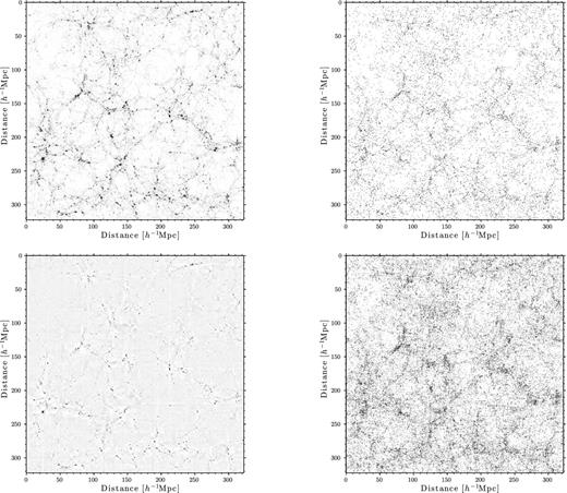
To illustrate the effect of different Gaussianization techniques, we present in Fig. 1 the projections through a thickness of 200 cells of a given realization after density reconstruction alone, after WNLWF or DGWFC alone, and with one of the two wavelet techniques applied on the reconstructed density. We observe that the reconstruction reduces the size of each halo, and blurs out the smaller ones, as expected from this algorithm: particles generally tend to travel outwards from the gravitational well. WNLWF has a different effect on the density: it removes most of the smallest structure perturbations, leaving behind only the larger modes. Visually, it looks like some kind of smoothing was applied on the field. As discussed in Pen (1999), the geometry of the Cartesian wavelet sometimes leaves behind grid patterns, which only affects the smallest scales of the power spectrum – in this case k > 8.0 h Mpc−1. It would be feasible, in principle at least, to attempt a compression or a removal of these artificial structures, but we left that aside since it has no impact on the scales we are interested in. The combination of both techniques is presented in the middle-right panel, which visually presents the least amount of collapsed structures, although the largest clusters remain. The DGWFC is also presented in the bottom panels, where we also see a suppression of the smallest haloes.
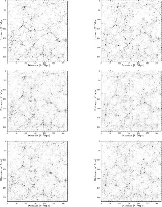
Projections through a thickness of 200 cells of one of the realizations. In each panel, the side is 322.36 h−1 Mpc, and the image contains 10242 pixels. Top left shows the original field, top right shows the field after density reconstruction, middle panels show the WNLWF field (Gaussian part) with (right) and without (left) density reconstruction, and the bottom panels show the DGWFC field with (right) and without (left) density reconstruction. To ease the visual comparison, each panel shows the same overdensity range and saturates for denser regions, i.e. all pixels with δ > 5 are black. The non-Gaussian part of the wavelet filtered fields is discussed in Appendix A, along with results for the haloes.
For completeness, we discuss in Appendix A the non-Gaussian part of the two wavelet techniques and compare with the halo distributions. We see how one traces the other, which illustrates the power of the technique.
Power spectrum and covariance
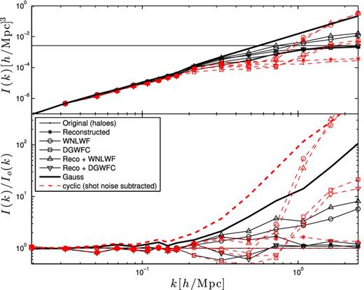
Fig. 2 shows the power spectrum of the dark matter particles and haloes before and after the Gaussianization techniques. In order to achieve convergence on the covariance matrices at a later stage of the analysis, while preserving most of the information in the BAO regime, it is necessary to choose carefully the binning of the power spectrum. It was shown in Ngan et al. (2012) that the Fisher information about the power spectrum amplitude was insensitive to binning, and we have 200 simulations at our disposal. Since convergence on the matrix is achieved when the number of simulation approaches the number of elements to be measured, and that we need to span the two decades in k that are resolved, it is not possible to keep a linear binning all the way. Instead, we bin our measurements in linear space up to k = 0.15 h Mpc−1, and then switch to log space.
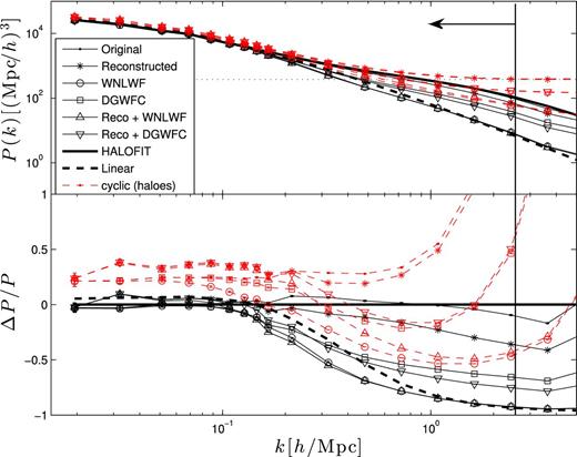
Top: power spectra of the original and Gaussianized fields, from simulated particles (symbols + solid lines) and haloes (symbols + dashed line). The linear and non-linear predictions from halofit are shown by the thick dashed and solid lines, respectively, and the Poisson noise corresponding to the halo population is shown with the thin horizontal dotted line. Bottom: fractional error between the curves of the top panel and the non-linear prediction from halofit. We observe that the particle power spectrum deviates by more than 10 per cent for k > 2.5 h Mpc−1, which sets the resolution limit of our simulations. This scale is represented by the vertical line in both panels. The original and reconstructed halo power spectra are shot noise dominated at scales smaller than k ∼ 1.0 h Mpc−1.
We first observe that the measurement from the original particle field agrees to within 10 per cent level with the non-linear predictions obtained from halofit (Smith et al. 2003) up to k ∼ 2.5 h Mpc−1, which sets the resolution scale of our power spectrum measurements.10 That way, our measurements comprise 16 bins in total. The Gaussian component of the WNLWF preserves more than 95 per cent of the power on linear scales – up to k ∼ 0.1 h Mpc−1 – after which the signal from trans-linear and non-linear scales is mostly transferred to the non-Gaussian contribution, and hence the drop in power. We note that the wavelet filtered power spectrum traces the linear predictions to within a factor of 2 up and beyond k ∼ 4.0 h Mpc−1. This illustrates how shot noise, which typically contributes only at relatively small scales, can be filtered out by the WNLWF. The power spectrum of the DGWFC fields has similar trends, in that it closely follows the original fields up to k ∼ 0.1 h Mpc−1 and drops at smaller scales, although the resulting small-scale power is about 20 per cent higher than that of the WNLWF. This is caused by the fact that these small scales are not filtered out but rather Gaussianized, and hence still have an imprint in the final field. The density reconstruction algorithm also has a significant impact on the shape of the power spectrum on small scales, since particles are pumped out of the gravitational potential. As a result, power from k > 0.1 h Mpc−1 is reduced, as seen in the figure.
In the linear regime, the power spectra from the WNLWF and the DGWFC acting on the reconstructed fields (Reco + WNLWF and Reco + DGWFC in the figure) trace at the few per cent level the effect of the reconstructed algorithm alone, and then catch up with their respective stand-alone techniques by k ∼ 0.1 h Mpc−1. This observation suggests that the advantages of these two techniques might reinforce one another, as they preserve the effect of reconstruction in the largest scales, but suppress the non-linear structures. The question that needs to be addressed is whether this suppression impacts in a positive way the performance with which we can extract the BAO measurement. We come back to this in Section 4.
When looking at the halo measurements, we observe that the original and reconstructed power spectra are both dominated by shot noise at scales smaller than k ∼ 1.0 h Mpc−1, and that this noise is strongly suppressed by the two wavelet filter techniques for reasons explained above. The WNLWF power spectrum is also only a factor of 2 away from the linear predictions up to k ∼ 0.7 h Mpc−1. and the DGWFC is about 20 per cent higher. We measure a linear halo bias of b2 ∼ 1.2 from the original halo fields. As for particles, the three stand-alone techniques tend to suppress the small-scale power compared to the original fields, and in the case where the techniques are combined, this suppression is 5–10 per cent weaker. This is probably related to the fact that the linear bias seems to be increased by about 15 per cent by the reconstruction algorithm, since a rescaled version of this plot, where the linear scales all match, would show a stronger suppression in combined techniques.
Note that in Fig. 2, the shot noise has not been subtracted. In practice, a common way to deal with the Poisson noise is to compute the cross-power spectrum between two populations randomly selected out of the original catalogue. The shot noise is averaged out in this operation, and the signals left behind are stronger on large and intermediate scales. In our calculations, small scales are typically anticorrelated due to the ‘halo exclusion’ effect, which is a result of our halo finder: the algorithm effectively collapses all the structure of a given halo to a single point, and leaves empty the region surrounding the centre of mass, with no sub-halo. In that regime, then, the cross-power spectrum becomes negative, and should therefore be excluded from the analyses. Although precise and robust, this procedure is difficult to apply to all the cases under study in this paper. In particular, the density reconstruction algorithm requires an accurate measurement of the gravitational potential; the halo exclusion effect already undermines the extracted gravitational potential, and the accuracy of this technique would suffer heavily if we removed half of the haloes. To estimate the noise-free power spectrum, we use another common approach that consists in subtracting from the measurement a flat shot noise, defined as |$P_{\rm shot} = 1/n = L^{3}/N_{\rm {\rm haloes}}$|. This technique is much faster and completely compatible with the requirements of our algorithms; however, the resulting noise appears to be overestimated compared to the cross-power approach. This was noted before by Jing (2005), who recommended a more sophisticated approach that we delayed for future work. A better estimate of the noise in the halo distribution is therefore the product of Pshot and a scale-dependent bias, but in order to avoid any systematics associated with such an operation, we decided to preserve the original, conservative noise estimate.
To quantify how this simple noise filtering performs, we show in Fig. 3 a comparison between the original halo power spectrum from the full catalogue, the cross-spectrum and the ‘naive’ shot noise subtracted power. We observe that the two shot noise subtraction techniques agree up to k = 0.3 h Mpc−1, beyond which the P(k) − Pshot(k) approach filters out more power; by k = 1.0 h Mpc−1, the leftover signal is smaller by a factor of 2.4. For even smaller scales, the shot noise subtracted power starts to increase, a clear sign that our shot noise estimator completely fails beyond that point. The difference between the two shot noise subtraction techniques means that our simple approach is not optimal, as we are losing too much power on scales in the range [0.3-1.0] h Mpc− 1. The impact of this suppression on the covariance matrices should be mild, however, as these are insensitive to additive constants.
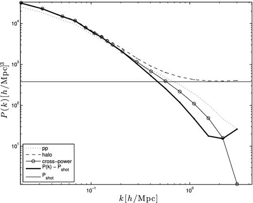
Comparison between different shot noise subtraction techniques for a single density field. The dashed line shows the halo power spectrum of the full population, the dotted line shows the power spectrum of the particles, the open symbols represent the cross-spectrum of two randomly selected sub-populations, the horizontal straight line shows the naive Poisson noise estimate and the thick solid line shows the shot noise subtracted estimate we adopt in this paper: P(k) − Pshot.
Covariance matrices
The three Gaussianization techniques that are discussed in this paper attempt to bring cosmological information, or degrees of freedom, back to the power spectrum. Consequently, the covariance matrices of the Gaussianized fields are expected to be more diagonal. The top-left panel of Fig. 4 shows the cross-correlation coefficient matrix of the original particle fields in the upper triangle, and the reconstructed ones on the lower triangle. To ease the comparison between the figures, we show in the panel the positive components only and the negative entries in the insets. Most of the off-diagonal elements of the covariance matrix are reduced to under 40 per cent correlation by the reconstruction algorithm. There is a mild anticorrelation (less than 30 per cent) in some matrix elements of the reconstructed fields, which comes from residual noise in the largest scale. This noisy effect has very little impact, except for the undesired featured that the information content is allowed to exceed that of the Gaussian case. To correct for it, we impose a prior that the underlying matrix has no negative elements, as established from performing similar analyses with thousands of simulations (Takahashi et al. 2009; Ngan et al. 2012). We therefore assume that the negative elements we are measuring are noisy, and set them to zero beyond this stage. This surely introduces a bias since it is a one-way levelling, i.e. no positive elements are lowered. As a result, the inverse of the matrix, which we are interested in, is probably a little bit on the low side. However, this only occurs at k ∼ 0.15 h Mpc−1, and the bias becomes negligible as high k-modes are included.
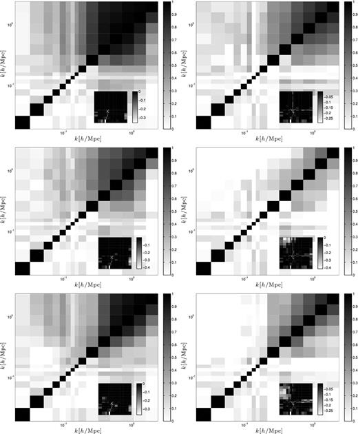
Top left: cross-correlation coefficient matrix associated with the particle power spectra. The top triangle represents measurements from the original matter fields, while the lower triangle elements are from fields after the reconstruction technique has been applied. The inset quantifies the amount of anticorrelation between the measurements, and has the same binning and axis scales as the main figure. Middle left: the top triangle represents measurements from the WNLWF, while the lower triangle represents measurements from fields that are first reconstructed, and then wavelet filtered – still using particles as tracers. Bottom left: the top triangle shows results from the DGWFC, while the lower triangle shows results from fields that are first reconstructed, and then directly Gaussianized. Right-hand panels: same as the left-hand panels, but for haloes.
Back to Fig. 4, the middle-left panel shows, on the upper triangle, the results after the WNLWF has been executed, and the combination with reconstruction in the lower triangle. The off-diagonal elements of the covariance matrix are also reduced by 20–40 per cent in both cases, although the combination is more diagonal than both techniques alone. The bottom-left panel shows DGWFC in the upper triangle, and the combination with reconstruction in the lower triangle. Although the DGWFC is less performant than the NLWF, we observe that the combination with the reconstruction diagonalizes very well the covariance matrix.
The right-hand panels of Fig. 4 show the equivalent measurements carried on halo fields, without the shot noise subtraction. The original fields show weaker correlations compared to particles to start with, which is caused by the fact that the non-linear dynamics are blurred by the Poisson noise, and by the halo exclusion effect, which prevents us from seeing details about regions that are gravitationally collapsed. We observe that the density reconstruction algorithm has a milder impact on the correlation of the halo measurements. As explained before, this is caused by the fact that the region of exclusion about each simulated halo prevents an accurate construction of the gravitational potential.11 This is a strong limit of the technique using our current halo finder, as real galaxies behave much more like haloes than particles, and many are satellites. Fortunately, data do allow for higher multiplicity in the galaxy population of haloes, which therefore improve the construction of the gravitational potential.
The wavelet Wiener filter and the direct Gaussianization techniques both produce a larger band of negative elements, anticorrelating k > 1.0 h Mpc−1 with the largest scales. This does not carry any physics about the signal, as these scales are shot noise dominated (see Fig. 2). Most off-diagonal elements of the WNLWF are less than 30 per cent correlated, showing that wavelet filtering is also very efficient on halo fields. We also mention here that the scale at which the halo exclusion effect occurs is rather deep in the non-linear regime; hence, most structure that is miss-modelled by our halo finder would have fallen in the non-Gaussian contribution anyway. For this reason, the Gaussian component of the wavelet filtered fields does not suffer from this systematic effect, and when combined with the reconstruction technique, a larger part of the diagonalization comes from the wavelet filter. This can be seen visually by noting how symmetric the middle-right panel looks like. As for the particles case, the DGWFC alone seems to have a milder effect, but again does combine well with the reconstruction technique, suppressing most off-diagonal elements to value below 40 per cent.
Fisher information
When we extract the Fisher information from the covariance matrices presented above, we expect the original particle fields to exhibit the global shape first measured in Rimes & Hamilton (2005). Namely, the information should follow the Gaussian predictions on large scales, reach a trans-linear plateau, and then hit a second rise on scales smaller than about 1.0 h Mpc−1. We first see from Fig. 5 that we are able to recover those results, plus those of Ngan et al. (2012), which showed that the density reconstruction algorithm can raise the height of the trans-linear plateau by a factor of a few. We also recover the results from Zhang et al. (2011) and obtain a similar gain with the wavelet non-linear Wiener filtering technique. The direct Gaussianization method is the least efficient at recovering the amplitude information, but still offers a gain of a factor of two in the range 0.3 < k < 0.8 h Mpc−1. In this plot, we have divided the Fisher information by the simulation volume, so as to represent the actual number density of degrees of freedom. This choice makes it easier to compare our results with those from other authors that were obtained with different volumes.
![Top: cumulative information contained in the dark matter power spectra of the original and Gaussianized fields, measured from particles. As in Fig. 2, the dots represent the original fields, the stars show the results after our density reconstruction algorithm, the circles correspond to the wavelet filtered fields, the squares are for the direct Gaussianization and the combined methods are represented with triangles. The analytical Gaussian [with a non-linear P(k)] Fisher information curve is shown with the thick solid line. These Gaussianization techniques are shown to work in conjunction, such that on all scales, the combined effect recovers the largest amount of information. Bottom: ratio of the lines presented in the top panel with the original fields. For k > 0.6 h Mpc−1, the improvement of the combined Reco + WNLWF techniques is more than an order of magnitude compared to the original field.](https://oup.silverchair-cdn.com/oup/backfile/Content_public/Journal/mnras/436/1/10.1093_mnras_stt1611/2/m_stt1611fig5.jpeg?Expires=1750190884&Signature=yc1~vGsAn0dQ4OShBsi49Vky1Y6am~d3QdV2tN9~ESt5P09yH5SBy5NqVexj~quxQLpbcwNwEBe9Lti--l77dKPk~LIgXEHMFVsMniELpi126LjVvzxrBVcnN7ls22giNX25WWDOI11VKt7WHBQo7diW0t~k38-9u20nmmgCxDQRplxZ9Uron4c~SDsnspaLpnZeMZnZkVmFyWvUf5WRR5csyYRfAs8K7A0IIBDHWsi8ZcykKyn8IicoX1yDaA37KOD8jwlf8xM7ro1C8hAbSKujyoDX9~zZVX55t-vnWNRn1sLxgDf-kOoDAXYkDHnGYpA2MQdwKU9XnLs97yDrnw__&Key-Pair-Id=APKAIE5G5CRDK6RD3PGA)
Top: cumulative information contained in the dark matter power spectra of the original and Gaussianized fields, measured from particles. As in Fig. 2, the dots represent the original fields, the stars show the results after our density reconstruction algorithm, the circles correspond to the wavelet filtered fields, the squares are for the direct Gaussianization and the combined methods are represented with triangles. The analytical Gaussian [with a non-linear P(k)] Fisher information curve is shown with the thick solid line. These Gaussianization techniques are shown to work in conjunction, such that on all scales, the combined effect recovers the largest amount of information. Bottom: ratio of the lines presented in the top panel with the original fields. For k > 0.6 h Mpc−1, the improvement of the combined Reco + WNLWF techniques is more than an order of magnitude compared to the original field.
As mentioned in the introduction, it was shown by Yu et al. (2012) that different Gaussianization techniques do not always combine well. In the current case, however, we observe that on all scales, the Fisher information from the combined techniques is larger than that of the stand-alone contributions up to k = 1.0 h Mpc−1. For k > 0.6 h Mpc−1, notably, we are able to extract more than 10 times the Fisher information of the original particles’ fields with Reco + WNLWF, whereas the three individual techniques offer a recovery of about a factor of 2–5. We can understand this interaction by noting that both techniques work differently on the field. The reconstruction first works as to undo the large-scale infall, and the NLWF or the direct Gaussianization then suppresses the local non-Gaussian noise.
When considering the halo fields, we observe in Fig. 6 that the density reconstruction technique is able to improve the recovery of information by a factor of 2 already at k = 0.3 h Mpc−1. The performance is milder than for particle, due to a noisier estimate of the gravitational potential. In contrast, wavelet filtering recovers three times more information by the time we have reached k = 1.0 h Mpc−1, before shot noise subtraction. The direct Gaussianization, in this case, is showing loss of information relative to the unfiltered field, a clear sign that this technique requires better tracers of the underlying dark matter fields that what we use here to work properly. Whereas the halo exclusion effect and the shot noise are factored out in the Wiener filter, the DGWFC mixes them into the final field, which proves here to be disadvantageous.
Top: cumulative information contained in the dark matter power spectra of the original and Gaussianized fields, measured from haloes. The analytical Gaussian Fisher information is shown with the thick solid line. The flat line corresponds to the halo number density, which is a naive limit on the available information that neglects halo shapes. The dashed lines are for shot noise subtracted calculations. Wavelet filtered halo densities have a lower shot noise, and hence can exceed the naive Poisson limit. Bottom: ratio of the lines presented in the top panel with the original fields, with (red) and without (black) shot noise subtraction.
The Poisson noise is a non-Gaussian effect, which also saturates the Fisher information. A hard limit one can think of is the following: if we ignore the halo shapes, the number of degrees of freedom cannot exceed the number of objects in our fields of view. To illustrate this oversimplistic picture, we plot the non-Gaussian Poisson noise limit as a flat line corresponding to the halo number density in Fig. 6. Interestingly, we observe that the original halo Fisher information approaches but never reaches that limit. The fact that the observed information is below that curve can be interpreted as a signature of the non-Gaussian impact of mode coupling. The wavelet filter, however, reduces the Poisson noise significantly, and hence allows the information to reach higher values and approach the Gaussian case.
From the top panel, we see that shot noise subtracted Fisher information curves contain less information in general. We still see a recovery factor of 2 from reconstruction, but neither the wavelet filtering technique nor the direct Gaussianization behaves well with this simple noise reduction approach, and in the context of our SO halo finder. We know from Fig. 3 that only the region k < 0.5 h Mpc−1 can be trusted to within 50 per cent, since our subtraction technique becomes non-reliable at smaller scales. As mentioned in Section 2.1, the halo number density we considered here is about eight times larger than current spectroscopic surveys. Next-generation experiments and current photometric redshift surveys have a much larger number of counts; hence, we expect the corresponding Poisson noise limitations to be much weaker.
INFORMATION ABOUT WHAT?
All of the Fisher information recovery techniques described in this paper are designed so as to Gaussianize the density fields, thereby reducing the mode couplings and effectively weakening the off-diagonal elements in the covariance matrix. At the same time, these techniques affect the power spectrum measurements, which are used to extract cosmological information. We must therefore ensure that the modified fields did not lose the very information that we are interested in, in this case a BAO measurement of H(z) or dA(z).
In this section, and for each technique, we first examine how much information about the primordial field is preserved by measuring the propagator, and then we move along the BAO analysis pipeline and measure the non-Gaussian error bars about the dilation scale.
Propagator
The results are shown in Fig. 7, where we see clearly that the reconstruction algorithm tends to increase the range over which initial and final fields trace one another, in good agreement with the results of Noh et al. (2009). This can be understood by the simple picture in which the algorithm takes the fields back in time, where the fields are closer to the initial conditions.
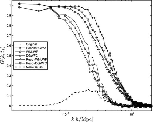
The propagator G(k, tf), defined in equation (17), which cross-correlates the initial density with the final particles’ density fields at z = 0.054. These results are carried over a single realization for clarity, and are for shown for the same combinations of techniques as in Fig. 2, with the addition of the non-Gaussian part of the WNLWF, shown with the thick dashed line.
Wavelet filtering, on the other hand, splits the field into two contributions, in such a way that the non-Gaussian features at small scales are mostly filtered out, whereas at the larger scale, those which are already Gaussian are preserved. In terms of propagator calculations, this translates in a plateau that traces the unfiltered propagator at very large scales, but then drops sooner than the original field. This loss in correlation is in fact being transferred to the non-Gaussian (filtered-out) term, and the sum of the filtered and filtered-out propagators exactly matches the original G(k). The propagator calculated with the DGWFC field also sees a slight suppression on the trans-linear regime, compared to the initial field, but weaker than the WNLWF since we are no longer filtering away information into a non-Gaussian part. In other words, the direct Gaussianization technique preserves more information about the initial field than the wavelet Wiener filter technique.
In the light of these results, however, it is legitimate to ask how much information about the BAO is preserved by the WNLWF and the DGWFC: these two techniques do indeed transform the late-time fields into Gaussian ones, but these are different Gaussian realizations than the linear evolution of the initial fields. It becomes quite delicate to interpret the results, as they still preserve most of the late-time power spectrum at large scales, they strongly correlate (>50 per cent) with the initial field up to k = 0.2 h Mpc−1 and weakly correlate (>10 per cent) down to k = 0.4 h Mpc−1. But the suppression of the propagators indicates that we are navigating away from the initial field, in a manner difficult to predict.
This raises two questions: (1) how much does this affects the final results on a cosmological analysis, and consequently (2) how much suppression is tolerable? To fully answer these questions, one needs to balance, on one hand, the gain in Fisher information about the power spectrum amplitude, and, on the other hand, the loss of information about the primordial field. Otherwise, the observed gain in Fisher information is obscured by the simple fact that we no longer know what is this informationabout?.
It turns out, as seen in Fig. 7, that the combination of reconstruction and either the WNLWF or the DGWFC has a stronger correlation to the initial field than the unfiltered one. The gain is provided by the reconstruction algorithm, and only partially ‘undone’ by the two techniques. Even if both combinations have a stronger propagator than the original field, this still brings the question whether they are outperforming the stand-alone reconstruction in the end. We therefore have no choice but to propagate the results on to a cosmological forecast, which is what we present in the next section.
Propagation on BAO
In this section, we discuss and quantify how the different Gaussianization techniques propagate on to final cosmological measurements. We recall that two competing effects are under study, and it is quite difficult to predict how they balance in detail. Let us summarize the two issues here.
All the Gaussianization techniques show a positive recovery of Fisher information about the amplitude of the power spectrum, which proves that they are indeed efficient at diagonalizing the covariance matrix. This is good news, since it represents a gain in the effective number of degrees freedom in the measurement, thereby reducing the error.
The propagator, which measures the degree of correlation between the initial density field and the final one, is affected in different ways by these techniques: the reconstruction algorithm extends the correlation to smaller scales, whereas the propagator is suppressed for both WNLWF and DGWFC. When the WNLWF and the DGWFC techniques are applied on reconstructed fields, the propagator lies about mid-way between the reconstructed and the unreconstructed fields.
We assume, for simplicity, that we are dealing with a one-dimensional measurement, i.e. s = s⊥ = s∥, and choose q = lns. However, it is straightforward to extend the formalism to the two-dimensional case, where the errors on s⊥ and s∥ are separately related to those on dA(z) and H(z), respectively.
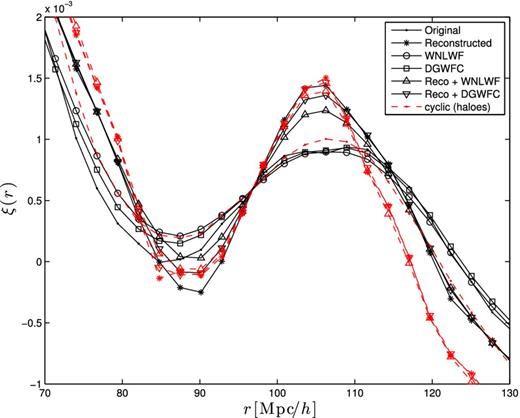
Two-point correlation function in real space, for each of the Gaussianization techniques. Different techniques recover or degrade the acoustic signal compared to the original field. This figure also serves to estimate the value of the modifier for the damping term, f, in equation (21).
We recover the expected trend that the reconstruction alone improves significantly the contrast of the BAO bump, compared to the original field. We then see that the WNLWF and the DGWFC alone both reduce the contrast, which is not desirable, but when applied on reconstructed fields, we see an overall gain in the sharpness of the peak. In the case of haloes, we find that the reconstruction technique offers a powerful gain in contrast as well, after which the two wavelet techniques have only a negligible impact.
In Fig. 9, we gather all the pieces and present the error about a BAO dilation scale measurement, for each of the techniques. We observe that the density reconstruction alone outperforms any other techniques or combinations of techniques, by a factor of 1.3–2.2. Both the WNLWF and DGWFC stand-alone techniques provide about the same constraining power as the original fields, meaning that the gain in Fisher information brought by the wavelet techniques is almost perfectly lost by the smoothing of the BAO peak. Both combined techniques offer a gain of about a factor of 1.8 compared to the original fields, but are still weaker than reconstruction alone. Similar conclusions can be reached for haloes, with the difference that the WNLWF and DGWFC have very little impact once applied on the reconstructed fields.
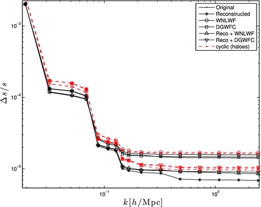
Fractional error on the BAO dilation scale, as a function of the smallest scale included in the survey. The step-like shape at low k comes from the derivative of the power spectrum in the BAO regime. Results for particles and haloes are shown with solid and dashed lines, respectively. We see from this figure that in both cases, the density reconstruction alone offers the tightest constraints on the BAO dilation scale, and that wavelet-based techniques alone degrade the constraining power by about a factor of 2.
Therefore, the gain in Fisher information does not map linearly into a gain in the BAO measurement. Instead, we observe that it can be equivalent to have a series of highly correlated measurements about a sharp BAO peak – i.e. the original fields – or a series of almost uncorrelated measurements about a smoother peak – i.e. the wavelet methods. These two competing effects (lower correlations and peak smoothing) do not always cancel out: when considering the combined techniques, the loss due to peak smoothing is not fully compensated by the gain due to lowered correlations, leading to a net degradation of constraining power on the BAO compared to reconstruction alone.
DISCUSSION AND CONCLUSION
The first part of this paper explores the recovery of Fisher information content in the amplitude of the matter power spectrum with the combined use of three Gaussianization techniques – DGWFC, wavelet non-linear Wiener filtering and density reconstruction. In the trans-linear regime, we show that it is possible to extract an order of magnitude more information by combining the reconstruction technique with one of the other two, compared to the original fields. The fact that the conjunction of two methods outperforms the performance of the individual techniques can be understood as follows: the density reconstruction first acts as to undo the large-scale gravitational infall towards the overdensities, and the wavelet filter or the Gaussianization method subsequently suppresses the residual non-Gaussian features that persist, leaving the power spectrum covariance matrix highly diagonal. The reverse order would not have performed that well, since the reconstruction technique needs an accurate measurement of the gravitational potential about the collapsed structures, a dynamical regime that is highly modified by both the wavelet non-linear Wiener filtering and the direct Gaussianization.
We also repeat these Fisher calculations on halo catalogues and find that (1) the density reconstruction recovers about two times more information by k = 0.6 h Mpc−1, compared to the original halo fields, (2) wavelet Wiener filtering is even more efficient and recovers about three times more information, (3) both of these techniques still combine well, and allow for a recovery factor of 5, and (4) direct Gaussianization generally acts as to reduce the Fisher information.
After applying a conservative shot noise subtraction technique, the Fisher information goes down significantly, but the reconstruction technique can still recover about two times more Fisher information by k > 0.6 h Mpc−1. In this simple noise modelling (Pshot = 1/n ∼ 400 h−3 Mpc3), the NLWF and the direct Gaussianization seem to bring very little benefits, at least in the regime where this toy model departs or agrees reasonably well with more sophisticated methods. However, we believe, from Fig. 3, that our noise estimate is too high, and we know from the measurements on particles that lower shot noise systems gain from our filtering technique. It seems thus that NLWF and direct Gaussianization are worth the effort in the case where shot noise is both intrinsically low and well estimated.
These results suggest that non-Gaussian error estimates about the matter power spectrum can be minimized in the trans-linear regime, a fact that directly affects the uncertainty about the BAO measurements. In other words, optimizing the recovery of Fisher information with such techniques might benefit the constraints about cosmological parameters such as dark energy equation of state.
In the second part of the paper, we investigate how these techniques influence our ability to constrain cosmology from a BAO toy analysis. Using the formalism of Eisenstein et al. (2007b), and for each of these techniques, we constructed a Fisher matrix that propagates the uncertainty from the measured power spectrum covariance matrix on to that of the BAO dilation scale. We show that in fact, the two wavelet techniques tend to smooth out the BAO bump in configuration space, which tend to weaken BAO constraints. In the end, we show that the diagonalization of the matrices provided by both the WNLWF and the DGWFC counter-balances the loss of contrast in the BAO feature, with no net gain in constraining power compared to the original fields. The wavelet techniques combined with reconstruction do lower the error bar, but not as much as the reconstruction alone. Similar results are found both with particles and haloes.
The part that is potentially confusing is that these two wavelet techniques exhibit a gain in the Fisher information; however, one needs to understand exactly what this information is about. It turns out that the gain is only about their own power spectrum amplitude, but not about that of the initial density field. On the contrary, we show that the cross-correlation between the initial and late-time fields is in fact reduced by the two wavelet techniques. We thus conclude that one should take extra care when claiming that a given technique recovers Fisher information, since the impact on the cosmological parameter constraints is not always obvious.
For the three techniques we discussed here, our results show that one should not use WNLWFor DGWFC, but only density reconstruction. To reach fully general conclusions, the analyses would need to be repeated with other transformations (i.e. log-normal, Cox–Box, etc.), and the results might be different, then. However, we strongly advise to perform propagator and toy model calculations in order to gauge the actual effect on the final product.
In this paper, we have only carried the calculations only for a BAO toy analysis; we want to stress that other cosmological analyses based on the power spectrum (neutrino mass, global shape, σ8 measurements) might actually benefit from a conjunction of two Gaussianization techniques. In the era of precision cosmology, such approaches are definitively worth trying, as they are quite easy to implement and are generally helpful in removing noise.
We would like to thank the anonymous referee for insisting on measuring the propagator, as it triggered important discussions and results. This work was supported by the National Science Foundation of China (Grant No. 11173006), the Ministry of Science and Technology National Basic Science program (project 973) under Grant No. 2012CB821804 and the Fundamental Research Funds for the Central Universities. Computations were performed on the TCS supercomputer at the SciNet HPC Consortium. SciNet is funded by: the Canada Foundation for Innovation under the auspices of Compute Canada; the Government of Ontario; Ontario Research Fund – Research Excellence; and the University of Toronto. UP would like to acknowledge NSERC for its financial support, and JHD is supported by a CITA National Fellowship.
We note that each wavelet mode has its own PDF; hence, we should really be writing |$f_{\rm PDF}^{l_1,l_2,l_3}(x)$|, but we omit the location indices to clarify the notation.
We use the same meaning for wavelet ‘mode’ as for the WNLWF case.
We used the 2011 January version of halofit, which is known to underestimate the power in the non-linear regime by 5–10 per cent. We could have used the latest version; however, it is also known to overpredict the power in LCDM universes (see Heitmann et al. 2013). In any case, the results from this paper would not be affected since we base our comparisons solely on N-body simulations.
We could of course improve the performance of the reconstruction technique by using the gravitational potential measured from simulated particles, which we have at hand. Even in a data set, it is in principle possible to combine independent measurements of the potential, obtained with weak lensing tomography for instance. This is an interesting avenue that is, however, beyond the scope of this paper.
REFERENCES
APPENDIX A: WAVELET FILTERS AND HALO DISTRIBUTIONS
In this section, we briefly comment on the non-Gaussian part of the WNLWF, which is designed to suppress the highly collapsed structures from the density fields. By looking at the filtered-out material, we expect to recover a good match with the halo distributions. This is what we present in Fig. A1. Both figures seem to correlate quite well; hence, it would be possible to use one as a proxy for the other.
Projections through a thickness of 200 cells of one of the realizations. In each panel, the side is 322.36 h−1 Mpc, and the image contains 10242 pixels. Top left shows the original particle field, top right shows the original halo field, bottom left shows the non-Gaussian part of the WNLWF field and bottom right shows the Gaussian part of the WNLWF acting on halo fields. To ease the visual comparison, each panel shows the same overdensity range and saturates for denser regions, i.e. all pixels with δ > 5 are black.
We also show the result of the WNLWF on the halo distribution, which, from Fig. 2, is closer to the linear power spectrum. The shot noise is still high, but the field clearly preserves the structures. Although there is room for improvement, we can see how techniques such as this one can help dig out the haloes from noisy density fields or reversely populate halo fields with ‘particles’ (bottom-left panel).
