


Abstract
We present a new analysis of the results of the Expérience pour la Recherche d'Objets Sombres (EROS)-2, Optical Gravitational Lensing Experiment (OGLE)-II and OGLE-III microlensing campaigns towards the Small Magellanic Clouds (SMC). Through a statistical analysis we address the issue of the nature of the reported microlensing candidate events, whether to be attributed to lenses belonging to known population [the SMC luminous components or the Milky Way disc, to which we broadly refer to as ‘self-lensing’] or to the would be population of dark matter compact halo objects (MACHOs). To this purpose, we present profiles of the optical depth and, comparing to the observed quantities, we carry out analyses of the events position and duration. Finally, we evaluate and study the microlensing rate. Overall, we consider five reported microlensing events towards the SMC (one by EROS and four by OGLE). The analysis shows that in terms of number of events the expected self-lensing signal may indeed explain the observed rate. However, the characteristics of the events, spatial distribution and duration (and for one event, the projected velocity) rather suggest a non-self-lensing origin for a few of them. In particular, we evaluate, through a likelihood analysis, the resulting upper limit for the halo mass fraction in form of MACHOs given the expected self-lensing and MACHO lensing signal. At 95 per cent CL, the tighter upper limit, about 10 per cent, is found for MACHO mass of 10−2 M⊙, upper limit that reduces to above 20 per cent for 0.5 M⊙ MACHOs.
1 INTRODUCTION
The original motivation for stellar microlensing (Paczyński 1986) is the search for dark matter candidates in form of (faint) massive compact halo objects (MACHOs) in the galactic haloes. Indeed, over a broad mass range of the putative MACHO population, our current understanding of this relevant astrophysical issue is mainly based on the results of the observational microlensing campaigns carried out to this purpose. On the other hand, the current understanding for the nature of most, if not all, dark matter at the Galactic level is from some yet undiscovered particle (Strigari 2012) (for a general discussion of dark matter and gravitational lensing, we refer to Bartelmann 2010; Massey, Kitching & Richard 2010). The probability for a microlensing event to occur is extremely small. This is described in terms of the microlensing optical depth which is of the order of 10−6 or smaller [we refer to Mao (2012) and references therein for an updated introduction to microlensing]; therefore, dense stellar fields have to be monitored to increase the rate of events. Microlensing campaigns for the search of MACHOs have been carried out towards the Magellanic Clouds (Moniez 2010) and M31 (Calchi Novati 2010). Besides the dark matter issue, meanwhile microlensing has become an established tool for analyses of stellar astrophysics (Gould 2001) and, through observations towards the Galactic bulge, for the search of extra-solar planets (Dominik 2010).
The Magellanic Clouds (Large and Small), located within the Galactic halo, are privileged targets for the search of microlensing events. Up to now about 20 candidate events have been reported towards these lines of sight and important, though not always coherent, results have been reported. There is an agreement to exclude MACHOs as viable dark matter candidates for masses below ≈(10−1 − 10−2) M⊙ (down to about 10−7 M⊙). Some debate remains in the mass range (0.1–1) M⊙ where, according to some observational outcomes, a sizeable fraction, if not most of the halo mass, may indeed be in form of compact halo objects. For larger values of the MACHO mass (where the expected number of events decreases), the limits obtained with microlensing analyses are weaker than with other techniques (Yoo, Chanamé & Gould 2004; Quinn et al. 2009; Quinn & Smith 2009); in this mass range, it appears to be useful also to consider the cross-matching of microlensing with X-ray catalogues (Sartore & Treves 2010, 2012). The event duration, the ‘Einstein time’ tE, the main physical observable for microlensing events, is driven by the lens mass, m, scaling as |$\sqrt{m}$| (though it also depends on other non-directly observable quantities as the lens–source relative transverse velocity and the lens and source distances). A possibly non-exhaustive list of potential lens populations, to which we broadly refer to as ‘self-lensing’ as opposed to MACHO lensing populations, includes lenses belonging to the luminous components of the Small Magellanic Cloud (SMC), which act also as sources, and the disc of the Milky Way (MW; in fact, we will consider also non-luminous lenses belonging to these populations moving down to the substellar mass range to include also brown dwarfs). The suggestion that the events observed towards the Magellanic Clouds may not be due to MACHOs dates back at least to the analyses of Sahu (1994), Wu (1994), Gould (1995) and has been thereafter the object of several analyses (Salati et al. 1999; Di Stefano 2000; Evans & Kerins 2000; Gyuk, Dalal & Griest 2000; Jetzer, Mancini & Scarpetta 2002). It is therefore relevant to reliably determine the signal expected from self-lensing lens populations as compared to that of MACHO lensing.
More specifically, the MACHO Collaboration claimed for a mass halo fraction in form of ∼0.5 M⊙ MACHOs of about f ∼ 20 per cent out of observations of 13–17 candidate microlensing events towards the LMC (Alcock et al. 2000), a result further discussed in Bennett (2005) where in particular the microlensing nature of 10–12 out of the original set of 13 candidate events has been confirmed. On the other hand, in disagreement with this result, the analyses of the Expérience pour la Recherche d'Objets Sombres (EROS; Tisserand et al. 2007) and the Optical Gravitational Lensing Experiment (OGLE) collaborations, for both OGLE-II (Wyrzykowski et al. 2009, 2010) and OGLE-III (Wyrzykowski et al. 2011a,b), out of observations towards both the LMC and SMC, concluded by putting extremely severe upper limits on the MACHO contribution also in this mass range. In particular, at 95 per cent CL, the EROS Collaboration reported an upper limit f = 8 per cent for |$0.4\,\rm {M}_{\odot }$| MACHOs, and OGLE f = 6 per cent for |$0.4\,\textrm {M}_{\odot }$| MACHOs and f = 4 per cent in the mass range between 0.01 and |$0.15\,\textrm {M}_{\odot }$|.
Rather than addressing, as we also mainly do in this work, the issue on the lens nature, whether self-lensing or MACHO lensing, one may also consider different source populations which may possibly enhance the microlensing rate (see for instance Rest et al. (2005) and reference therein for a broad overall discussion of the different possible source and lens populations). For the specific case of the LMC, recently Besla, Hernquist & Loeb (2013) proposed, as possible sources, a SMC stripped population (still to be observed, though) lying behind the LMC, which may explain simultaneously both the MACHO and the OGLE observational results towards the LMC [see however Nelson et al. (2009) who, on a general ground, concluded against the possibility for the sources to lie behind the LMC].
With respect to the LMC, the case of the SMC is somewhat peculiar. As further discussed below, the SMC is quite elongated along the line of sight. As the microlensing cross-section, the Einstein radius, is proportional to the (square root of) the source–lens distance, an elongated structure is expected to enhance the SMC self-lensing signal. As a result, the ratio of self-lensing versus MACHO lensing (if any) is larger than towards the LMC making overall more difficult to disentangle the two signals and to draw stringent conclusions on the issue of MACHOs. On the other hand, the characteristics that differentiate the two lines of sight can be considered as a strength when cross-matching the results.
In previous analyses, we have addressed the issue of the nature of the reported events towards the LMC by the MACHO (Mancini et al. 2004; Calchi Novati et al. 2006) and the OGLE collaborations (Calchi Novati et al. 2009; Calchi Novati & Mancini 2011). In this paper, we report a detailed analysis of the EROS and the OGLE observational campaigns towards the SMC (as further discussed below, we do not include data from the observational campaign carried out by the MACHO Collaboration along this line of sight). The underlying idea behind our approach is to characterize statistically, starting from a reliable model for all possible lens populations, the observed versus the expected signal in order to address the issue of the nature of the reported microlensing candidate events. First, we evaluate profiles of the optical depth, in particular for SMC self-lensing. This tells us how the SMC structure is reflected in the expected microlensing signal and carries information on the overall spatial density of the given lens population. To include within the analysis the specific characteristics of the observed events, in particular number, position and duration, we carry out an investigation based on the microlensing rate which then allows us to derive limits on the halo mass fraction in form of MACHOs.
The plan of the paper is as follows. In Section 2, we describe the models used in our analysis, with a particular attention to the SMC structure. In Section 3, we resume the status and the results of previous and ongoing microlensing campaign towards the SMC. In Section 4, we present our analysis. In Section 4.1, we present the profiles of the optical depth. In Section 4.2, we introduce the microlensing rate, our main tool of investigation. In Section 4.3, we derive the expected microlensing quantities, number of events and duration. In Section 4.4, we address the issue of the possible nature of the reported observed events and in particular we evaluate the limits on dark matter in form of compact halo objects. In Section 5, we compare our results to previous ones towards the SMC and critically analyse, as for the search of MACHOs, the line of sight towards the SMC against that towards the LMC. Finally, in Section 6, we present our conclusions.
2 MODEL
The microlensing quantities, the microlensing optical depth and the microlensing rate, depend on the underlying astrophysical model. In particular, the optical depth depends uniquely on the lens (and source) population spatial density, whereas the microlensing rate depends also on the lens mass function and the lens–source relative velocity. Indeed, for the more common situation of a point-like single lens and source with uniform relative motion, the only physical observable characterizing the events is the Einstein time, tE, which is a function of the lens mass, the lens–source relative velocity and the lens and source distances. None of these quantities, however, is directly observable. The underlying astrophysical models are therefore essential to assess the characteristics of the expected signal from all the possible lens populations. In the present case: self-lensing, which fixes the background level, and MACHO lensing, the ‘signal’ we want to constraint.
In the following analysis we consider, as possible lens populations, SMC and MW stars (and brown dwarfs), both contributing to the self-lensing signal, and the would-be population of compact halo objects in the MW halo, which we describe in turn.
2.1 The SMC: structure and kinematics
2.1.1 Structure
The SMC is a dwarf irregular galaxy orbiting the MW in tight interaction with the (larger) LMC (van den Bergh 1999; McConnachie 2012). Also because of this complicated dynamical situation, the detailed spatial structure and overall characteristics of the SMC are still debated. For the overall SMC stellar mass, which is a quantity of primary importance to our purposes, being in the end (almost) directly proportional to the SMC optical depth and number of expected events, we use M* = 1.0 × 10⁹ M⊙ (within 5 kpc of the SMC centre), which is the value of the ‘fiducial’ model of Bekki & Chiba (2009) (see also Yoshizawa & Noguchi 2003). According to reported values of the SMC luminosity, this correspond roughly to a mass-to-light ratio within the range M/LV ∼ 2–3. We recall that McConnachie (2012) reports M* = 4.6 × 10⁸ M⊙, which is half smaller than our fiducial value, and that Bekki & Stanimirović (2009), for a stellar luminosity 4.3 × 10⁸ L⊙, consider the ‘reasonable’ range for the mass-to-light ratio to be M/LV ∼ 2-4, depending in particular on the fraction of the old stellar population. In a previous work, Stanimirović, Staveley-Smith & Jones (2004), for a stellar luminosity 3.1 × 10⁸ L⊙, estimated a total stellar mass of the SMC 1.8 × 10⁹ M⊙ (within 3 kpc of the SMC centre). Overall, the systematic uncertainty on this relevant quantity we find in literature is of about a factor of 2.
The total dynamical mass of the SMC has also been the object of several investigations. Stanimirović et al. (2004) report 2.4 × 10⁹ M⊙ within 3 kpc, a result confirmed in Harris & Zaritsky (2006) who report values in the range 1.4–1.9 × 10⁹ M⊙ within 1.6 kpc and a less well constrained mass within 3 kpc between 2.7 and 5.1 × 10⁹ M⊙. These values therefore suggest the existence of a dark matter component even in the innermost SMC region, as thoroughly discussed in Bekki & Stanimirović (2009).
According to the star formation history of the SMC (Harris & Zaritsky 2004), we can broadly distinguish two components: an old star (OS) and a young star (YS) population. Several analyses have shown that indeed, besides their age, these populations also show different morphology structures. We base our analysis upon the recent work of Haschke, Grebel & Duffau (2012), which in turn is based on the OGLE-III SMC variable stars data but see also, among others, Kapakos, Hatzidimitriou & Soszyński (2011), Kapakos & Hatzidimitriou (2012), Nidever et al. (2011), Subramanian & Subramaniam (2009, 2012). In particular, Haschke et al. (2012) address the issue of the three-dimensional SMC structure based on the analysis of RR Lyrae stars and Cepheids as tracers of the old and young populations, respectively. Haschke et al. (2012) report estimates for the position and the inclination angles and for the line-of-sight depth which is a crucial quantity for microlensing purposes as the microlensing cross-section, and in the end the microlensing rate, grows with the lens–source distance, so that a large SMC intrinsic depth enhances the SMC self-lensing signal whereas, on the other hand, the details of the inner SMC structure are not essential to determine the expected lensing signal for the MW lens populations (Section 4.1). Moreover, Haschke et al. (2012) show contour plots for the stellar density of RR Lyrae stars and Cepheids not only on the plane of the sky but also on the distance–declination and the distance–right ascension planes. For fixed values of the position and inclination angles and line-of-sight depth, we therefore build our model trying to broadly match this full three-dimensional view of the SMC.
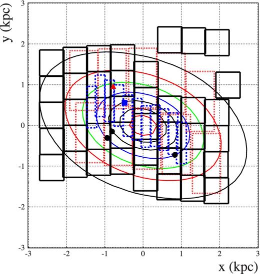
The fields of view monitored towards the SMC projected on the plane of the sky by OGLE-II (dashed lines, 11 fields), OGLE-III (solid lines, 41 fields) and EROS-2 (dotted lines, 10 fields). The position of the five reported candidate events is also included: one for OGLE-II (square), three for OGLE-III (circles) and one for EROS-2 (triangle). Further details on the events are given in Table 1. Also reported, the projected density for our fiducial SMC model (Section 2). The contours shown correspond to the values 0.2, 0.4, 0.6, 0.8, 1.0, 1.2, 1.4 in units of 108 M⊙ kpc−2. The x-y reference system has its origin at the centre of the SMC, the x-axis antiparallel to the right ascension and the y-axis parallel to the declination.
The centre and the distance of the SMC are both not too well constrained and in particular an offset of the young and old population, both in distance and in position, which may indeed be relevant for the evaluation of the microlensing quantities, has been discussed by several authors. Here again we follow the analysis of Haschke et al. (2012), and reference therein, and assume, for our fiducial model, the same centre and distance for both populations. In particular, we choose the optical centre reported by Gonidakis et al. (2009) α = 0h51m and δ = −73| $_{.}^{\circ}$|1 (J2000) and a distance to the SMC of 61.5 kpc, the median distance of RR Lyrae stars (Haschke et al. 2012) found in agreement with that of the Cepheids. Finally, we fix the tidal radius of the SMC at 12 kpc.
Because of a relative shift in distance between the OS and YS populations is still compatible with the data and may be expected to enhance the microlensing rate, as a test model we consider the case where the centre of the YS population is shifted by 2 kpc behind that of the OS one, at 63.5 kpc, rescaling (increasing) the YS axes ratio to keep the same shape on the plane of the sky and changing accordingly the central normalization.
In Palanque-Delabrouille et al. (1998), the EROS Collaboration introduced an SMC model for an estimate of the SMC self-lensing optical depth which has therefore become an often quoted ‘fiducial’ value for this quantity. The SMC, for a total stellar mass of ∼1 × 10⁹ M⊙ (a value that matches the one we use in our model), is approximated with a single population prolate ellipsoid elongated along the line of sight with exponential profile. The radial scalelength, transverse to the line of sight, is fixed at 0.54 kpc and the scaleheight along the line of sight is left free to vary in the range 2.5–7.5 kpc. We recall that the scaleheight is smaller than the depth by a factor 0.4648 (Haschke et al. 2012), so that 2.5 kpc is the value that better matches our ones. Although clearly disfavoured, in view of the more recent pieces of observational evidence, we consider useful to compare to this model in consideration of its importance in the microlensing literature. Indeed, being peculiarly different but still characterized by the same overall quantities (in particular, stellar mass and scaleheight), it represents a useful test case against our fiducial model.1
2.1.2 Kinematics
We consider the velocity of SMC lenses as due to the sum of a non-dispersive component and a dispersive component. For the systemic proper motion, we follow the analysis of Kallivayalil, van der Marel & Alcock (2006) with (μW, μN) = (−1.16, −1.17) mas yr−1 (in acceptable agreement with the outcome of the analysis of Piatek, Pryor & Olszewski 2008), with an observed line-of-sight velocity 146 km s−1 (Harris & Zaritsky 2006). For the YS population, we also introduce a solid body rotation around the ξ axis (Section 2.1.1) linearly increasing up to 60 km s−1 with turnover radius at 3 kpc (Stanimirović et al. 2004). For the dispersive velocity component, we assume an isotropic Gaussian distribution [Harris & Zaritsky (2006) report the line-of-sight velocity distribution to be well characterized by a Gaussian with a velocity dispersion profile independent from the position]. For the velocity dispersion values we, again, follow those of the fiducial model of Bekki & Chiba (2009), with σ = 30 and 20 km s−1 for the old and YS populations, respectively. This is in good agreement with σ = 27.5 km s−1 for the old populations stars analysed in Harris & Zaritsky (2006) and with the analysis of Evans & Howarth (2008).
2.2 The MW disc and dark matter halo
For the MW disc, with assumed distance from the Galactic Centre 8 kpc and local circular velocity 220 km s−1 (in agreement, for instance, with the recent analysis of Bovy et al. 2012), we closely follow the analysis in Calchi Novati & Mancini (2011) with double exponential profiles thin and thick disc components with, respectively, local density 0.044 (0.0050) M⊙ pc−3, scaleheight 250 (750) pc, scalelength 2.75 (4.1) kpc (Kroupa 2007; Juric et al. 2008; de Jong et al. 2010) and line-of-sight dispersion of 30 (40) km s−1.
For the Galactic dark matter halo, in order to coherently compare with previous microlensing analyses, we assume the ‘standard’ Alcock et al. (2000) pseudo-isothermal spherical density profile with core radius 5 kpc (de Boer et al. 2005; Weber & de Boer 2010) and Alcock et al. (2000) central density 0.0079 M⊙ pc−3 (in excellent agreement with up-to-date estimates as in Bovy & Tremaine (2012), see however Garbari et al. 2012) for an isotropic Gaussian distribution velocity with line-of-sight dispersion 155 km s−1.
2.3 Mass function
For all the self-lensing populations, we assume a power-law mass function (dN/dM ∝ M−α). For MW disc lenses, following Kroupa et al. (2011), we assume slopes 1.3 and 2.3 in the mass ranges (0.08–0.5), (0.5–1) M⊙, and a present-day mass function slope 4.5 above 1 M⊙. As un upper limit for the stellar mass, which we use to normalize the mass function to match the value of the mass of the lens population (Jetzer et al. 2002), we use 120 M⊙. For the SMC YS population, we make use of the results presented in Kalirai et al. (2013) where the initial mass function of the SMC is evaluated using ultradeep Hubble Space Telescope imaging in the outskirts of the SMC (along the line of sight of the foreground globular cluster 47 Tuc). In particular, Kalirai et al. (2013) conclude for a mass function well represented by a single power-law form with slope |$1.90^{+0.15}_{-0.10}$| in the mass range (0.37–0.93) M⊙, with also indications of a turnover at the low-mass end which would not be reproduced by the same power-law index. Finally, we extend the Kalirai et al. (2013) mass function in the mass range (0.37–1.00) M⊙ and use the disc Kroupa et al. (2011) otherwise. The upper limit of integration for the lens mass within the evaluation of the microlensing rate is in principle set so to avoid any possible ‘visible’ lens. As for SMC lenses, above 1 M⊙, however, because of the extreme steepness of the mass function in this mass range, the exact value turns out to be in fact irrelevant in view of the calculation of the relevant microlensing quantities (expected number and duration of events). To be fixed, we choose for this parameter the value 2 M⊙. The microlensing results are on the other hand more sensitive to the value of this threshold for possible nearby MW lenses, given also the rapid variation of the mass–magnitude relationship with the lens distance. As a very conservative choice, intended to provide an upper limit for the expected microlensing signal of this population, we set the same value as for SMC lenses with the caveat that, reducing this threshold to 1 M⊙, the related expected signal would reduce of about 10 per cent. Given that (Section 4.3) the expected MW signal represents about 10–20 per cent of that of SMC lenses, the impact of this choice remains small. For the SMC OS population we use, following the results obtained for the Galactic bulge (Zoccali et al. 2000), a power law with slope 1.33 in the range (0.08–1) M⊙, with upper limit for integration and normalization also fixed at 1 M⊙. Besides the MW and SMC stellar populations, we also include a brown dwarf component, in the mass range 0.01-0.08 M⊙ with power-law mass function index 0.3 (Allen et al. 2005; Kroupa et al. 2011). Following the local analysis of Chabrier (2003), we attribute to this component 5 per cent of the overall relative stellar mass component.
For dark matter halo lenses, we test a series of delta mass function in the mass range 10−5–102 M⊙.
3 MICROLENSING TOWARDS THE SMC: THE EROS AND THE OGLE CAMPAIGNS
Microlensing observational campaigns towards the SMC have been carried out by the MACHO, the EROS and the OGLE collaborations. In Fig. 1, we show the monitored fields of view and the reported candidate events included in the present analysis.
The EROS Collaboration, with the EROS-2 set-up, observed a field of view covering the innermost 9 deg2 of the SMC during about 7 years from 1996 to 2003. The first results of this campaign are discussed in Palanque-Delabrouille et al. (1998), with the presentation of a long-duration event, EROS2-SMC-1, tE ∼ 120 d, which was argued to be due, also because of the lack of any parallax signal (Gould 1992) either by a large-mass object in the Galaxy halo or by a lens lying near the source in the SMC itself. The event optical depth was estimated to be compatible with that expected by SMC self-lensing. This event, first reported by the MACHO Collaboration (Alcock et al. 1997) and known as MACHO 97-SMC-1, has been the object also of a spectroscopic analysis (Sahu & Sahu 1998) whose conclusions as for the nature of the lens, based on the lack of any signal from the lens, excluded it from being an MW disc star, are in agreement with those presented in the original EROS analysis. A second analysis of this SMC EROS-2 campaign, for 5 years of data, was then presented in Afonso et al. (2003) with the inclusion of three additional long-duration candidate events claimed however to be doubtful, and finally rejected in the definite analysis presented in Tisserand et al. (2007) where only EROS2-SMC-1 was retained as a reliable candidate event (and with the analysis of Assef et al. (2006) further favouring the SMC self-lensing interpretation of this event). In their final analysis on the MACHO issue out of observations towards both Magellanic Clouds (Tisserand et al. 2007), the EROS Collaboration restricted the number of sources to a subset of ‘bright’ source objects to better address the issue of blending. Overall, the EROS-2 SMC campaign lasted Tobs = 2500 d with an estimated total number of 0.86 × 10⁶ monitored sources. With no candidate events reported towards the LMC, Tisserand et al. (2007) consider the observed rate compatible with the expected self-lensing signal and get to strong constraints on the halo mass fraction in form of MACHOs.
The OGLE Collaboration is monitoring the SMC for microlensing events since more than 15 years. Wyrzykowski et al. (2010) reported results out of the OGLE-II campaign, (1996–2000), covering the SMC innermost 2.4 deg2 for a total duration Tobs = 1408 d. The OGLE Collaboration makes the distinction between a larger sample of ‘All’ and a restricted one of ‘Bright’ sources, the latter chosen so to reduce the impact of blending in the analysis (for a discussion of the observational strategy of OGLE, in particular as for the choice of the source sample, we refer to Calchi Novati & Mancini 2011). OGLE reports an estimated number of potential sources N = 3.6 × 10⁶ (N = 2.1 × 10⁶), for the All (Bright) sample, respectively. Although Wyrzykowski et al. (2010) discuss in general terms the analyses for both samples of sources, they specifically report the results for the All sample only. Accordingly, this is the only one, we will include within our analysis for OGLE-II. In particular, Wyrzykowski et al. (2010) report a single-candidate event, OGLE-SMC-01, which is considered compatible, based on the optical depth, with the expected self-lensing signal. Thanks to an updated set-up, a much larger SMC field of view, 14 deg2, was monitored during the OGLE-III phase (2001–2009). The results of this analysis are discussed in Wyrzykowski et al. (2011b). The observational campaign lasted Tobs = 2870 d with an estimated number of sources equal to N = 5.97 × 10⁶ (N = 1.70 × 10⁶) for the All (Bright) sample, respectively. Three additional microlensing events are reported, OGLE-SMC-02, OGLE-SMC-03 and OGLE-SMC-04 (with OGLE-SMC-03 belonging to the All sample only), with the total optical depth still estimated to be in agreement with that expected from SMC self-lensing.
Among the OGLE-III SMC candidate events, OGLE-SMC-02 (also known as OGLE-2005-SMC-1) deserved special attention. This was alerted by the OGLE-III Early Warning System (Udalski 2003) and enjoyed additional observations also from space, with Spitzer, used to break the model degeneracies and solve the event, with the specific aim to measure the microlensing parallax (Dong et al. 2007). Dong et al. (2007) address in particular the issue of the nature of the lens and conclude that the most likely location is the Galactic halo from a (binary2) black hole with a total mass of around 10 M⊙.
For the EROS-2, OGLE-II and OGLE-III analyses the source number is reported per field, with 10, 11 and 41 fields monitored by each experiment, respectively. In the following, we do not include the field 140 of the OGLE-III campaign, the isolated field in the north-west part of Fig. 1, which presents a strong overdensity of (potential lens) stars being centred along the line of sight of the foreground 47 Tuc (NGC 104) globular cluster. Both EROS (Tisserand et al. 2007) and OGLE (Wyrzykowski et al. 2010, 2011b) carry out an analysis of their detection efficiency based on the estimated number of monitored sources and presented in terms of the event duration, |${\cal {E}} = {\cal {E}}(t_\mathrm{E})$|, which we also include in our analysis. In particular, OGLE reports the estimate for the efficiency both for a ‘sparse’ and a ‘dense’ field, depending on the density of stars. Accordingly, for each given value of the duration, we linearly interpolate the efficiency taking into account the estimated number of sources per field (the same value we use to estimate the expected number of events), while keeping the reported values as fixed for those fields with lower, respectively higher, source star number. (This expedient, however, is effective for OGLE-II only, as for OGLE-III the available data for the sparse and dense fields indicate that the efficiency is roughly constant across the overall monitored field of view, even though the choice of the, two nearby, fields used for this analysis by OGLE-III may have biased this outcome.) In Fig. 2, we report a detail of the efficiency function |${\cal {E}}(t_\mathrm{E})$| for tE < 200 d. Besides the dependence on the crowding, we remark the low maximum value of |${\cal {E}}(t_\mathrm{E})$| for OGLE-II as compared to those of OGLE-III and EROS-2 and, for EROS-2, the much faster increase up to rather large values for small durations as compared to OGLE.
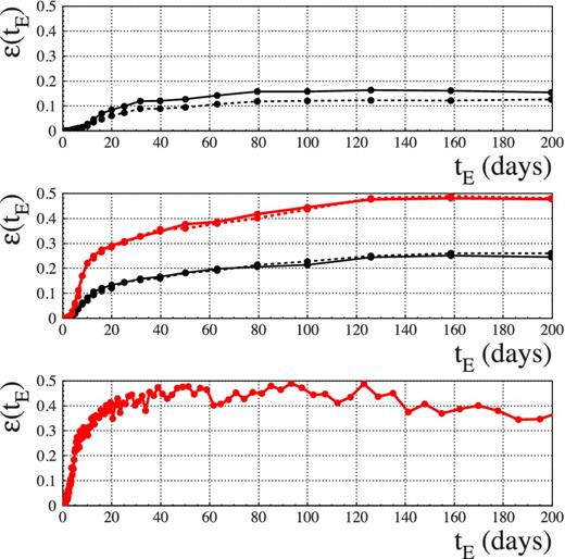
The detection efficiency as a function of the duration, |${\cal {E}}(t_\mathrm{E})$|, for OGLE-II (top panel, All sample), OGLE-III (middle panel) and EROS-2. For OGLE the solid and dashed curves trace the efficiency for ‘sparse’ and ‘dense’ fields, as a measure of the crowding, respectively (for OGLE-III the two curves are almost indistinguishable). For OGLE-III, the thicker curves (with larger values of the efficiency) refer to the Bright sample of sources.
Overall, there are five microlensing candidate events reported towards the SMC upon which EROS and OGLE based their analyses and whose characteristics we summarize in Table 1 and which we will further consider in the present analysis. For definiteness, we will consider as homogeneous the All sample of sources of OGLE-II and OGLE-III and the Bright sample of sources of OGLE-III together with that of EROS-2.
Microlensing candidate events for the OGLE-II, OGLE-III and EROS-2 observational campaigns towards the SMC. The values for the duration, which are those used for the present analysis, and the estimate for the optical depth are from Wyrzykowski et al. (2009), Wyrzykowski et al. (2011b) and Tisserand et al. (2007), respectively. The coordinate positions are expressed in terms of the reference frame used in Fig. 1.
| Event | x | y | tE | τ |
|---|---|---|---|---|
| (kpc) | (kpc) | (d) | [10−7] | |
| OGLE-SMC-01 | −0.485 679 | 0.555 917 | 65.0 | 1.55 |
| OGLE-SMC-02 | 0.831 350 | −0.725 003 | 195.6 | 0.85 |
| OGLE-SMC-03 | −0.937 994 | −0.309 247 | 45.5 | 0.30 |
| OGLE-SMC-04 | −0.812 418 | −0.150 195 | 18.60 | 0.15 |
| EROS2-SMC-1 | −0.781 914 | 0.966 178 | 125. | 1.7 |
Besides EROS and OGLE, also the MACHO Collaboration monitored the SMC for microlensing events. The microlensing event MACHO Alert 98-SMC-1 has been the first binary caustic crossing event reported towards the Magellanic Clouds (Alcock et al. 1999), also monitored by the PLANET Collaboration (Rhie et al. 1999). The analysis of the event, including additional data from the EROS and the OGLE data base, and in particular of the lens projected velocity, led to the conclusion that the event is more likely to reside in the SMC than in the Galactic halo (Alcock et al. 1999; Albrow et al. 1999; Rhie et al. 1999). The MACHO Collaboration, however, did not present a detailed and complete analysis of the SMC campaign, as they did for the LMC one. In particular, the estimate of the number of sources and the analysis of the detection efficiency, essential information to reliably assess the characteristics of the expected signal, are both missing. For this reason hereafter we no longer consider the results of the MACHO Collaboration campaign towards the SMC.
4 ANALYSIS
4.1 The microlensing optical depth
According to its definition as an instantaneous probability, τ is a static quantity which cannot be used to characterize the observed events. This feature makes the optical depth a very useful quantity from a theoretical point of view, being less model dependent, but also observationally. An estimate of the measured optical depth can indeed be used to trace the underlying mass (and spatial) density distribution of a given lens population.
Coming to the specific problem of SMC microlensing, also looking at equation (4), we expect the signal from the MW lens populations to be rather independent from the inner structure of the SMC (with ρl ≈ 0 within the SMC where ρs ≠ 0). It results,4 in particular, that the profiles for the MW disc and the Galactic halo optical depth are roughly constant across the field of view. Specifically, for the MW halo profile τ ∼ 6.3 × 10⁻⁷ (for a full MACHO halo) and for the MW disc τ ∼ 0.04 × 10⁻⁷, in both cases with relative variations up to 5 per cent level. The SMC self-lensing optical depth, on the other hand, following the underlying lens spatial density profile, is strongly variable, Fig. 3, with peak central value, for our fiducial model, τ = 1.3 × 10⁻⁷, and the observed events falling within the lines of equal optical depth values 0.5 and 0.8 × 10⁻⁷. As expected, the introduction of a shift in distance between the OS and the YS population for a test model against the fiducial one (Section 2.1.1) enhances the SMC self-lensing signal. The relative increase with respect to the fiducial model is at 6 per cent level at the SMC centre and below 5 per cent for the average values across the monitored fields of view (in particular, with the YS lying 2 kpc behind the OS, there is a strong enhancement, about 80 per cent, of the signal from YS sources with OS lenses, which is however almost completely compensated by a corresponding decrease in the signal from OS sources with YS lenses). For completeness, we mention also the outcome of the optical depth analysis for the SMC dark matter halo. The profile is asymmetric following the underlying SMC luminous profile and overall inclination, with, for a full SMC halo, peak value 0.46 × 10⁻⁷ (in the south-west part of the SMC, following the SMC inclination, around at position x, y = 1.1, −0.6 in the reference frame of Figs 1 and 3) and average value across the field of view in the range (0.31-0.38) × 10− 7 (the smaller and larger value for OGLE-III and OGLE-II fields, respectively). Overall, this is only about 5 per cent of the MW halo signal and therefore we will hereafter neglect this component.
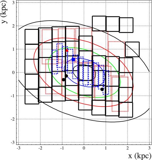
SMC self-lensing optical depth profile. The contours shown correspond to the values 0.1, 0.3, 0.5, 0.8, 1.0 in units of 10−7. The maximum value is 1.3 × 10⁻⁷. The reference system, the observed event positions and field contours are indicated as in Fig. 1.
The MW dark matter halo optical depth we evaluate towards the SMC for a full MACHO halo, 6.3 × 10⁻⁷, is significantly larger than the corresponding value we had evaluated towards the LMC, 4.5 × 10⁻⁷ (Calchi Novati et al. 2009). This increase is to be attributed to the increase in Galactic longitude and, to somewhat less extent, to the increase of the distance (whereas the increase, in absolute value, in Galactic latitude tends to reduce the optical depth).
In the following, we will address the issue of the nature of the observed events through the analysis of the microlensing rate. It is however useful to consider, to some extent, this issue already within the framework of the optical depth, in particular asking whether the stellar lens populations may or may not explain the observed signal and this starting from the consideration that the largest signal is expected, as it may be guessed looking at the relative values of the optical depth, from stellar lenses within the SMC rather than from MW disc lenses.
The expected quantity to be compared to the measured optical depth is the average optical depth value across the field of view where the Nobs source stars entering equation (5) are monitored. Furthermore, as to be expected and according to equation (6), the relative (statistical) error on this estimate scales with the (square root of the) number of observed events and in particular σ(τ)/τ = 1 for Nev = 1. To draw robust conclusions based on the optical depth, being statistical statements, a large enough sample of observed events is therefore mandatory.
The average optical depth for SMC self-lensing across the monitored fields of view, according to our fiducial model, is 〈τexp〉 = 0.50, 0.81 and 0.39 (in units of 10−7) for EROS-2, OGLE-II and OGLE-III, respectively. This quantity is to be compared with the values already reported in Section 3. For EROS-2 and OGLE-II, with a unique event (and always in units of 10−7) τobs = 1.7 ± 1.7 (EROS-2) and 1.55 ± 1.55 (OGLE-II) and τobs = 1.30 ± 1.01 for OGLE-III with three reported events. Although larger, the observed values are, within their large error, easily in agreement with the expected ones for SMC self-lensing.
We can compare these results with those reported in the analysis of Palanque-Delabrouille et al. (1998), as for the SMC self-lensing signal, often quoted and used as a ‘fiducial value’. In particular, for a scalelength h = 2.5 kpc, Palanque-Delabrouille et al. (1998) report, for SMC self-lensing, an average value of 1.0 × 10⁻⁷. Allowing for the caveat of the different central normalization (Section 2.1), possibly because of a different definition of the region over which we average the optical depth and/or for a difference in other parameters of the model, we fail to reproduce this result. With a peak central value of 6.2 × 10⁻⁷ we find instead an average expected value of 0.8 × 10⁻⁷ for the EROS-2 monitored fields of view. For OGLE-II and OGLE-III, we obtain 1.7 and 0.56 × 10⁻⁷, respectively. Comparing with the results of our fiducial model, following also the discussion in Section 2.1, we find that this density distribution leads to a much more centrally peaked optical depth profile (with the larger relative difference for the OGLE-II fields).
The SMC self-lensing optical depth has been analysed also by other authors. Sahu & Sahu (1998) estimate values in the range 1.0-5.0 × 10− 7. Graff & Gardiner (1999), based on the Gardiner & Noguchi (1996) N-body simulation of the SMC, derived an average smaller value, 0.4 × 10⁻⁷, arguing that, compared to the Palanque-Delabrouille et al. (1998) and Sahu & Sahu (1998), both reporting larger values, a reason of disagreement could be traced back in the smaller line-of-sight thickness used. All these analyses, however, somehow suffer from the very large uncertainties in the model of the SMC luminous components which, if not still fully solved, are by now largely smoothed out by the more recent analyses (as in particular those based on the newly available OGLE-III data set).
4.1.1 The SMC self-lensing optical depth: a spatial distribution analysis
Given the very small number of observed events we cannot aim at drawing stronger conclusions on the basis of the optical depth analysis. We can still, however, try to gain some further insight by addressing the issue of the spatial distribution of the events. The motivation comes from the observation of the very rapid, non-linear, variation of the expected optical depth profile across the monitored fields of view (which is made apparent, for instance, by the strong decrease of the expected average value moving from OGLE-II to OGLE-III, where a much larger region has been monitored). This makes the average optical depth value reported above of limited interest. The usual way out to address this issue is to consider smaller and more homogeneous subregions where to perform the analysis.
Our choice is to fix the bin size by asking that each bin contain the same number of monitored source stars (this is suggested by equation (5) according to which, once fixed the observed events, the estimate of the observed optical depth scales as 1/Nobs). Specifically, we choose to select four bins whose exact extension varies according to the different set-up we consider (EROS-2, OGLE-II and OGLE-III). The values of the average expected optical depth for SMC self-lensing within the bins are reported in Table 2 (for convenience all the values are divided by a factor 4 so that they can be directly compared to the already reported observed values, as each bin contains exactly 1/4 of the total number of monitored sources). The data in Table 2 allow us to better quantify the variation of the optical depth across the monitored field of views shown in Fig. 3. In particular, we note the much stronger gradient expected with the Palanque-Delabrouille et al. (1998) model as compared to the smoother fiducial one. Additionally, we can trace the position of the observed events within this parameter space, providing us with a more quantitative hint on their spatial distribution (a larger set of events would then allow one to carry out a more robust analysis by comparing the observed to the expected profile of the optical depth). In particular, it results that, moving from the outer bin inwards, both the EROS-2 and OGLE-II events fall within the second bin (which, especially for the second event, at glance from Fig. 3 is not apparent) whereas all the three OGLE-III events fall within the third bin (the corresponding values are underlined in Table 2), therefore in a more central position.
Expected average values for the SMC self-lensing optical depth within the bins of the spatial distribution analysis. In columns (1–3) and (4–6), we report the results for the fiducial and the Palanque-Delabrouille et al. (1998) models, respectively. In particular, we report the results for EROS-2, columns (1) and (4); OGLE-II, columns (2) and (5); OGLE-III, columns (4) and (6). The observed event(s) for each data set fall within the bin whose expected value is underlined. The reported values are normalized so that they are homogeneous to the observed values reported in Table 1 (see the text for further details).
| Bin | (1) | (2) | (3) | (4) | (5) | (6) |
|---|---|---|---|---|---|---|
| 1 | 0.08 | 0.17 | 0.06 | 0.06 | 0.19 | 0.03 |
| 2 | 0.13 | 0.21 | 0.11 | 0.15 | 0.43 | 0.12 |
| 3 | 0.17 | 0.24 | 0.17 | 0.31 | 0.65 | 0.27 |
| 4 | 0.22 | 0.28 | 0.24 | 0.55 | 0.96 | 0.65 |
| Bin | (1) | (2) | (3) | (4) | (5) | (6) |
|---|---|---|---|---|---|---|
| 1 | 0.08 | 0.17 | 0.06 | 0.06 | 0.19 | 0.03 |
| 2 | 0.13 | 0.21 | 0.11 | 0.15 | 0.43 | 0.12 |
| 3 | 0.17 | 0.24 | 0.17 | 0.31 | 0.65 | 0.27 |
| 4 | 0.22 | 0.28 | 0.24 | 0.55 | 0.96 | 0.65 |
For the above discussion on the spatial distribution we have considered, for self-lensing, the SMC luminous component lenses only. This is justified by the much larger optical depth of this component compared to that of MW disc lenses. Specifically, the ratio of the optical depth average value for SMC self-lensing over that of MW disc vary in the range from ∼10 up to ∼20 (for OGLE-III and OGLE-II fields, respectively, the second being more clustered around the SMC centre). As further addressed below, coming to the expected signal in terms of number of events, the SMC self-lensing signal remains larger than that of the MW disc lenses, but only about half as large as it results from the optical depth analysis alone.
4.2 The microlensing rate
4.3 The number and the duration of the expected events
In this section, we establish the basis for our following analysis on the lens nature for the observed events by reporting the results we obtain by the analysis of the microlensing rate.
As a first step, we evaluate the differential rate dΓ/dtE for all the populations we consider: SMC self-lensing, MW disc and MACHO lenses. The number of sources, for each experiment, being known per field, we therefore evaluate the rate towards the central line of sight of each EROS-2, OGLE-II and OGLE-III field. For SMC self-lensing, because of the large variation across the monitored fields of the underlying lens population, we rather evaluate the average rate across the field of view. This becomes relevant especially for the more peaked Palanque-Delabrouille et al. (1998) model, with an overall decrease in the number of expected events, relative to the case where the single central line of sight is considered, that sums up to about 10 per cent (and is much larger in the innermost fields).
In Table 3, we report some statistics on the expected duration distribution for self-lensing populations and MACHO lensing for the OGLE-III All sample set-up and detection efficiency. As remarked, the EROS-2 corresponding distribution is somewhat shifted towards smaller values of tE, at about 10–20 per cent level.
Microlensing rate analysis: expected duration distribution for self-lensing lenses and MW MACHO lensing. We report the 16, 34, 50, 68, 84 per cent values for the OGLE-III All sample set-up and detection efficiency.
| Lenses | 16 per cent | 34 per cent | 50 per cent | 68 per cent | 84 per cent |
|---|---|---|---|---|---|
| (d) | (d) | (d) | (d) | (d) | |
| SMC | 46.0 | 65.0 | 84.0 | 110.0 | 150.0 |
| SMC BD | 19.0 | 25.0 | 31.0 | 40.0 | 54.0 |
| MW disc | 25.0 | 36.0 | 48.0 | 66.0 | 94.0 |
| MW disc BD | 11.0 | 15.0 | 19.0 | 24.0 | 33.0 |
| SL | 34.0 | 53.0 | 71.0 | 98.0 | 140.0 |
| 10−3 M⊙ | 2.9 | 4.2 | 5.4 | 7.2 | 10.0 |
| 10−2 M⊙ | 5.7 | 7.4 | 9.0 | 12.0 | 16.0 |
| 10−1 M⊙ | 12.0 | 16.0 | 20.0 | 27.0 | 37.0 |
| 1 M⊙ | 34.0 | 48 | 60.0 | 78.0 | 110.0 |
| 10 M⊙ | 100.0 | 140.0 | 170.0 | 220.0 | 300.0 |
In Fig. 4, we show the differential rate modulated by the detection efficiency, |$({\mathrm{d}\Gamma }/{\mathrm{d}t_\mathrm{E}})_{\cal E}$| for (both stars and brown dwarfs) SMC self-lensing and MW disc lenses (top panel) and for a set of MACHO mass values from 10−2 up to 1 M⊙ for MW MACHO lenses. The (normalized) distributions shown are averaged across the monitored fields of view (the spatial variation being more pronounced for the SMC self-lensing signal). In particular, we show the result we obtain in the OGLE-III case.
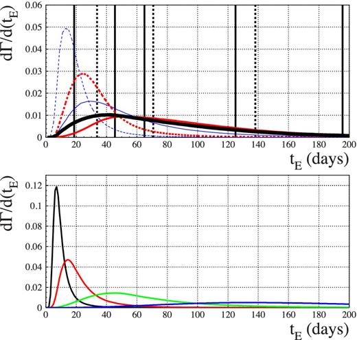
Normalized differential rate distribution, dΓ/dtE, corrected for the detection efficiency. Top panel: the expected distribution, each separately normalized, for the different self-lensing populations considered. Dashed and solid line are for the brown dwarf and star lenses, thin and thick lines for MW disc and SMC lenses. The thicker solid line is for the resulting overall self-lensing distribution. The dotted vertical lines indicate the 16 per cent, median and 84 per cent values of this distribution. The solid vertical lines indicate the values for the observed events, Table 1. Bottom panel: the expected distribution for MW MACHO lenses varying the MACHO mass. Moving from left to right as for the modal value: 0.01, 0.1, 0.5 and 1 M⊙.
In Table 4, we report the total number of expected events for the three experiment considered, EROS-2, OGLE-II and OGLE-III, for the self-lensing population considered, SMC self-lensing and MW disc lenses, for both the stellar and brown dwarf contribution, for the All and Bright sample, whenever the case. The inspection of this table suggests a few comments. As for the relative weight of the different experiment, for the All sample of sources, the OGLE-III expected signal is about three times larger than that of OGLE-II. The EROS-2 signal sums up to about half of that of the Bright sample of OGLE-III. The MW disc signal is overall rather small compared to the SMC self-lensing one. The different relative weight for OGLE-II and OGLE-III (about 7 per cent against 12 per cent) can be traced back mainly to the different extent of the monitored fields. The somewhat larger fraction for EROS-2, 17 per cent, can be understood on the basis of the larger efficiency for smaller values of the Einstein time. Overall, this makes EROS-2 quite relevant as compared to OGLE-III. Finally, although small, the expected SMC brown dwarf signal turns out to be about as large of the stellar MW disc one. Here again the relative increase for EROS-2 can be traced back to the different shape of the efficiency curve. Overall, the MW disc signal represents 10–16 per cent of the overall self-lensing signal. The enhancement of this ratio when considering the expected number as compared to the optical depth analysis is understood, given that Γ ∝ τ/tE, on the basis of the expected shorter duration of MW disc events.
Microlensing rate analysis: expected number of events for the self-lensing populations (BD stands for brown dwarfs) for each of the three experiment analysed.
| Lenses | OGLE-II | OGLE-III | EROS-2 | |
|---|---|---|---|---|
| All | All | Bright | Bright | |
| SMC | 0.36 | 1.25 | 0.71 | 0.33 |
| SMC DB | 0.036 | 0.13 | 0.079 | 0.045 |
| MW disc | 0.045 | 0.22 | 0.13 | 0.077 |
| MW disc BD | 0.0035 | 0.020 | 0.014 | 0.0093 |
| 0.44 | 1.62 | 0.93 | 0.46 | |
| Lenses | OGLE-II | OGLE-III | EROS-2 | |
|---|---|---|---|---|
| All | All | Bright | Bright | |
| SMC | 0.36 | 1.25 | 0.71 | 0.33 |
| SMC DB | 0.036 | 0.13 | 0.079 | 0.045 |
| MW disc | 0.045 | 0.22 | 0.13 | 0.077 |
| MW disc BD | 0.0035 | 0.020 | 0.014 | 0.0093 |
| 0.44 | 1.62 | 0.93 | 0.46 | |
The Palanque-Delabrouille et al. (1998) model strongly enhances the SMC self-lensing expected signal, resulting in about twice as much expected events. Coherently with the optical depth analysis these are found to be, however, much more strongly peaked in the innermost SMC region (for OGLE-III, for instance, we find that 60 per cent of the events should be expected in the innermost bin, defined as in the previous optical depth analysis, against 40 per cent for our fiducial model). In particular, the expected number of self-lensing events is 1.0 (OGLE-II), 3.1 and 1.8 (OGLE-III, All and Bright sample, respectively) and 0.8 (EROS-2). The major enhancement (about 2.5 times as much) is found, as expected, for the more centrally clustered OGLE-II fields of view.
The number of expected dark matter events, as a function of the MACHO mass for a full MACHO halo, is shown in Fig. 5. The expected increase in the number for smaller values of the MACHO mass is increasingly compensated by the corresponding decrease in the detection efficiency for small values of the event duration. In particular, coherently with the relative difference in their detection efficiency functions |${\cal E}(t_{\mathrm{E}})$|, the expected EROS-2 signal overtakes the OGLE-III one for values below 5 × 10⁻³ M⊙. Overall, the expected signal rapidly drops to zero below 10−3–10−4 M⊙ and, at the opposite end, above 1–10 M⊙. The expected peak values in the number of events is for a MACHO population in the mass range 10−2–10−1 M⊙.
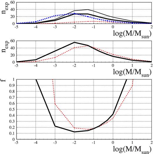
Top and middle panel: number of expected MW MACHO lenses events as a function of the MACHO mass for a full MACHO halo. Top panel: we report separately the results for OGLE-II (All sample), OGLE-III (All and Bright samples) and EROS-2 (dashed, thin solid, thick solid and dot–dashed lines, respectively). Middle panel: we report separately the results for the All sample (OGLE-II and OGLE-III, dashed line) and the Bright sample (OGLE-III and EROS-2, solid line). Bottom panel: 95 per cent CL upper limit for the halo mass fraction in form of MACHOs based on the Poisson statistics of the number of events (see the text for details). Solid and dashed curves as in the middle panel.
Overall, the relative ratios of the expected number of events from OGLE-II, OGLE-III (All and Bright sample) and EROS-2 are well understood starting from equation (9) and the specifications of the different set-up, in particular the value of the exposure, E, and the efficiency curve |${\cal E}(t_\mathrm{E})$|. OGLE-II enjoys a large exposure, EOGLE-II = 5.1 × 10⁹; however, it suffers from a quite small efficiency, below 10 per cent for tE < 10 d and rising at most up to about 16 per cent. For OGLE-III it results EOGLE-III = 1.7 × 10¹⁰ for the All sample and 4.9 × 10⁹ for the Bright sample for which, on the other hand, the efficiency is up to about twice as large than for the All sample. In particular, |${\cal E}(t_\mathrm{E})\sim 20$| per cent (10 per cent) for tE = 10 d, ∼30 per cent (13 per cent) at 20 d with top values about 50 per cent (25 per cent) in the range ∼ 120-300 d, for the Bright (All) sample, respectively. Finally, EROS-2 is characterized by a long duration but a relatively small number of monitored sources so that EEROS-2 = 2.3 × 10⁹, half as small |$E_\mathrm{OGLE-III}$| Bright sample. The strength of EROS-2 is however the efficiency reaching 30 per cent already at tE ∼ 10 d and remaining stable above 40 per cent in the range |$t_\mathrm{E}\sim 20{\rm -}140\,\mathrm{d}$|. On this basis we can understand, for instance, the large number of EROS-2 expected MACHO lensing events, in particular for low-mass values (10− 3-5 × 10− 2 M⊙), as compared to OGLE-II whereas the expected self-lensing signal, for EROS-2 and OGLE-II, turns out to be completely equivalent in terms of the number of expected events.
In the bottom panel of Fig. 5, we report the 95 per cent CL upper limit for the halo mass fraction in form of MACHOs, f, based on the Poisson statistics of the expected versus the observed number of events. In particular, we make use of the confidence level statistics for a Poisson distribution with a background, also following a Poisson distribution, whose mean value is supposed to be exactly known and which is given in our case by the expected self-lensing signal, following the recipe of Feldman & Cousins (1998). This gives us, in particular, the upper limit, fixed the confidence level, for the signal (the MACHO lensing number of events). We consider separately the full set of the All sample of sources (OGLE-II and OGLE-III) and the Bright one (OGLE-III and EROS-2). For the All (Bright) sample with nobs = 4 (3) reported candidate events and a background signal of nexp, SL = 2.06 (1.39) the 95 per cent CL upper limit turns out to be of 7.70 (6.86) events. The lowest upper limit (here and in the following at 95 per cent CL) for the Bright (All) sample is for 10−2 (5 × 10⁻²) M⊙ at f = 12 per cent (17 per cent), with f = 32 per cent (28 per cent) for 0.5 M⊙, respectively. The profile of the upper limit for the All and Bright sample follow, reversed, that of the expected number of MACHO lensing events modulated by the expected background signal values. In particular, when joining OGLE-II and OGLE-III for the All sample and OGLE-III and EROS-2 for the Bright sample, following the already remarked enhanced efficiency of EROS-2 to short duration (low-mass) events, the resulting constraints for f are stronger (also in an absolute sense) for the Bright sample for small mass values (here roughly below 0.1 M⊙), respectively, stronger for the All sample above this threshold.
In their analyses, the OGLE Collaboration, roughly based on the expected optical depth but lacking an explicit evaluation of the expected number of event for the self-lensing signal, and also following Moniez (2010), assumes that the background (self-lensing) expected value is equal to the number of observed events. In this case, four (three) for the All (Bright) sample, against our values, 2.1 (1.4), respectively. Under this assumption the upper limits for the signal, and therefore those on f, are accordingly smaller, in this case 5.76 (5.25), respectively (which makes, in relative terms, a rather significant change). For reference, we mention the values of these same upper limits assuming, instead, that the expected background is zero (namely assuming that there is no expected self-lensing signal), 9.76 and 8.25 for the All and Bright samples, respectively.
Starting from the larger values of expected self-lensing events with the Palanque-Delabrouille et al. (1998) model, 4.17 (2.59) for the All (Bright) sample, we would get to considerably smaller upper limit for the Poisson statistics with a background, 5.60 and 5.66 for the All and Bright sample, respectively (here the statistics makes the first value smaller, which is opposite to the result we obtain with our fiducial model). This then gives rise (the expected number of MACHO lensing events does not change) to stronger constraints for f (always at 95 per cent CL): in the range 12–16 per cent for 10− 2-0.2 M⊙ and 20 per cent at 0.5 M⊙ for the All sample and down to 10 per cent and below 20 per cent in the range 10− 3-0.2 M⊙ and 26 per cent at 0.5 M⊙ for the Bright sample.
4.4 The nature of the observed events
What is the nature of the observed lensing systems?, or, to rephrase it, is there any evidence for a signal from non-self-lensing population, namely, from MACHOs? We now attempt to address this issue starting from the results presented in the previous section, and in particular moving beyond the simple statistics based on the event number presented in the last section (Fig. 5).
4.4.1 The number of the events and their spatial distribution
OGLE-II reported one candidate event (All sample), for which we evaluate 0.44 expected self-lensing events. OGLE-III reported three (two) candidate events from the All (Bright) sample, with our evaluation of an expected self-lensing signal of 1.62 (0.93) events, respectively. Finally, EROS-2 reported one event out of a selected Bright subsample of sources, for which we evaluate an expected self-lensing signal of 0.46 events. Based on the underlying Poisson nature of the statistics of the detected events, the observed signal, according to the number of events, can be therefore fully explained by the expected self-lensing signal, according to our model most of it coming from faint SMC stars. As remarked, assuming an SMC model in agreement with that in Palanque-Delabrouille et al. (1998), for the same overall mass of the SMC luminous population, the number of expected self-lensing events is about twice as large than what we obtain with our fiducial model. This model, leaving aside the discussed issue of the spatial distribution of the events, would then lead to an even stronger confidence on the reliability of this outcome.
Although the statistics of events is not large, we may try to move beyond this considerations by exploiting the additional characteristics of the observed signal. We have already discussed the spatial distribution within the framework of the optical depth analysis. In fact, we expect the increase of the SMC self-lensing optical depth moving towards the SMC centre to be reflected in a corresponding increase of the expected signal in terms of the number of events. If we bin the observed field of view as in Section 4.1, we indeed find such an increase. For the MW lens populations, on the other hand, the expected distribution in terms of number of events is found to be roughly flat. These results are not surprising as the bins are chosen to contain an equal number of sources and therefore the expected signal follow the underlying optical depth profiles. To gain some further insight, we may evaluate the fraction of expected SMC self-lensing events, for each experiment, lying outside the contour of equal expected number of sources fixed by the position of the reported events. It results: 34, 28 and 38 per cent for EROS-2, OGLE-II and OGLE-III, respectively. For OGLE-III, the reported value is derived for the outermost event, and in this case we may also evaluate the fraction of expected events lying within the contour of the inner reported event, which turns out to be of 47 per cent (the corresponding fractions of source stars in these four cases are, respectively, 44, 33, 58 and 29 per cent). Assuming the Palanque-Delabrouille et al. (1998) model, we find again that the signatures of a much stronger gradient moving towards the SMC centre, namely the fraction, are significantly smaller (and larger for the last considered case). About 15 per cent of the events, for EROS-2, OGLE-II and OGLE-III, are expected out of the contour of equal number of sources fixed by the position of the outermost reported event (for a fraction of source stars equal to 38, 36 and 50 per cent, respectively) and, for OGLE-III, 72 per cent of the events are expected (with 35 per cent of the source stars) within the contour of the innermost reported event.
4.4.2 The duration distribution
Besides their position, the events are characterized by the duration. This is a useful statistics to our purposes as the duration distribution is independent from the expected event number. As a test case against the distribution of the observed durations, we consider the expected distribution for self-lensing events, SMC self-lensing and MW disc lenses, both stars and brown dwarf (Fig. 4). As a result, we find that the duration of two out of five events falls outside the 16–84 per cent range of probability for self-lensing lenses. More specifically, there is only about 5 per cent probability to get a self-lensing event duration shorter (longer) than that of OGLE-SMC-04 (OGLE-SMC-02). As apparent also from Fig. 4, short events are more likely for brown dwarf lenses, which represent, however, only about 10 per cent of the overall expected signal (Table 4). On the other hand, very long duration events look difficult to be explained (the case of OGLE-SMC-02, for which additional information is available to characterize the event, is further discussed below). To further quantify these statements, we may attempt to compare statistically the observed and the expected distributions. To this purpose, we consider the smaller but homogeneous set of the three All sample OGLE-III microlensing candidates, which span, incidentally, the full range of observed durations, tE = (18.6, 45.5, 195.6) d. To compare the observed and expected self-lensing duration distribution, first we make use of the Kolmogorov–Smirnov test which allows one to evaluate the probability of accepting the null hypothesis that the two distributions are indeed equal. This is known, however, to be specifically sensitive to compare the median values of the distributions, and in fact we find a rather large probability, 62 per cent. A similar statistics, built to be more sensitive to the outliers, is that of Anderson–Darling (Press et al. 1992) for which indeed the probability, which we evaluate through a simulation, drops to 32 per cent.
A final remark, quite apparent at glance from Fig. 4, is that, if not completely by self-lensing events, the very large spread of the observed durations distribution makes unlikely the possibility of explaining all the events by a single mass MACHO population (if any MACHOs).
4.4.3 The likelihood analysis
The likelihood analysis allows us to further address the issue of the nature of the events and in particular to quantify the limits for the halo mass fraction in form of compact halo objects, f. To this purpose, we proceed as detailed in Appendix A, taking, for reference, the expression of the likelihood in terms of the differential rate with respect to the event duration. This leads to include within the analysis both the line-of-sight position and the duration of the observed events. Fixing the MACHO mass as a parameter, given the likelihood, we may build the probability distribution for f, P(f), by Bayesian inversion assuming a constant prior different from zero in the interval (0, 1).
In Fig. 6, we show the results of the likelihood analysis, in particular we report the 95 per cent CL upper limit for f as a function of the MACHO mass. The curve shape reflects in part that of the expected number of MACHO events reported in Fig. 5, weighted, however, by the number and the specific characteristics of the observed events. Here, we consider separately the two cases of the four reported candidates from the All sample (OGLE-II and OGLE-III), and the three reported candidates from the Bright sample (OGLE-III and EROS-2), top and bottom panel in Fig. 6, respectively. For the All sample, we find the lowest constraint for f in the mass range 10− 2-10− 1 M⊙, with f ≤ 11–13 per cent. The upper limit then reduces to 30 per cent at 1 M⊙, at the same level than that at 10−3 M⊙. Whereas this second result is driven by the small number of expected MACHO lensing events there, the increase of the upper limit for f in the 10− 1-1 M⊙ range is rather driven by the characteristics of the events. The overall shape behaviour of the f upper limit is similar moving to the Bright sample. Here, however, thanks to the enhanced EROS-2 sensitivity to short duration events, we can put an f ∼ 10 per cent upper limit constraint over the range 10−3–10−1 M⊙, with the lowest value at f ∼ 7 per cent for 10−2 M⊙. The increase in the upper limit above 10−1 M⊙ is somewhat faster in this case, with f < 35 per cent at 1 M⊙. These behaviours, for the All and Bright sample, can also be more specifically explained on the basis of the event characteristics. In particular, the very short tE = 18.60 d OGLE-SMC-04 event, both in the All and in the Bright sample, somehow drives the results for low-mass values, up to about 10−1 M⊙, while the two long events, OGLE-SMC-02 and EROS2-SMC-1, both for the Bright sample, become relevant for large mass values (this is made apparent in particular by the, relatively, stronger constraint on f for 10 M⊙ in the All with respect to the Bright sample, where in the second case two out of three events are very long duration ones).
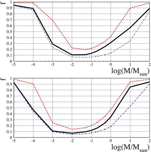
Likelihood analysis: 95 per cent CL upper limit for the mass halo fraction in the form of MACHO, f, as a function of the MACHO mass (in solar mass units) for All (OGLE-II and OGLE-III, top panel) and Bright (OGLE-III and EROS-2) sample of sources, solid lines. The dashed (dot–dashed) lines indicate the results we obtain under the hypothesis that the observed event are due to MACHO lensing (self-lensing), respectively.
A better understanding of the likelihood analysis results comes from the inspection of the dashed and dot–dashed upper limits in Fig. 6, where we report the results of the likelihood analysis under the assumption that the events are due to MACHO lensing (self-lensing), respectively (we remark that these results are based on the MACHO lensing signal only, namely the expected self-lensing rate does not enter the likelihood function). Both for the All and the Bright sample of sources, assuming that the events are self-lensing, the differences in the upper limit for f, comparing with the solid line where no hypotheses are done on the lens nature, are small up to about 10−2 M⊙ and then start increasing up to a rather large size. This somehow measures the extent to which, within the likelihood analysis, the events are weighted as self-lensing compared to MACHO lensing. In particular, this confirms that the MACHO lensing signal is strongly suppressed especially for low-mass values. The rather large difference in the two curves (solid and dot–dashed) for 10 M⊙ can also be understood on this basis recalling the very long durations events present in the All and Bright sample of sources. The dashed curve built assuming the events are MACHO, on the other hand, can be looked at as giving the more conservative upper limit for f, regardless of the characteristics of the events (just as the dot–dashed discussed above gives the less conservative one which can be obtained based on the available data). For the All sample, this is at about 20 per cent level in the range 10−2–10−1 M⊙, reducing to 40 per cent for 1 M⊙, whereas for the Bright sample the limit is up to about, in absolute sense, 6 per cent smaller in the lower range and, as before, significantly smaller at 10−3 M⊙ and, on the other hand, somewhat larger for 1 M⊙. Overall, the difference between the two curves (dashed and solid) is about constant at 10 per cent (in absolute sense) for the Bright sample all the way from MACHO mass above 10−3 M⊙. For the All sample, the difference is also of about 10 per cent but only within the range 10− 2-1 M⊙. Below and above these values, at 10−3 and 10 M⊙, the shape of the dashed curve then reflects the drop in the expected number of MACHO lensing events. The numerical detail of these results, also distinguishing each experimental set-up, is reported in Table 5.
Likelihood analysis: 95 per cent CL upper limit for f, the halo mass fraction in form of MACHOs for the All and the Bright sample. We report the results for the All sample for OGLE-II (1), OGLE-III (2) and OGLE-II plus OGLE-III (3–6); for the Bright sample for EROS-2 (1), OGLE-III (2) and EROS-2 plus OGLE-III (3–6). In columns (1–3), the likelihood is expressed in terms of the differential rate with respect to the event duration; in column (4) the likelihood is evaluated taking into account the number of expected events (Appendix 1); in column (5), (6) the upper limit on f is evaluated under the hypothesis that the observed events are (not) MACHOs.
| Mass | (1) | (2) | (3) | (4) | (5) | (6) |
|---|---|---|---|---|---|---|
| All sample | ||||||
| 10−3 M⊙ | 0.904 | 0.326 | 0.290 | 0.516 | 0.691 | 0.228 |
| 10−2 M⊙ | 0.665 | 0.120 | 0.107 | 0.167 | 0.224 | 0.073 |
| 0.1 M⊙ | 0.579 | 0.152 | 0.135 | 0.167 | 0.218 | 0.071 |
| 0.5 M⊙ | 0.789 | 0.261 | 0.247 | 0.255 | 0.333 | 0.109 |
| 1 M⊙ | 0.861 | 0.325 | 0.315 | 0.321 | 0.420 | 0.137 |
| 10 M⊙ | 0.928 | 0.615 | 0.567 | 0.755 | 0.896 | 0.345 |
| Bright sample | ||||||
| 10−3 M⊙ | 0.133 | 0.437 | 0.109 | 0.186 | 0.247 | 0.095 |
| 10−2 M⊙ | 0.105 | 0.160 | 0.072 | 0.111 | 0.139 | 0.053 |
| 0.1 M⊙ | 0.204 | 0.202 | 0.120 | 0.162 | 0.200 | 0.076 |
| 0.5 M⊙ | 0.468 | 0.366 | 0.245 | 0.290 | 0.356 | 0.138 |
| 1 M⊙ | 0.670 | 0.478 | 0.348 | 0.386 | 0.474 | 0.182 |
| 10 M⊙ | 0.944 | 0.859 | 0.851 | 0.873 | 0.938 | 0.526 |
We can compare the upper limits on f obtained within the likelihood analysis to those derived from the Poisson upper limits discussed in Section 4.3 and Fig. 5. Overall, they appear, quite significantly at least in a relative sense, larger. The driving motivation is the characterization as indistinguishable of the ‘signal’ with respect to the underlying ‘background’ one assumes to evaluate the upper limits, for the signal, for the Poisson distribution with a background (Feldman & Cousins 1998). The degeneracy in the lensing parameter space justify to some extent this characterization; however, the likelihood analysis allows one to take advantage of the specific characteristics of the observed events. It is also interesting to note that, within the scheme of the Feldman & Cousins (1998) statistics, assuming the mean expected background to be equal to the observed signal, one would get to about equal (and for some values of the MACHO mass, even tighter) constraints for f.
The results discussed above on the likelihood are obtained with our fiducial model. We may wonder what happens when using the Palanque-Delabrouille et al. (1998) model for which we expect about twice as much self-lensing events. As a result, we find that the upper limit we obtain in this case are indeed somewhat smaller, but the difference turns out never to exceed, in absolute sense, 3–4 per cent, namely, the two results are about equal. The underlying reason can be traced back in the spatial distribution of the observed events as compared to the expected signal which is, for the SMC self-lensing component, extremely more clustered around the SMC centre in the Palanque-Delabrouille et al. (1998) model. From a methodological point of view, this outcome clearly highlights the extent to which it is relevant to include within the analysis all the information available to draw meaningful conclusions on the MACHO lensing as compared to the self-lensing one, which is specifically what is made possible by the likelihood analysis.
To conclude on the likelihood analysis, we may address the question of whether the result we obtain is biased by our choice of expressing the likelihood in terms of the differential rate rather than considering the number of expected events (Appendix A). In this second case, corresponding to the line of sight of the observed events, the MACHO lensing and the self-lensing signals are compared based on the number of expected events only (in particular with no reference, therefore, to the observed event duration). As a result, Table 5, the upper limit in this case turns out to be larger, and this can be understood on the basis that in most cases the observed durations are in agreement with the self-lensing expected ones and, if not, as for the very long duration events, the expected MACHO lensing signal is however quite small: overall this attributes to the self-lensing rate more weight with respect to the MACHO lensing one than in the case where only the expected number (along a specific line of sight) is considered. The overall change, however, turns out to be not too large, in an absolute if not relative sense, compared to the results reported in Fig. 6. In particular, the difference is about 5 per cent and up to 10 per cent in the mass range 10− 2-1 M⊙ and 10− 3-10 M⊙ for the All and the Bright sample, respectively, with the difference which tends to be larger for small mass values. The larger difference, about 20 per cent, we find for the All sample at 10−3 and 10 M⊙ should, as above, be traced back in the drop of the expected MACHO lensing signal to a level almost compatible with the self-lensing one.
4.4.4 The projected velocity: the case of OGLE-SMC-02
Although the likelihood analysis is driven by the characteristics of the observed events, it remains a statistical approach on a full set of events. Further insight into the nature of the lenses can be gained for those events for which additional information is available. Within the present set of events, this is specifically the case for the long duration (tE = 195.6 d) OGLE-SMC-02 candidate event. As discussed in Section 3, Dong et al. (2007) did conclude strongly in favour of the MW MACHO nature of this event. In general, the analysis of the MACHO hypothesis suffers from the degeneracy within the lensing parameter space of the unknown lens mass. As apparent also from inspection of the differential rate distribution, Table 3 and Fig. 4, a long-duration event as OGLE-SMC-02 might indeed be explained by a heavy (∼(1–10) M⊙) MACHO, possibly a black hole. This conclusion is however dependent on an hypothesis on the lens mass. Within their analysis, Dong et al. (2007) could get rid of this limitation. In particular, they were able to provide an estimate of the projected velocity (Gould 1994) |$\tilde{v}=v/(1-D_{\rm l}/D_{\rm s})$|, a quantity which is only weakly dependent on the lens mass (and altogether independent if assuming a delta mass function), with |$\tilde{v}_\mathrm{obs}\sim 230\,\mathrm{km s}^{-1}$|. We have evaluated the expected differential distribution for |$\mathrm{d}\Gamma /\mathrm{d}\tilde{v}$| given our fiducial model for the SMC self-lensing, MW disc and MW MACHO populations (from equation (7), we evaluate |$\mathrm{d}\Gamma /\mathrm{d}\tilde{v} = \mathrm{d}\Gamma /\mathrm{d}v \times (1-D_{\rm l}/D_{\rm s})$|). The result of this analysis is reported in Fig. 7. At glance, the estimated observed value, |$\tilde{v}_\mathrm{obs}$|, is in good agreement with the MW MACHO lensing population projected velocity distribution and at odds with that of the self-lensing populations. In particular, the probability of getting a smaller (larger) value than |$\tilde{v}_\mathrm{obs}$| is below 1 per cent for SMC star (MW disc) lenses.
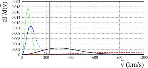
Normalized differential rate |$\mathrm{d}\Gamma /\mathrm{d}\tilde{v}$|, where |$\tilde{v}=v/(1-D_{\rm l}/D_{\rm s})$| is the projected velocity, along the line of sight of OGLE-SMC-02 microlensing candidate event (tE = 195.6 d). In particular, we show the result for different lens populations: MW thin disc, MW thick disc, SMC self-lensing and MW MACHO lensing (dotted, dash–dotted, dashed, solid lines, respectively). The vertical solid line represents the estimated observed value.
Looking back to the initial issue, the nature of the observed events, we have therefore shown that, although the bare number of observed versus expected events may suggest that all of them may be attributed to self-lensing populations, a more thorough analysis, considering the full set of available event characteristics, leads us at very least to soften this conclusion. On the other hand, if any, the extent of the MACHO population compatible with the available data would clearly remain very small.
5 COMPARISON TO PREVIOUS ANALYSES
It is also interesting to compare the line of sight towards the SMC to that towards the LMC. Here again we take advantage of the OGLE-III analysis (Wyrzykowski et al. 2011a), which we also have discussed in Calchi Novati & Mancini (2011), to carry out an homogeneous comparison. As for the MACHO lensing signal, it is useful again to start from equation (10). The LMC counts almost four times more numerous source stars, which more than compensates the decrease in the ratio τ/〈tE〉 discussed above. Based on these terms, fixed Tobs, one should expect almost three times more MACHO lensing events towards the LMC than towards the SMC. The efficiency however, at least following the OGLE-III analysis, tends to reduce this difference, especially for the Bright sample (indeed, the efficiency towards the LMC greatly varies from field to field according to the relative crowding, whereas towards the less crowded SMC fields, it results roughly constant across the monitored fields of view and, especially for the Bright sample, relatively larger). As for self-lensing, lensing by SMC stars is strongly enhanced by the SMC morphology compared to LMC self-lensing; on the other hand the overall MW disc lensing signal is relatively much more important for the LMC because of the much larger extension of the monitored field of view. Overall, the expected self-lensing signal towards the LMC turns out to be about twice as large as that towards the SMC. Face to these changes in the expected signal, the observed rate, for the OGLE-III analysis, turns out, with the caveat of the small statistics, to be fully compatible towards the two lines of sight: for the All sample, two (three) candidate events are reported towards the LMC (SMC). These effects therefore combine so that the constraints on f from the LMC turns out to be tighter.
6 CONCLUSIONS
In this paper, we have discussed the results of the microlensing campaigns carried out towards the SMC by the EROS (Tisserand et al. 2007) and the OGLE collaborations (Wyrzykowski et al. 2010, 2011b). In particular, we have addressed the issue of the nature of the lens of the observed events, either to be attributed to ‘self-lensing’, where the lens belong to some luminous component (either of the SMC or of the MW disc) as opposed to MACHO lensing from the putative population of dark matter compact halo objects of the MW. To this purpose, we have carried out analyses of the microlensing optical depth and of the expected signal based on the evaluation of the microlensing rate.
Overall, five microlensing candidates have been reported (one each by EROS-2 and OGLE-II and three by OGLE-III). Whereas in terms of number of events, this may be fully explained by the expected self-lensing signal (out of which about 90 per cent is expected from SMC self-lensing), the analyses based on the event characteristics, line-of-sight position and duration, and for one event on the evaluation of the projected velocity, rather suggest that not all the events may be attributed to this lens population. In particular, 2.1 (1.4) self-lensing events are expected, to be compared to 4 (3) observed events, depending on the sample of sources considered. Two events (both reported by OGLE-III) have durations lying outside the 95 per cent limits of the expected self-lensing signal (one shorter, one longer). The long-duration event is the same for which the projected velocity analysis, which strongly favour a non-self-lensing nature of the lens, has been carried out (Dong et al. 2007). Additionally, we have discussed the spatial distribution of the observed events as compared to the profile of the SMC self-lensing optical depth. Finally, both the event line-of-sight position and duration enter the likelihood analysis. Taking into account the expected signal of the self-lensing and MACHO lensing populations, this allows us to quantify the resulting upper limit on the halo mass fraction in form of MACHOs, f. In particular, it results that the upper limit at 95 per cent CL is lowest, about 10 per cent, at 10−2 M⊙, and then reduces to above 20 per cent for 0.5 M⊙ MACHOs. Overall, these limits are somewhat less tight than those obtained by analogous analyses carried out towards the LMC (Tisserand et al. 2007; Wyrzykowski et al. 2011a) where, also compared to a somewhat larger expected signal in terms of MACHO lensing events, the number of observed events is not correspondingly larger. Larger set of events, hopefully available in the next future thanks to the ongoing OGLE-IV and MOA-II campaigns should provide further insight in this problem.
The expected SMC self-lensing signal is driven by the underlying model of the SMC luminous components for which, in this work, we have taken advantage of several recent analyses (Bekki & Chiba 2009; Haschke et al. 2012; Subramanian & Subramaniam 2012, and references therein), which however still do not provide a full coherent picture of its formation history, dynamic and morphology. Among the more relevant quantities for microlensing purposes, the value for the line-of-sight depth seem quite well established. There remain however still open questions as the overall luminous SMC mass and the exact balance between the old and the YS populations. A correct model for the SMC luminous remains a key issue for the understanding of the microlensing signal. Indeed, a larger set of events would make even more important a detailed knowledge of the SMC morphology, providing a further relevant tool of analysis to address the issue of the lens nature.
We thank the referee for valuable comments and remarks. We thank Łukas Wyrzykowski for several fruitful discussions on the OGLE analysis. We thank Kenji Bekki for discussions on the SMC model. SCN and GS acknowledge support by the Swiss National Science Foundation during part of this work. PJ and SM acknowledge support by the Swiss National Science Foundation.
There is a caveat concerning the total mass and the corresponding normalization of this model. In fact, although Palanque-Delabrouille et al. (1998) report a stellar mass of ∼1 × 10⁹ M⊙, which corresponds to our chosen normalization for the SMC luminous mass within 5 kpc, we have to introduce a multiplicative factor 1.6, which we use, in the density normalization, with respect to the values reported in Palanque-Delabrouille et al. (1998), to match the overall mass of our model within the tidal radius.
The time-scale of a microlensing event is the Einstein time, tE = RE/v, where v is the (transverse component of the) lens velocity with respect to the microlensing tube.
For cross-check, the evaluation of the optical depth profiles has been carried out independently by two of us.
REFERENCES
APPENDIX A: THE LIKELIHOOD ANALYSIS
The terms xi, being related to the expected number of events per bin, are proportional to the microlensing rate. As a possible approach, one can introduce a binning in the duration, ΔtE, and then reduce to equation (A1) by the limit ΔtE → 0. In this case x = dΓ/dtE, evaluated at the value of the observed durations, tE, obs. This is the likelihood expression used, for instance, in the analyses of the MACHO group [Alcock et al. (2000) and references therein]. Alternatively, one can directly consider x as the number of expected events per bin evaluated according to equation (9). This gives the likelihood analysis used, for instance, within the analysis of M31 pixel lensing results of the POINT-AGAPE Collaboration (Calchi Novati et al. 2005). Whatever the choice, the underlying structure of equation (A1) drives the resulting limit on f.
The rate, and therefore the expected number of events, can be looked at as the sum of two terms: the self-lensing contribution plus the MACHO lensing contribution modulated the multiplicative factor f. As a first remark, we note that in the exponential term, exp (−Nexp), the number of expected self-lensing events drops out as a constant. In particular, this implies that for no observed events, either assuming that the observed events are due to self-lensing, the resulting limits on f are independent from the expected self-lensing signal and are driven by the expected number of MACHO lensing events only. In the more general case of Nobs > 0, the exponential decrease of f is modulated by Nobs factors of the kind a + fb, where a and b are constants with respect to f and linked to the expected self-lensing and MACHO lensing signal, respectively. To the purpose of the evaluation of the probability distribution for f, P(f), only the ratio b/a matters so that whatever factor coming in front of both of them drops out in the normalization of P(f). In particular, for the choice mentioned above, x = dΓ/dtE, when calculating the differential rate at the observed duration value, the efficiency term |${\cal {E}}(t_\mathrm{E})$| does drop out (being usually given as a unique function for all the lens populations considered). On the other hand, when considering for x the number of expected events, the efficiency |${\cal {E}}(t_\mathrm{E})$| enters in an essential way, whereas the constants that drop out are the number of sources and the overall time span of the experiment, so that in particular one can consider, for instance, as the infinitesimal bin choice, the lines of sight corresponding to each observed event. It is also important to keep track that in these two cases one is in fact weighting the event characteristics in a different way. In the first case, both the event line-of-sight position and the duration enter the likelihood (with the relevant caveat that the duration is not modulated by the detection efficiency). In the second, the results are driven specifically by the expected number of events within the chosen bins, namely the line-of-sight position. The outcome is therefore expected to be more similar to the analysis carried out based on the number of events according to the Poisson distribution. This is not surprisingly as the underlying statistics is the same, with the important caveat, however, that within this likelihood-based analysis also the observed event spatial distribution is included within the analysis.
In the present analysis, we consider the joint results from more than one experiment. In this case, the probabilities, and therefore the different likelihood term, multiply. Each experiment is characterized by his own number of expected events and this fixes, through the exponential term in the likelihood, the relative weight of each of them. On the other hand, all the reported events, appearing in the product, enter the likelihood on the same footing.
