On the signature of z ∼ 0.6 superclusters and voids in the Integrated Sachs–Wolfe effect

Hernández-Monteagudo, Carlos; Smith, Robert E.

doi:10.1093/mnras/stt1322

Abstract

Through a large ensemble of Gaussian realizations and a suite of large-volume N-body simulations, we show that in a standard Λ cold dark matter (ΛCDM) scenario, supervoids and superclusters in the redshift range z ∈ [0.4, 0.7] should leave a small signature on the Integrated Sachs–Wolfe (ISW) effect of the order of ∼ 2 μK. We perform aperture photometry on Wilkinson Microwave Anisotropy Probe (WMAP) data, centred on such superstructures identified from SDSS luminous red Galaxies data, and find amplitudes at the level of 8–11 μK – thus, confirming the earlier work of Granett et al. If we focus on apertures of the size ∼3| $_{.}^{\circ}$|6, then our realizations indicate that ΛCDM is discrepant at the level of ∼4 σ. However, if we combine all aperture scales considered, ranging from 1°to 20°, then the discrepancy becomes ∼2 σ, and it further lowers to ∼0.6 σ if only 30 superstructures are considered in the analysis (being compatible with no ISW signatures at 1.3 σ in this case). Full-sky ISW maps generated from our N-body simulations show that this discrepancy cannot be alleviated by appealing to Rees–Sciama mechanisms, since their impact on the scales probed by our filters is negligible. We perform a series of tests on the WMAP data for systematics. We check for foreground contaminants and show that the signal does not display the correct dependence on the aperture size expected for a residual foreground tracing the density field. The signal also proves robust against rotation tests of the cosmic microwave background maps, and seems to be spatially associated with the angular positions of the supervoids and superclusters. We explore whether the signal can be explained by the presence of primordial non-Gaussianities of the local type. We show that for models with |${f_{\rm NL}^{\rm local}}=\pm 100$|⁠, whilst there is a change in the pattern of temperature anisotropies, all amplitude shifts are well below < 1 μK. If primordial non-Gaussianity were to explain the result, then |${f_{\rm NL}^{\rm local}}$| would need to be several times larger than currently permitted by WMAP constraints.

galaxies: clusters: general, cosmic background radiation, cosmology: observations, large-scale structure of Universe

1 INTRODUCTION

Over the last 15 years, evidence has been mounting from various cosmological probes to support the case for an accelerating universe. It can be argued that the first compelling evidence for this arose from the study of the light curves of distant Type Ia supernovae (Riess et al. 1998; Perlmutter et al. 1999). Currently, the strongest support for this picture comes from the combination of observations of the cosmic microwave background radiation (hereafter CMB), and from measurements of the clustering of galaxies. From the CMB side, the Wilkinson Microwave Anisotropy Probe (hereafter, WMAP) experiment (Spergel et al. 2003, 2007; Komatsu et al. 2011)¹ provided a precise measurement of the angular size of the sound horizon at recombination, which supported the case for a spatially flat universe. On the clustering side, data from surveys like the two-degree Field Redshift Survey (Cole et al. 2005) and the Sloan Digital Sky Survey (hereafter SDSS) (Tegmark et al. 2006) required the density in matter to be sub-critical, hence leading to the inference that ∼70 per cent of the current energy density of the Universe is in a form of energy that behaves like a cosmological constant, and so acts as a repulsive gravitational force. The energy density driving the accelerated expansion is unknown and so has been dubbed Dark Energy (hereafter DE). Uncovering the true physical nature of the DE is one of the main targets for many ongoing and upcoming surveys of the Universe.

Standard linear cosmological theory states that if the Universe undergoes a late-time phase of accelerated expansion, then gravitational potential wells on very large scales ( ≳ 100 h^{− 1} Mpc) will decay. This evolution of the potential wells introduces a gravitational blueshift in the photons of the CMB that is known as the Integrated Sachs–Wolfe effect (ISW). This effect constitutes an alternative window to DE, and can be directly measured by cross-correlating CMB maps with a set of tracers for the density field, which sources the potentials (Crittenden & Turok 1996). As soon as the first data sets from WMAP were released, several works claimed detections of the ISW at various levels of significance (Fosalba, Gaztañaga & Castander 2003; Scranton et al. 2003; Afshordi, Loh & Strauss 2004; Boughn & Crittenden 2004; Fosalba & Gaztañaga 2004; Nolta et al. 2004; Padmanabhan et al. 2005; Cabré et al. 2006; Giannantonio et al. 2006; Vielva, Martínez-González & Tucci 2006; McEwen et al. 2007). Subsequent analysis has led some researchers to be more cautious about interpreting these early detections (Hernández-Monteagudo, Génova-Santos & Atrio-Barandela 2006; Rassat et al. 2007; Bielby et al. 2010; Francis & Peacock 2010; Hernández-Monteagudo 2010; López-Corredoira, Sylos Labini & Betancort-Rijo 2010). As emphasized by Hernández-Monteagudo (2008), the true ISW effect should only be detectable for deep galaxy surveys that cover a substantial fraction of the sky. However, an erroneous interpretation of ISW cross-correlation studies may be obtained from systematic errors, such as residual point source emission in CMB maps or presence of spurious galaxy auto-power on large angular scales (see also Hernández-Monteagudo 2010, for details on the WMAP–NVSS cross-correlation analysis.). In particular, the issue of excess power on large scales has been noted in several works (Ho et al. 2008; Hernández-Monteagudo 2010; Thomas, Abdalla & Lahav 2011; Giannantonio et al. 2012), but it is not yet fully accounted for.

Amongst the subsequent ISW cross-correlation studies in the literature, there is the particularly puzzling work of Granett, Neyrinck & Szapudi (2008, hereafter G08). Their analysis yielded one of the highest detection significances in the literature. G08 implemented the following novel approach: they produced a catalogue of superclusters and supervoids from SDSS data, and stacked WMAP-filtered data on the positions of these structures with apertures of the order of ∼4°. They obtained an ∼4σ ISW detection. Unlike previous works on the subject, the analysis focused on a particular sub-set of the available large-scale structure (hereafter LSS) data. Subsequent studies have investigated the origin of the signal and assessed its compatibility with the Λ cold dark matter (ΛCDM) scenario, (Pápai & Szapudi 2010; Pápai, Szapudi & Granett 2011; Nadathur, Hotchkiss & Sarkar 2012). While some works found the G08 results compatible, others found the measured amplitudes too high to be consistent (Granett, Neyrinck & Szapudi 2009; Inoue, Sakai & Tomita 2010; Inoue 2012; Nadathur et al. 2012; Flender, Hotchkiss & Nadathur 2013). Currently, the G08 results remain unexplained.

In this work, we shall attempt to shed new light on this problem. The paper breaks down as follows: In Section 2, we give a brief theoretical overview of the ISW effect, underlining the expectation for the ISW signal from a cross-correlation analysis of the data used in G08. In Section 3, we perform a cross-check of the G08 results. In Section 4, we test whether the G08 results are consistent with expectations for the ΛCDM model. This is achieved by using a large ensemble of Gaussian Monte Carlo realizations. We also generate full-sky non-linear ISW maps by ray-tracing through a suite of N-body simulations. In Section 5, we determine the level of significance at which the results disagree with the ΛCDM paradigm. We explore systematic errors in the foreground subtraction for WMAP. We also investigate whether the excess signal is consistent with primordial non-Gaussianities of the local type. Finally, in Section 6 we summarize our findings and conclude. While this paper was in the process of submission, a parallel work on this subject from Flender et al. (2013) appeared in the internet. This work is reaching to similar conclusions to ours in some of the issues addressed in this work.

Unless stated otherwise, we employ a reference cosmological model consistent with WMAP7 (Komatsu et al. 2011): the energy-density parameters for baryons, CDM and cosmological constant are Ω_b = 0.0456, Ω_cdm = 0.227, Ω_Λ = 0.7274; the reduced Hubble rate is h = 0.704; the scalar spectral index is n_S = 0.963; the rms of relative matter fluctuations in spheres of 8 h⁻¹ Mpc radius is σ₈ = 0.809 and the optical depth to last scattering is τ = 0.087.

2 THEORETICAL PERSPECTIVE

2.1 The ISW effect

Observed CMB photons are imprinted with two sets of fluctuations: primary anisotropies, sourced by fluctuations at the last-scattering surface, and secondary anisotropies, induced as the photon propagates through the late-time clumpy Universe. The physics of the primary anisotropies is well understood (Dodelson 2003; Weinberg 2008). There are a number of physical mechanisms that give rise to the generation of secondary anisotropies (for a review see The Planck Collaboration 2006) and one of these is the redshifting of the photons as they pass through evolving gravitational potentials. The linear version of this effect is termed the ISW effect (Sachs & Wolfe 1967) and its non-linear counter-part is termed the Rees–Sciama effect (Rees & Sciama 1968).

The observed temperature fluctuation induced by gravitational redshifting may be written as (Sachs & Wolfe 1967)

\begin{equation} \frac{\Delta T({\hat{\boldsymbol n}})}{T_0} = -{2 \over c^2}\int _{t_{\rm ls}}^{t_{0}}\mathrm{d}t \,\dot{\Phi }({\hat{\boldsymbol n}},\chi ) \ , \end{equation}

(1)

where |${\hat{\boldsymbol n}}$| is a unit direction vector on the sphere, Φ is the dimensionless metric perturbation in the Newtonian gauge, which reduces to the usual gravitational potential on small scales, the ‘over dot’ denotes a partial derivative with respect to the coordinate time t from the FLRW metric, χ is the comoving radial geodesic distance |$\chi =\int c\text{d}t/a(t)$|⁠, and so may equivalently parametrize time. The symbols t₀ and t_ls denote the time at which the photons are received and emitted, i.e. the present time and last scattering. c is the speed of light and a(t) is the dimensionless scale factor.

On scales smaller than the horizon, relevant to our simulation boxes, the perturbed Einstein equations in Newtonian gauge lead to a perturbed Poisson equation. This enables us to relate potential and matter fluctuations (Dodelson 2003):

\begin{equation} \nabla ^2\Phi ({\boldsymbol x};t)=4\pi G\bar{\rho }(t)\delta ({\boldsymbol x};t) a^2\!(t) \,, \end{equation}

(2)

where |$\bar{\rho }(t)$| is the mean matter density in the Universe and the density fluctuation is defined |$\delta ({\boldsymbol x};t)\equiv [\rho ({\boldsymbol x},t)-\bar{\rho }(t)]/\bar{\rho }(t)$|⁠. This equation may most easily be solved in Fourier space:

\begin{equation} \Phi ({\boldsymbol k};t) = -4\pi G\bar{\rho }(t)a^2(t)\frac{\delta ({\boldsymbol k};t)}{k^2}\,. \end{equation}

(3)

Differentiation of the above expression gives

\begin{equation} \dot{\Phi }({\boldsymbol k};t) = \frac{3}{2}\Omega _{\rm m0} H_0^2 k^{-2} \left[ \frac{H(t)}{a(t)}\delta ({\boldsymbol k};t)-\frac{\dot{\delta }({\boldsymbol k};t)}{a(t)} \right] \,, \end{equation}

(4)

where we used the fact that |$[a^3(t)\bar{\rho }(t)]$| is a time-independent quantity in the matter-dominated epoch and Ω_m ≡ Ω_cdm + Ω_b. In the above, we also defined |$H(t)\equiv \dot{a}(t)/a(t)$| and |$\Omega _{\rm m}(t)\equiv \bar{\rho }(t)/\rho _{\rm crit}(t)$|⁠, with ρ_crit(t) = 3H²(t)/8πG. All quantities with a subscript 0 are to be evaluated at the present epoch. In the linear regime, density perturbations scale as |$\delta ({\boldsymbol k},a)=D(a)\delta ({\boldsymbol k},a_0)$|⁠. Inserting this relation into equation (4) gives

\begin{equation} \dot{\Phi }({\boldsymbol k};t) = \frac{3}{2}\Omega _{\rm m0} H_0^2 k^{-2} \frac{H(t)}{a(t)} \left[ 1 -\frac{d\log D}{d\log a}\right] \delta ({\boldsymbol k};a) \,. \end{equation}

(5)

In the matter-dominated phase, the Universe expands as in the Einstein–de Sitter case and consequently density perturbations scale as D(a) ∝ a. Thus, for most of the evolution of the late-time Universe the bracket, [1 − d log D/dlog a] is close to zero. In the ΛCDM model, it is only at relatively late times that this term is non-zero.

Alternatively, in the non-linear regime δ(k, a) ≠ D(a)δ(k, a₀) and this gives rise to additional sources for the heating and cooling of photons (Smith, Hernández-Monteagudo & Seljak 2009; Cai et al. 2009, 2010).

2.2 Expectations for cross-correlation analysis

The expected signal for the ISW-density tracer cross-correlation analysis has been described by several authors (Crittenden & Turok 1996; Hernández-Monteagudo 2008; Smith et al. 2009) and here we simply quote the main results. For a survey of galaxies (or more generically, objects that are biased density tracers) the ISW-density angular cross-power spectrum can be written:

\begin{eqnarray} C_{\ell }^{\rm g, ISW} & = & \left( \frac{2}{\pi }\right)\int _0^{\infty } \;k^2\mathrm{d}k\; P_{\rm m}(k) \; \nonumber \\ && \times \int _{0}^{\infty } \mathrm{d}\chi _1\; j_{\ell } (k\chi _1) \chi _1^2 W_{\rm g}(\chi _1)n_{\rm g}(\chi _1)b(\chi _1,k)D(\chi _1) \nonumber \\ && \times \int _{0}^{\infty } \mathrm{d}\chi _2\; j_{\ell } (k\chi _2) \frac{-3\Omega _{\rm m}H_0^2}{k^2} \;\frac{\mathrm{d}(D(\chi _2)/a(\chi _2))}{\mathrm{d}\chi _2} \,, \end{eqnarray}

(6)

where P_m(k) denotes the linear matter power spectrum at the present time, the super-script g refers to the objects (galaxies in most cases, but in ours it will refer to voids or superclusters) probing the gravitational potential wells. In the above n_g(χ) denotes the average comoving object number density; W_g(χ) denotes the instrumental window function providing the sensitivity of the instrument to the objects at distance χ; the j_ℓ(x) are the usual spherical Bessel functions of order l; and b(χ, k) denotes the bias of the tracer population with respect to the matter density field. This last factor may be both a function of time χ and scale k (Smith, Scoccimarro & Sheth 2007), but for simplicity we shall simply assume that the bias equals unity for the objects in our catalogue.

In this measurement, the primary CMB signal acts as noise. If we take this into account and also the variance due to the density field, then the |${\mathcal {S}}/{\mathcal {N}}$| with which we expect to detect the cross-correlation for a given multipole is (e.g. Crittenden & Turok 1996)

\begin{eqnarray} \left(\frac{\mathcal {S}}{\mathcal {N}} \right)^2_{\ell } & = & \frac{\left(C_{\ell }^{\rm g,ISW}\right)^2\times (2\ell +1)f_{\rm sky}}{C_{\ell }^{\rm CMB}\left(C_{\ell }^{\rm g} + 1/{\bar{n}}_{\rm g}\right)+\left(C_{\ell }^{\rm g,ISW}\right)^2} \,, \end{eqnarray}

(7)

where |$C_{\ell }^{\rm CMB}$| and |$C_{\ell }^{\rm g}$| represent the auto power spectra of the temperature fluctuations and the density tracers; |$\bar{n}_{\rm g}$| denotes the average angular object number density and hence the term |$1/{\bar{n}}_{\rm g}$| denotes the shot-noise. In our forecast, we shall neglect this term (hence the predicted significance will be slightly overoptimistic). The factor |$f_{\text{sky}}$| refers to the fraction of the sky jointly covered by both the CMB and the object surveys. The cumulative |${\mathcal {S}}/{\mathcal {N}}$| for all harmonics smaller than l can then be written:

\begin{equation} \frac{\mathcal {S}}{\mathcal {N}} (<\!\!\ell ) = \sqrt{\sum _{\ell ^{\prime }=2}^{\ell } \left( \frac{\mathcal {S}}{\mathcal {N}}\right)^2_{\ell ^{\prime }}}, \end{equation}

(8)

where the monopole and dipole have not been included.

2.3 Expectations for ISW from data used in Granett et al.

We now turn to the question of what |${\mathcal {S}}/{\mathcal {N}}$| should G08 have expected to find in their data. G08 used a sample of 1.1 million luminous red Galaxies (hereafter LRG) selected from the SDSS data release 6 (hereafter DR6) (Adelman-McCarthy et al. 2008). This sample covered roughly 7500 square degrees and spanned a redshift range of (0.4 < z < 0.75). From this sample, they identified regions as supervoids or superclusters using the algorithms ZOBOV and VOBOZ,² respectively, (Neyrinck, Gnedin & Hamilton 2005; Neyrinck 2008). The significance of these regions was chosen to be at least at the 2σ level relative to a Poisson sample of points. G08 selected the largest 50 superclusters and supervoids for their analysis. Their catalogue is publically available.³

In the left-hand panel of Fig. 1, the dot–dashed and dotted histograms denote the redshift distributions of supervoids and superclusters, respectively. The thick solid line represents an analytic fit that we have constructed, which attempts to be a compromise between the two. Our fitting function extends to slightly lower redshifts than the G08 catalogue, and this will translate into a slightly higher ISW prediction.

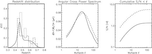
$Left-hand panel: redshift distribution of supervoids and superclusters for the catalogue provided by G08 from the SDSS DR6 data. The dotted histogram denotes supervoids and the dot–dashed histogram denotes superclusters. The solid line represents an analytic approximation, which is a compromise between both histograms. Middle panel: angular cross-power spectrum between ISW and the projected density. The solid line denotes the predictions for both supervoids and superclusters, modulo the bias being unity. The dashed curve represents what one would expect for QSO's in the NVSS survey. Right-hand panel: cumulative ${\mathcal {S}}/{\mathcal {N}}$ below a given multipole ℓ. The solid line denotes the prediction for matter within the redshift distribution sampled by the G08 catalogue. The dashed line presents the predictions for QSO's in NVSS.$

Figure 1.

Left-hand panel: redshift distribution of supervoids and superclusters for the catalogue provided by G08 from the SDSS DR6 data. The dotted histogram denotes supervoids and the dot–dashed histogram denotes superclusters. The solid line represents an analytic approximation, which is a compromise between both histograms. Middle panel: angular cross-power spectrum between ISW and the projected density. The solid line denotes the predictions for both supervoids and superclusters, modulo the bias being unity. The dashed curve represents what one would expect for QSO's in the NVSS survey. Right-hand panel: cumulative |${\mathcal {S}}/{\mathcal {N}}$| below a given multipole ℓ. The solid line denotes the prediction for matter within the redshift distribution sampled by the G08 catalogue. The dashed line presents the predictions for QSO's in NVSS.

Open in new tab Download slide

The middle panel of Fig. 1 presents the angular cross-power spectrum as predicted by linear theory for the void/supercluster catalogue (solid line). Recall that we are taking b = 1 for both voids and clusters. In reality, the void/cluster regions will be antibiased/biased and so the two signals will differ. However, since here we are more concerned with the |${\mathcal {S}/N}$| this simplification does not matter, especially since we are neglecting the effects of shot-noise on the cross-spectra. We also point out that our predictions for the ISW-induced cross-correlation signal of superclusters and supervoids in the SDSS sample are quite similar to the predictions for the cross-correlation of AGNs (z < 2) in the NVSS catalogue (after adopting the model of Ho et al. 2008, see the dashed line in the middle panel of Fig. 1).

The right-hand panel of Fig. 1 presents the predictions for the cumulative |${\mathcal {S}}/{\mathcal {N}}$| for the SDSS supercluster and supervoid analysis. These predictions (solid black line) show that, for a ΛCDM model, one should expect no more than ≃1.3σ significance. In contrast, the prediction for NVSS (dashed line) is close to ∼5.5 (obtained after also neglecting shot noise). This is not surprising, since the G08 supervoid and supercluster catalogue is relatively shallow, spanning the redshift range (0.4 < z < 0.7), and covers only a modest fraction of the sky (f_sky ≃ 0.18). The NVSS is instead significantly deeper and wider. We hence conclude that had G08 applied a standard ISW cross-correlation analysis to their data, then in the framework of the ΛCDM model, there would have been very little chance for detecting any genuine signal at high significance.

3 CROSS-CHECKING GRANETT ET AL.

3.1 CMB data

The WMAP experiment scanned the CMB sky from 2001 until 2010 in five different frequencies, ranging from 23 to 94 GHz. The angular resolution in each band improves with the frequency, but it remains better than one degree in all bands. The |${\mathcal {S}}/{\mathcal {N}}$| is greater than one for multipoles ℓ < 919 (Jarosik et al. 2011), and in particular, on the large scales of interest for ISW studies, the galactic and extragalactic foreground residuals are below the 15μK level outside the masked regions (Gold et al. 2011).

We concentrate our analysis on the foreground-cleaned maps corresponding to bands Q (41 GHz), V (61 GHz) and W (94 GHz), after applying the conservative foreground mask KQ75y7, which excludes ∼25 per cent of the sky. At the scales of interest, instrumental noise lies well below cosmic variance and foreground residuals, and hence will not be considered any further. The ISW is a thermal signal whose signature should not depend upon frequency and hence should remain constant in the three frequency channels. All of the WMAP data employed in this analysis were downloaded from the lambda site.⁴

3.2 Supercluster and supervoid data

For our tracers of the LSS, we use the same supercluster and supervoid catalogue as used by G08. As described earlier, the catalogue was constructed after applying the ZOBOV and VOBOZ algorithms to search for supervoids and superclusters in the LRG sample extracted from SDSS DR6, respectively. G08 used the 50 largest supervoids and superclusters. They claimed that this cut yielded the highest statistical significance, in that it minimized the contamination from spurious objects, whilst at the same time it provided sufficient sampling to beat down the intrinsic CMB noise.

3.3 Methodology

In their approach, G08 have applied a top-hat compensated filter or aperture photometry (AP) method to the CMB map(s) positions of voids and superclusters. This filter subtracts the average temperature inside a ring from the average temperature within the circle limited by the inner radius of the ring. In order to have equal areas in both cases, the choice of the outer radius of the ring is |$\sqrt{2}\, R$|⁠, with R the inner radius of the ring. In this way, fluctuations of typical size R are enhanced against fluctuations at scales smaller or larger than such radius. Although G08 present results for apertures ranging from 3°to 5°, most of the conclusions are driven from the R = 4° choice, for which the highest statistical significance is achieved: they find that AP stacks on the position of voids (superclusters) yield a decrement (increment) of ∼−11.3 μK (7.9 μK) at 3.7 (2.6) σ significance level. However, it turns out that, according to G08, the typical size of clusters and voids are ∼ 0.5°and 2°, respectively, which seem to lie at odds with the aperture choice of 4°. Potentials are known to extend to larger scales than densities, and it is a priori unclear which aperture radius should be used. This fact motivates a systematic study in a relatively wide range of aperture radii.

3.4 Stacking analysis on real data

We apply the G08 method on the Q, V and W bands of the WMAP data using the SDSS supercluster and supervoid catalogues. We have considered AP filters in 15 logarithmically spaced bins in the angular range 1°–20°. The filters were placed on the centres of the objects, as they are provided by the catalogue.

Fig. 2 displays the results for the stacked signal as a function of the AP filter aperture size in degrees. The red, green and blue symbols refer to results from the Q, V and W bands, respectively. We clearly see that there is practically no frequency dependence. The error bars are computed after repeating the analysis on 30 random sets of 50 objects placed in the unmasked region of the sky. Our findings are in good agreement with those of G08: voids and supercluster regions yield a slightly asymmetric pattern, with voids rendering amplitudes of ≃ −11 μK for apertures of ≃3| $_{.}^{\circ}$|6, and superclusters giving rise to increments of ≃9 μK at that same scale. In these two cases, the significance is about −3.3 σ and 2.3 σ, which on combination yields a combined significance ∼4 σ. Again, this is in good agreement with G08. Furthermore, the scale showing highest |${\mathcal {S}}/{\mathcal {N}}$| is ≲4°, as the significance rapidly drops for smaller and larger apertures. Intuitively, this seems to be in contradiction with the idea of ISW fluctuations being large-scale anisotropies, since in such case one would expect to attain high |${\mathcal {S}}/{\mathcal {N}}$| also for moderately large (≳5°–10°) apertures.

Figure 2.

AP filter outputs versus aperture size. The red, green and blue symbols refer to WMAP's Q, V and W bands, respectively. Squares and circles refer to superclusters and voids, respectively.

Open in new tab Download slide

4 ARE THE RESULTS CONSISTENT WITH THE VANILLA ΛCDM UNIVERSE?

4.1 Gaussian realizations

What is not clear from the analysis of the previous section, is whether the ∼4σ detection from the stacked supercluster/supervoid regions is consistent with what one expects from the standard ΛCDM model (Komatsu et al. 2011). We now attempt to understand the dependence of the expected signal and its errors on the filter size. To that end, we repeat the above analysis on a set of Gaussian realizations of both the LSS distribution and the corresponding CMB temperature anisotropy distribution which would result in our ΛCDM model.

The CMB maps are constructed in a two-step process: first, we generate a Gaussian map of projected density, following the angular power spectrum built upon the redshift window function W_g(r) displayed in the left-hand panel of Fig. 1. This density map is used for (i) constructing a supercluster and supervoid catalogue (see below) and (ii) generating an ISW component. This ISW component is correlated to the density map as predicted by equation (6), (see, e.g. Cabré et al. 2006; Hernández-Monteagudo 2008, for details.) Secondly, we generate the primary anisotropy signal at z ≃ 1050. This is taken to be completely uncorrelated with respect to the projected density map. This is not exactly true due to the lensing of the CMB, but it is still a very good approximation on the large angular scales of interest in this study. The simulated ISW map is then directly co-added to the primary CMB temperature map. We have checked that the cross-correlations of the simulated density and CMB maps are in direct agreement with a numerical evaluation of equation (6).

All of the simulated sky maps were generated using the equal area pixelization strategy provided by healpix,⁵ (Górski et al. 2005). We take the pixel scale to be ≃15 arcmin, corresponding to a healpix resolution parameter of N_side = 256. For each simulated LSS map, we smooth the map with a Gaussian aperture of FWHM ≃2°, and identify those peaks and troughs which exceed a given threshold ν|σ| as being associated with supervoids and superclusters, where σ in this context refers to the density field rms. The threshold ν is chosen to have an object density similar to that of superclusters and voids in the real catalogue under the SDSS footprint. Note that this Gaussian smoothing takes place only at the step of ‘identifying’ superstructures in the density maps. To check the dependence on the threshold choice, we bracket the preferred value of ν with two other values, one above and one below it. The final choice for the ν value set was 2.5, 2.8 and 3.2.

To each simulated CMB sky, we also add a noise realization following the anisotropic noise model provided in the lambda site. We then exclude pixels in accordance with the intersection of the WMAP KQ75y7 sky mask and the SDSS DR6 data footprint.

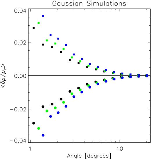
Fig. 3 presents the ensemble-averaged results obtained from 5000 Gaussian Monte Carlo realizations. As expected, for the three adopted thresholds, overdensities (or positive excursions in the projected density map) yield a positive signal for the stacked aperture analysis (as displayed by the squares in the plots), whereas underdensities yield negative ones (circles in the plot). The Monte Carlo realizations also enable us to compute the variance on the measurements. On taking the ratio of the mean signal and the rms noise, we obtain direct estimates of the |${\mathcal {S}}/{\mathcal {N}}$| for each given aperture bin. The coloured solid lines in the plot present our direct measurements of the |${\mathcal {S}}/{\mathcal {N}}$|⁠. Thus, we clearly see that the scatter induced by the CMB generated at z ≃ 1050 is the dominant source of noise, keeping the |${\mathcal {S}}/{\mathcal {N}}$| for each angular bin below unity.

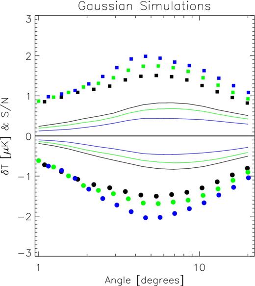
$AP filter outputs for the Gaussian realizations of the V band of WMAP. Results for realizations of other bands are virtually identical to these. The black, green and blue symbols and curves refer to density threshold choices of ν = 2.5, 2.8 and 3.2, respectively. Circles correspond to voids and squares to superclusters, while solid lines display the $\mathcal {S}/\mathcal {N}$ at each scale.$

Figure 3.

AP filter outputs for the Gaussian realizations of the V band of WMAP. Results for realizations of other bands are virtually identical to these. The black, green and blue symbols and curves refer to density threshold choices of ν = 2.5, 2.8 and 3.2, respectively. Circles correspond to voids and squares to superclusters, while solid lines display the |$\mathcal {S}/\mathcal {N}$| at each scale.

Open in new tab Download slide

For lower thresholds there is more area covered and intuitively one would expect a higher |${\mathcal {S}}/{\mathcal {N}}$|⁠, as it seems to be the case. Our realizations also provide higher ISW amplitudes for higher thresholds, and this makes sense since deeper voids/potential wells should have a stronger impact on CMB photons. Nevertheless, in all cases typical amplitudes remain at the level of 1–2 μK. The aperture at which the AP outputs provide the highest amplitude does not show any strong dependence upon the threshold ν, and seems to lie in a wide angle range within [3°, 8°]. For apertures larger than 10°, the |${\mathcal {S}}/{\mathcal {N}}$| for the lowest threshold starts dropping slowly and becomes half of its maximum value at an aperture of 20°. For higher thresholds this decrease is found to be even shallower.

4.2 Generation of non-linear ISW and density maps from N-body simulations

The previous sub-section has shown that the Gaussian realizations of the ΛCDM universe are in tension with the excess signal found by G08. One weak point in the above analysis is that the density and late-time potential field are not necessarily well described by a Gaussian process, since non-linear evolution under gravity drives the initially Gaussian distribution of density fluctuations towards one that is non-Gaussian at late times. In order to test whether non-linear evolution could explain the excess signal seen by G08, we now turn to the challenge of constructing fully non-linear maps of the density field and ISW effect from N-body simulations.

The eight simulations that we employ for this task are a sub-set of the zHORIZON simulations. These simulations were used in Smith et al. (2009) to calculate the expected ISW-cluster cross-power spectra. In brief, each simulation follows the gravitational evolution of N = 750³ dark matter particles in a box of comoving size L = 1500 h⁻¹ Mpc. The cosmological model employed was a flat ΛCDM model: |$\Omega _{\text{m}0}=0.25$|⁠; σ₈ = 0.8; n_s = 1.0; h = 0.72, Ω_{b, 0} = 0.04. The transfer function for the simulations was generated using the cmbfast code (Seljak & Zaldarriaga 1996). The initial conditions were lain down at redshift z = 49 using the code 2lpt (Scoccimarro 1998; Crocce, Pueblas & Scoccimarro 2006). Each initial condition was integrated forward using the publicly available cosmological N-body code gadget-2 (Springel 2005). Snapshots of the phase space were captured at 11 logarithmically spaced intervals between a = 0.5 and a = 1.0.

In order to generate full-sky non-linear ISW maps, we roughly follow the strategy described in Cai et al. (2010), but with some minor changes. Full details of how we construct our maps can be found in Appendix A. In summary, we used the density and divergence of momentum fields to solve for |$\dot{\Phi }$| for each snapshot. We then constructed a backward light-cone from z = 0.0 to z = 1.0 for |$\dot{\Phi }$|⁠. We then pixelated the sphere using the healpix equal-area decomposition, taking the pixel resolution to be N_side = 256, which corresponds to 786,432 pixels on the sphere. For each pixel location, we then fired a ray through the past light-cone of |$\dot{\Phi }$| and accumulated the line-of-sight integral given by equation (1). Note that we only consider the ISW signal coming from z < 1, since we do not expect a significant cross-correlation between the relatively low-redshift density slices for SDSS and the ISW from z > 1. The top panel of Fig. 4 shows one of the ISW maps that we have generated from the zHORIZON simulations.

Figure 4.

Top panel: full-sky, non-linear ISW map arising from structures between z = 0.0 and z = 1.0, estimated from one of the zHORIZON simulations. The sky map was pixelated using the healpix package with a resolution of N_side = 256, which corresponds to 786 432 pixels. Bottom panel: full-sky projected overdensity map for the distribution of CDM structures located in the redshift shell z = [0.260, 0.366] for the same N-body simulation. The map was pixelated at the same resolution as the ISW map and smoothed with a Gaussian filter of scale FWHM = 16.9 arcmins (roughly the angular size subtended by 1 h⁻¹ Mpc at z = 0.3). In both panels, the graticule scale indicates 30°divisions.

Open in new tab Download slide

We next generated the projected density maps. These were done by first constructing the projected density map associated with each snapshot a_i. The density field for a given snapshot was obtained as follows. To each snapshot a_l, we associate a specific comoving shell [χ_l−1/2, χ_l+1/2] (see Appendix A for more details). We then select all of the particles that fall into the shell for that epoch, i.e. the ith dark matter particle in the a_lth snapshot, is accepted in the shell if |$\chi _{l-1/2}<|{\boldsymbol x}_{\rm i}-{\boldsymbol x}_{\rm O}|\le \chi _{l+1/2}$|⁠, where |${\boldsymbol x}_{\rm i}$| and |${\boldsymbol x}_{\rm O}$| are the coordinates of the ith dark matter particle and the observer, respectively. Note that if a given value of χ is larger than L/2, 3L/2, 5L/2, …, then we apply periodic boundary conditions to produce replications of the cube to larger distances. If the particle is accepted, then we compute the angular coordinates (θ, ϕ) for the particle, relative to the observer. Given these angular coordinates, we then find the associated healpix pixel and increment the counts in that pixel. The bottom panel of Fig. 4 shows the projected overdensity map for a thin redshift shell centred on z = 0.3. We note that it is hard, by eye, to note any apparent correspondence between the overdensity and temperature maps.

At the end, we have 11 density maps between z = 1.0 and z = 0.0 that form concentric shells around the observer. These shells were then co-added using the weights given by our analytic fit to the redshift distribution of superclusters and supervoids (recall the solid line in the left-hand panel of Fig. 1). The resulting co-added all-sky density maps are then smoothed from N_side = 256 to N_side = 32, and the positions of the 2n, n and n/2 most underdense and overdense pixels on this map are recorded. The number n corresponds to a number density of extrema that is identical to that of real voids and superclusters under the footprint of SDSS DR6. Each of those extreme pixels on the N_side = 32 map is then projected back to the N_side = 256 map on a sub-set of 64 higher resolution pixels, out of which the position of the most underdense or overdense pixel is used as the target of the AP filter.

4.3 Validation tests of zHORIZON derived maps

Before we apply the analysis methods of G08 to our ISW and density maps, we first test the consistency of the maps themselves. To do this, we compute the angular autopower spectra of the ISW temperature maps for each of the eight zHORIZON runs. The left-hand panel of Fig. 5 presents the ensemble-averaged temperature power spectrum for the ISW effect. The measurements from the simulations are represented by the solid black points. The prediction from linear theory is given by the solid red line. For multipoles in the range 5 < ℓ < 70, the agreement between the two is excellent. At low multipoles (ℓ < 5), the absence of power in the simulation on scales larger than L induces a low bias. Instead, on scales ℓ > 70, the non-linear evolution of potentials substantially boosts the signal relative to linear by means of the Rees–Sciama effect.

Figure 5.

Left: comparison of the average angular power spectra obtained from the zHORIZON-derived ISW maps (black circles) and the theoretical expectation (red solid line). The lack of low-k modes causes a low bias in the low multipole range, and non-linear evolution introduces some visible power excess on the small scales. Middle: comparison of the average angular power spectra from the zHORIZON-derived density contrast maps (black circles) with the linear prediction (red solid line), for the redshift range z ∈ [0.1, 1]. The agreement with theory is again good on intermediate and small scales, but there seems to be again some slight low bias on the largest scales/lowest multipoles. Right: comparison of the average cross-angular power spectra from the zHORIZON-derived density and ISW maps and the linear theory prediction (red solid line), for the redshift range z ∈ [0.1, 1.]. Data from the simulations compare low to theoretical expectations on the large scales/low multipoles due to the finite box size, on the high multipoles due to non-linear evolution, and also show a slight (∼10 per cent) power deficit on intermediate multipoles due to the finite discretization of the line of sight into 11 shells.

Open in new tab Download slide

We next compute the angular autopower spectrum of the projected density contrast maps, with the projection extending from z = 0.1 to z = 1 (middle panel of Fig. 5). In this case, the projected density angular power spectrum shows good agreement with the linear theory expectations in the intermediate- and high-multipole range (5 < ℓ < 200), and some hints for power deficit on the large scales/low ℓ-s, which would probably be due to the lack of k modes beyond the box size of the simulations.

Finally, the right-hand panel of Fig. 5 compares the ISW – density cross-correlation estimated from the simulations with the linear theory. As for the other cases, there exists some power deficit at low multipoles due to finite volume effects in the simulations. At high multipoles, the linear theory prediction lies above the simulations, this owes to the fact that in the deeply non-linear regime potentials do not decay, but grow with time through the Rees–Sciama mechanism, and hence this leads to a suppression of power (for further details see Smith et al. 2009). On intermediate angular scales, the theoretical prediction is roughly ∼10 per cent higher than the simulations, although with significant scatter. This slight mismatch is likely due to the construction of the weighted projected density field, since the ISW auto-spectra are in excellent agreement with the simulations.

4.4 Aperture analysis of the zHORIZON maps

Having validated the simulated maps, we now repeat the AP analysis. Since here we have both full-sky density and temperature maps, we prefer not to apply any sky mask. Thus, these predictions will not be affected by incomplete sky coverage. We repeat the steps described in Section 3 for finding the locations of the density peaks/troughs in each of the simulated smoothed maps. Then, as before, we apply the AP filters to the selected centroid positions for the eight ISW maps from the zHORIZON simulations.

Fig. 6 presents the results from this analysis. The square and circular symbols denote the results for our effective supercluster and supervoid regions, respectively. The blue, green and black colours correspond to the set of extreme pixels which have half, equivalent and double the angular number density of the real supervoids and superclusters found in G08's analysis. We see that the peak of the average AP output has a temperature of the order of 2 μK and occurs for apertures of scale ∼6°–7°.

Figure 6.

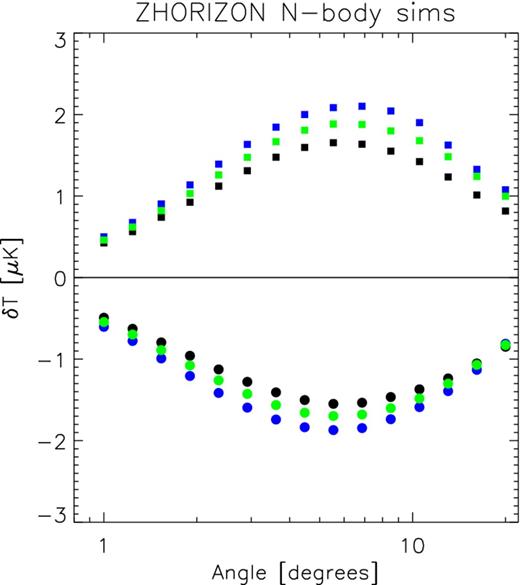
AP filter outputs for ISW maps derived from the zHORIZON simulations. The black, green and blue symbols refer to density excursions in the projected density maps having twice, same and half the angular number density as voids and superclusters from G08. Circles correspond to underdensities and squares to overdensities. These excursions were identified in projected density maps smoothed down to pixels of ∼2 ° on a side (N_side = 32).

Open in new tab Download slide

On comparison with the predictions from our Gaussian realizations, we find that the fully non-linear ISW maps are in close agreement (cf. Section 4.1). There are however small differences. The peak signal is shifted to slightly larger scales for the full non-linear case. Also, the shape of the curves obtained from the zHORIZON simulations appears smoother than in the Gaussian simulation case, which shows dips and troughs that are absent in Fig. 6. We believe that these small differences are likely a consequence of the fact that the Gaussian realizations include intrinsic CMB noise and possess a sky mask.

Actually, after applying the real sky masks to the simulated maps, we find that the peak amplitudes and the general shapes of the functions in Fig. 6 become distorted at the ∼10 per cent level.

However, the most important point to note, is that on angular scales of the order of 3°–4°, the Gaussian and fully non-linear simulations are in close agreement: the difference induced by adopting a slightly different cosmological model should introduce changes in the ISW amplitude at the 2 per cent level, and the ISW generated beyond z = 1 seems to have little impact as well. We thus conclude this section by noting that that the excess temperature signal found by G08, and now confirmed by us in Section 3, appears to be incompatible with the evolution of gravitational potentials in the standard ΛCDM model. Our results from both Gaussian realizations and ISW maps derived from the N-body simulations are in agreement with Granett et al. (2009), who found no signature at the few degree scale on voids and clusters with the amplitude found on real WMAP data when producing an ISW map out of the distribution of LRG in Sloan data.

5 SIGNIFICANCE, SYSTEMATICS AND ALTERNATIVE MODELS

5.1 Estimating the significance

The direct comparison of Figs 2 and 3 reveals clear differences between the observed data and theoretical predictions. Not only is the amplitude of the maximum signal in the real data a factor of ∼5 times larger than the average in the Gaussian realizations, but the dependence of the signal on the filter scale shows a different shape. More quantitatively, the results from the W-band WMAP data for an aperture size of 3| $_{.}^{\circ}$|6, are of the order of ∼3.4σ away from the supervoid simulation average, and ∼2.1σ away from the average for the case of superclusters. In terms of probability, for an aperture scale of 3| $_{.}^{\circ}$|6, only 5 out of the 5000 realizations possessed an ISW signal, from supervoid regions, with a temperature decrement lower than the one found in real data, and 97 of the realizations for superclusters exceeded the value obtained for the real data. Taken at face value, this analysis seems to exclude the Gaussian ΛCDM hypothesis at ∼4σ significance. However, this is an a posteriori estimate, since we have neglected the fact that we also looked for a signal at other aperture scales.

If, for the W-band WMAP data, we include the measurements from the 15 different angular aperture scales between 1°and 20°and take into account their covariance, then the significance drops. Under the assumption of Gaussian statistics, we find that the WMAP outputs for voids produce a |$\chi ^2_{\rm voids}=23.5$| (n_d.o.f. = 15). The corresponding figure for superclusters is |$\chi ^2_{\rm superclusters}=26.6$| (n_d.o.f. = 15). If we treat these two constraints as being independent then their combination yields |$\chi ^2_{\rm both}=50.0$| (n_d.o.f. = 30). In terms of probability, this means that the WMAP data have a 0.012 probability (i.e. <2 per cent chance or ∼2.2σ under Gaussian statistics) of being consistent with the evolution of gravitational potentials in the ΛCDM model. If we consider the null hypothesis of no ISW signatures expected at all (for which stacking on voids and superclusters should leave no temperature decrement/increment), then the results lie at 2.6 σ away from this scenario.

We next study the dependence of the statistical significance on the number of sub-structures considered in the analysis. While the original catalogue of voids and superclusters of G08 contains 50 entries, we now repeat our tests after considering two sub-samples containing only the first 30 and 40 objects. For these sub-samples, the adopted values of the Gaussian threshold were ν = 2.87 and 2.97. In these cases, the pattern found for the full catalogue is reproduced: the stacked voids give a temperature decrement of ≲ −10 μK, at ∼3–3.5σ; the stacked superclusters give a temperature increment of ≳ 7 μK, at the level of ∼2.2–2.4σ. On comparison with Gaussian realizations, we find that, after considering all aperture radii, results for the first 40 superstructures are in lower tension with the outputs of Gaussian realizations (at the level of <3.0 per cent or 1.9σ). This level of tension further decreases when considering only the first 30 superstructures (∼27 per cent or 0.6σ), showing that the tension of WMAP data with respect to Gaussian realizations relaxes as fewer structures are included in the analysis. This is somehow expected from the Gaussian realizations, for which the statistical significance for the ISW increases with decreasing thresholds. This is in apparent contradiction with table 1 of G08, where it is shown that the statistical significance of their ISW measurement at a scale of 4°decreases when increasing the number of structures from 50 (4.4σ) to 70 (2.8σ). In G08, it is argued that by considering more structures one may be diluting the signal by including unphysical structures, an extent that cannot be tested in our Gaussian maps since it is strictly associated with the algorithms identifying voids and superclusters in the galaxy catalogues.

In summary, according to our Gaussian simulations, the ∼4σ deviation with respect to ΛCDM expectations found at ∼4° aperture radius decreases to ∼2.2σ when including different filter apertures in the range [1°, 20°], and lies, in this case, 2.6σ away from the null (no ISW) case. While this tension relaxes when considering fewer structures, the significance of the detected signal seems to decrease when considering more than 50 voids and superclusters (see table 1 of G08), in an opposite trend to what is suggested by our Gaussian ISW realizations.

We conclude that most of the significance of the G08 result is at odds with ISW ΛCDM predictions, both in amplitude and scale/aperture radius dependence, and that this tension considerably reduces when more aperture radii and structure sub-samples are considered in the analysis.

5.2 Tests for systematics

Given the high level of discrepancy existing between the pattern found at 3| $_{.}^{\circ}$|6 aperture radius and ISW ΛCDM expectations, we next test the possibility of systematics in WMAP data giving rise to the observed signal.

Rotation test: we first conduct a rotation test assessing the statistical significance of the AP outputs for a 3| $_{.}^{\circ}$|6 scale. In this way, we probe the possibility of any other signal (apart from CMB) contributing to the uncertainty of the AP filter outputs and hence modifying the statistical significance found for WMAP data. We rotate in galactic longitude (in steps of 9°) the AP filter targets with respect to the real positions of supervoids and superclusters. In the absence of systematics, this should provide AP outputs compatible with zero.
Fig. 7 presents the results from this analysis. The blue circular symbols represent the supervoid regions and the red square symbols denote the superclusters. At zero rotation lag, we clearly obtain a signal of higher amplitude than in any other rotation bin. We have verified that this signal does not arise as a consequence of a small sub-set of the supervoids/superclusters. Instead, the signal is approximately evenly distributed among all structures. From the sample of rotated bins only, the estimated significance for the 3| $_{.}^{\circ}$|6 aperture is 4.1σ for voids, 2.7σ for superclusters and 3.8σ combined. This is within 1σ from the significance levels obtained with the Gaussian realizations.
Density-dependent contaminant: another possible systematic is some combination of contaminants present in the superclusters that increases the emission in these structures in a frequency-independent manner. This could happen if the CMB cleaning algorithms remove only the frequency varying part of the contaminant signal, but leave behind a DC level. In such a scenario, one might assume that the signal is linearly responding to fluctuations in the projected matter density. We incorporate this effect into our Gaussian realizations by substituting the total CMB map by a signal that is proportional to the projected matter density field in our Gaussian realizations. This should provide us with some idea of the scale dependence for a contaminant of this nature.
Fig. 8, presents the results from this exercise. The symbol styles and point colours are the same as in Fig. 3. The recovered shape resembles that for a standard matter autocorrelation function and is remarkably different from that of Fig. 2. Actually, the profile from real data in Fig. 2 seems to be an intermediate case between the scenario depicted in Fig. 8 and the theoretical predictions of Fig. 3. However, if most of the observed amplitude at 3| $_{.}^{\circ}$|6 ( ∼ 8 − 2 = 6 μK out of the total ∼ 8 μK observed) is to be caused by this type of contaminant, then the scale dependence of the output should accordingly be much closer to the one shown in Fig. 8, and this is not the case. Note that we have assigned ∼ 2 μK to ISW in this estimation. If contaminants in the position of the AP targets were Poisson distributed, then the profiles obtained in Fig. 8 would approach zero faster as aperture radii increase, yet in stronger disagreement with Fig. 2.
Superstructure selection effects: It might be argued that our identification of underdense and overdense regions in our simulated density maps does not match well the selection of supervoids and superclusters in the G08 data. Whilst in principle both approaches should generate the most underdense and overdense regions in volume limited samples of the universe, differences in the exact details of the ZOBOV and VOBOZ implementations may introduce subtle but important differences in the selection of regions. This would have an impact in the final definition and selection of targets for the AP filters. Properly addressing this issue would require a thorough implementation of the ZOBOV and VOBOZ algorithms to semi-analytic galaxy samples embedded in our simulations (and this goes beyond the scope of this work). Having said this, the stability of our results with respect to the actual density peak threshold adopted, suggests that this would not critically affect our conclusions.

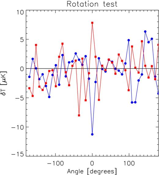
$Rotation test on AP filter outputs for an aperture size of 3 $_{.}^{\circ}$6. The blue circles (red squares) correspond to voids (superclusters).$

Figure 7.

Rotation test on AP filter outputs for an aperture size of 3| $_{.}^{\circ}$|6. The blue circles (red squares) correspond to voids (superclusters).

Open in new tab Download slide

Figure 8.

Pattern induced versus AP filter scale by a contaminant following the local matter density.

Open in new tab Download slide

5.3 Primordial non-Gaussianity

In this section, we explore whether the G08 result is compatible with a non-Gaussian distribution for the primordial potential perturbations. In particular, we consider the well-known local model for primordial non-Gaussianity, characterized by a quadratic correction to the Gauge invariant Bardeen's potential perturbation (see Komatsu et al. 2011, and references therein):

\begin{equation} {\rm \Phi }_{\rm NG}({\boldsymbol x})={\rm \Phi }_{\rm G}({\boldsymbol x})+ {f_{\rm NL}^{\rm local}}\left[{\rm \Phi }_{\rm G}({\boldsymbol x})^2-\left\langle {\rm \Phi }_{\rm G}^2({\boldsymbol x})\right\rangle \right]\,, \end{equation}

(9)

where Φ_G(x) is the Gaussian potential perturbation after matter radiation equality, scaled in terms of units of c² to yield a dimensionless quantity. Following standard convention, |${\rm \Phi }_{\rm NG}({\boldsymbol x})\equiv -\Phi ^{\rm Newton}({\boldsymbol x})$| (i.e. the Φ in equation (1)). The term |$\langle{\rm \Phi }_{\rm G}^2(x)\rangle$| is subtracted to ensure that Φ_NG is a mean zero field. In linear theory, the typical fluctuations are of the order of Φ_NG ∼ 10⁻⁵, and so the non-Gaussian corrections are of the order of |${\sim }0.1\ \mathrm{per\ cent}\ ({f_{\rm NL}^{\rm local}}/100)({\rm \Phi }_{\rm G}/10^{-5})^2$|⁠.

In order to explore the observable consequences of such a modification, we have generated a set of simulated ISW maps with Gaussian initial conditions, i.e. |${f_{\rm NL}^{\rm local}}=0$|⁠, and with non-Gaussian initial conditions |${f_{\rm NL}^{\rm local}}=\lbrace +100,-100\rbrace$|⁠. These maps were generated from N-body simulations seeded with Gaussian and non-Gaussian initial conditions following the methodology of Appendix A. The simulations that we employ were fully described in Desjacques, Seljak & Iliev (2009). In brief, these were performed using gadget-2, and followed N = 1024³ dark matter particles in a box of size L = 1600 h⁻¹ Mpc. The cosmological model of the simulations was consistent with the WMAP5 data (Komatsu et al. 2009). We use a sub-set of these simulations that were used elsewhere for gravitational lensing analysis (Marian et al. 2011; Hilbert et al. 2012). The simulations were set up to have the same initial random phases for all three models, this enables us to cancel some of the cosmic variance and so permits us to better explore the model differences.

The top panel of Fig. 9 presents the differences between the ISW temperature maps in a universe with |${f_{\rm NL}^{\rm local}}=+100$| and |${f_{\rm NL}^{\rm local}}=0$|⁠. The bottom panel shows the same but for the case |${f_{\rm NL}^{\rm local}}=-100$| and |${f_{\rm NL}^{\rm local}}=0$|⁠. Note that all of the maps were smoothed with a Gaussian filter of FWHM = 1° before being differenced. Note also that we have only included the ISW contributions between z = 0.0 and z = 1.0. Clearly, the presence of primordial non-Gaussianities can induce shifts in the temperatures of the peaks and troughs of the distribution. However, these shifts are modest for |${f_{\rm NL}^{\rm local}}=\pm 100$|⁠, leading to changes that are < 1μK. This suggests that values of |${f_{\rm NL}^{\rm local}}$| of the order of ∼1000, might be able to explain the AP analysis of the WMAP results. However, such large values for |${f_{\rm NL}^{\rm local}}$| would be grossly inconsistent with the values of |${f_{\rm NL}^{\rm local}}$| obtained from the CMB temperature bispectrum, which currently gives |$-10<f_{\rm NL}^{\rm local} <74$| (95 per cent CL, Komatsu et al. 2011). It therefore seems unlikely that the scale-independent local model of primordial non-Gaussianity is the correct explanation for the excess signal.

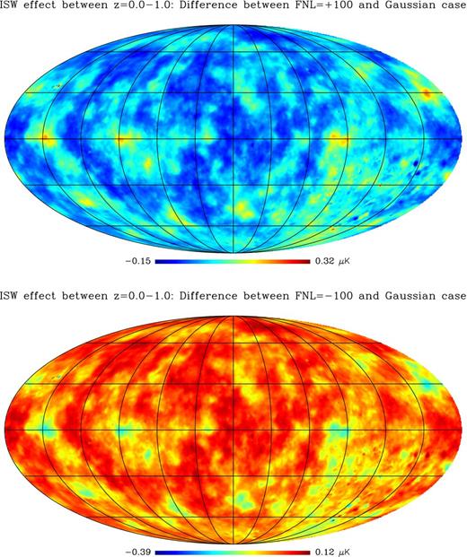
$Relative difference between full-sky ISW temperature maps for models with primordial non-Gaussianity and Gaussian models for flat ΛCDM universes. Top panel: presents $\Delta T^{\rm ISW}({f_{\rm NL}^{\rm local}}=+100)-\Delta T^{\rm ISW}({f_{\rm NL}^{\rm local}}=0)$. Bottom panel: presents the same but for $\Delta T^{\rm ISW}({f_{\rm NL}^{\rm local}}=-100)-\Delta T^{\rm ISW}({f_{\rm NL}^{\rm local}}=0)$. All maps were smoothed with a Gaussian filter of FWHM = 1 $_{.}^{\circ}$0, which roughly corresponds to the scales at which the signal for the AP filters peaks. The large-scale temperature fluctuations appear slightly cooler/hotter in universes with ${f_{\rm NL}^{\rm local}}$ positive/negative.$

Figure 9.

Relative difference between full-sky ISW temperature maps for models with primordial non-Gaussianity and Gaussian models for flat ΛCDM universes. Top panel: presents |$\Delta T^{\rm ISW}({f_{\rm NL}^{\rm local}}=+100)-\Delta T^{\rm ISW}({f_{\rm NL}^{\rm local}}=0)$|⁠. Bottom panel: presents the same but for |$\Delta T^{\rm ISW}({f_{\rm NL}^{\rm local}}=-100)-\Delta T^{\rm ISW}({f_{\rm NL}^{\rm local}}=0)$|⁠. All maps were smoothed with a Gaussian filter of FWHM = 1| $_{.}^{\circ}$|0, which roughly corresponds to the scales at which the signal for the AP filters peaks. The large-scale temperature fluctuations appear slightly cooler/hotter in universes with |${f_{\rm NL}^{\rm local}}$| positive/negative.

Open in new tab Download slide

6 CONCLUSIONS

In this work, we have studied the imprint of superclusters and supervoids in the temperature map of the CMB from the WMAP experiment. Our work further explores the signature first detected in G08.

In Section 2, we theoretically showed that if G08 had applied a standard angular cross-power spectrum analysis of the superstructures they found in the SDSS LRG data, then the expected significance for a ΛCDM model should have been <1.5σ.

In Section 3, we cross-checked the G08 analysis directly and found identical conclusions: on scales ∼3| $_{.}^{\circ}$|6 there was a ∼4σ detection significance for excess signal associated with the supervoids and superclusters.

In Section 4, we performed a series of tests exploring whether these findings are consistent with the standard ΛCDM model. Gaussian Monte Carlo realizations of the ISW effect and the LSS were unable to produce such large signals. We then investigated whether this was a consequence of our simplified Gaussian realizations. We did this by generating fully non-linear ISW maps from large volume N-body simulations. These simulated maps confirmed the findings of the simpler Gaussian realizations.

In Section 5, we used the Gaussian Monte Carlo realizations to explore the significance of the deviations from the ΛCDM model found in the WMAP data. We found that for AP analysis of the maps on scales 3| $_{.}^{\circ}$|6, results from WMAP data are lying about ∼4σ away from ΛCDM expectations. However, on taking into account the 15 aperture scales examined, the significance of the discrepancy dropped to <2 per cent chance (2.2σ) of the result being consistent with the ΛCDM model. In this case, results remained 2.6σ away from the null (ISW-free) scenario where structures leave no signatures on the CMB at the linear level. When including fewer structures in the analysis, the tension dropped further, and results for only 30 voids and superclusters were compatible both with ΛCDM expectations (at 0.6σ) and the null (no ISW) scenario (at 1.3σ). Our simulations also suggested that the ISW significance should increase when more structures were included in the analysis, in apparent contradiction with the findings of G08. Hence, most of the detected signal appeared associated with the full set of 50 superstructures and an aperture radius of 3| $_{.}^{\circ}$|6.

We investigated whether the observed pattern at a radius of 3| $_{.}^{\circ}$|6 could be caused by a systematic error in the cleaning of foregrounds in the WMAP data. We found that if the signal were to be caused by an approximately frequency-independent emission tracing the density field, then the resulting angular dependence would be very different to the measured shape found in the WMAP data.

We next explored whether the observed signal at 3| $_{.}^{\circ}$|6 could be generated by primordial non-Gaussianities. We considered the local model, characterized by a quadratic correction to the primordial potential perturbations, with the coupling parameter |${f_{\rm NL}^{\rm local}}$|⁠. We found that, for |${f_{\rm NL}^{\rm local}}$| positive/negative, asymmetric shifts in ISW temperature maps arise. However, for the values of |${f_{\rm NL}^{\rm local}}=\pm 100$|⁠, the changes were < 1μK (after smoothing the maps down to degree scales). Thus, values of |${f_{\rm NL}^{\rm local}}$| an order of magnitude higher would be required to explain the G08 result, and they would be clearly inconsistent with current constraints on |${f_{\rm NL}^{\rm local}}$| from WMAP.

It is possible that the G08 result may also be explained by other more exotic scenarios, e.g. non-Gaussianity arising from the presence of a non-zero primordial equilateral or orthogonal model bispectrum (a consequence of non-standard inflationary mechanisms); alternatively it might arise as a direct consequence of modifications to Einstein's general theory of relativity, (Jain & Khoury 2010). However, more conservative scenarios involving some combination of artefacts and/or systematics cannot yet be fully discarded.

In the future, we will look with interest to the results from the Planck satellite as to whether this signal represents a data artefact, or whether it constitutes a genuine challenge to the ΛCDM model and a window to new cosmological physics.

It is a pleasure to acknowledge Raúl Angulo, Jose María Diego, Marian Douspis, Benjamin Granett, S. Illic and István Szapudi for useful discussions. We also thank Laura Marian for carefully reading the manuscript. We kindly thank Vincent Desjacques for providing us with access to his non-Gaussian realizations. C.H-M. is a Ramón y Cajal fellow of the Spanish Ministry of Economy and Competitiveness. The work of RES was supported by Advanced Grant 246797 ‘GALFORMOD’ from the European Research Council. We acknowledge the use of the healpix package (Górski et al. 2005) and the lambda data base. We thank Volker Springel for making public his code gadget-2, and Roman Scoccimarro for making public his 2lpt code. We acknowledge the ITP, University of Zürich for providing assistance with computing resources.

1

http://map.gsfc.nasa.gov

2

http://skysrv.pha.jhu.edu/~neyrinck/voboz/

3

http://ifa.hawaii.edu/cosmowave/supervoids/

4

http://lambda.gsfc.nasa.gov

5

URL site: http://healpix.jpg.nasa.gov.

REFERENCES

Adelman-McCarthy

J. K.

The SDSS Team

,

ApJS

,

2008

, vol.

175

pg.

297

Crossref

Search ADS

Afshordi

N.

Loh

Y.-S.

Strauss

M. A.

,

Phys. Rev. D

,

2004

, vol.

69

pg.

083524

Crossref

Search ADS

Bielby

R.

Shanks

T.

Sawangwit

U.

Croom

S. M.

Ross

N. P.

Wake

D. A.

,

MNRAS

,

2010

, vol.

403

pg.

1261

Crossref

Search ADS

Boughn

S.

Crittenden

R.

,

Nat

,

2004

, vol.

427

pg.

45

Crossref

Search ADS

Cabré

A.

Gaztañaga

E.

Manera

M.

Fosalba

P.

Castander

F.

,

MNRAS

,

2006

, vol.

372

pg.

L23

Crossref

Search ADS

Cai

Y.-C.

Cole

S.

Jenkins

A.

Frenk

C.

,

MNRAS

,

2009

, vol.

396

pg.

772

Crossref

Search ADS

Cai

Y.-C.

Cole

S.

Jenkins

A.

Frenk

C. S.

,

MNRAS

,

2010

, vol.

407

pg.

201

Crossref

Search ADS

Cole

S.

The 2dFGRS Team

,

MNRAS

,

2005

, vol.

362

pg.

505

Crossref

Search ADS

Crittenden

R. G.

Turok

N.

,

Phys. Rev. Lett.

,

1996

, vol.

76

pg.

575

Crossref

Search ADS

PubMed

Crocce

M.

Pueblas

S.

Scoccimarro

R.

,

MNRAS

,

2006

, vol.

373

pg.

369

Crossref

Search ADS

Desjacques

V.

Seljak

U.

Iliev

I. T.

,

MNRAS

,

2009

, vol.

396

pg.

85

Crossref

Search ADS

Dodelson

S.

,

Modern cosmology

,

2003

Amsterdam

Academic Press

pg.

XIII, 440

Google Scholar

Google Preview

OpenURL Placeholder Text

WorldCat

Flender

S.

Hotchkiss

S.

Nadathur

S.

,

J. Cosmol. Astropart. Phys.

,

2013

, vol.

2

pg.

13

Crossref

Search ADS

Fosalba

P.

Gaztañaga

E.

,

MNRAS

,

2004

, vol.

350

pg.

L37

Crossref

Search ADS

Fosalba

P.

Gaztañaga

E.

Castander

F. J.

,

ApJ

,

2003

, vol.

597

pg.

L89

Crossref

Search ADS

Francis

C. L.

Peacock

J. A.

,

MNRAS

,

2010

, vol.

406

pg.

2

Crossref

Search ADS

Giannantonio

T.

Crittenden

R.

Nichol

R.

Ross

A. J.

,

MNRAS

,

2012

, vol.

426

pg.

2581

Crossref

Search ADS

Giannantonio

T.

et al. ,

Phys. Rev. D

,

2006

, vol.

74

pg.

063520

Crossref

Search ADS

Gold

B.

The WMAP Team

,

ApJS

,

2011

, vol.

192

pg.

15

Crossref

Search ADS

Górski

K. M.

Hivon

E.

Banday

A. J.

Wandelt

B. D.

Hansen

F. K.

Reinecke

M.

Bartelmann

M.

,

ApJ

,

2005

, vol.

622

pg.

759

Crossref

Search ADS

Granett

B. R.

Neyrinck

M. C.

Szapudi

I.

,

ApJ

,

2008

, vol.

683

pg.

L99

G08

Crossref

Search ADS

Granett

B. R.

Neyrinck

M. C.

Szapudi

I.

,

ApJ

,

2009

, vol.

701

pg.

414

Crossref

Search ADS

Hernández-Monteagudo

C.

,

A&A

,

2008

, vol.

490

pg.

15

Crossref

Search ADS

Hernández-Monteagudo

C.

,

A&A

,

2010

, vol.

520

pg.

A101

Crossref

Search ADS

Hernández-Monteagudo

C.

Génova-Santos

R.

Atrio-Barandela

F.

Mornas

L.

Diaz Alonso

J.

,

AIP Conf. Proc. Vol. 841, Is there Any Evidence for Integrated Sachs-Wolfe Signal in WMAP First Year Data?

,

2006

New York

Am. Inst. Phys.

pg.

389

Google Scholar

Google Preview

OpenURL Placeholder Text

WorldCat

Hilbert

S.

Marian

L.

Smith

R. E.

Desjacques

V.

,

MNRAS

,

2012

, vol.

426

pg.

2870

Crossref

Search ADS

Ho

S.

Hirata

C.

Padmanabhan

N.

Seljak

U.

Bahcall

N.

,

Phys. Rev. D

,

2008

, vol.

78

pg.

043519

Crossref

Search ADS

Hockney

R. W.

Eastwood

J. W.

,

Computer Simulation Using Particles

,

1988

Hilger

Bristol

Google Scholar

Google Preview

OpenURL Placeholder Text

WorldCat

Inoue

K. T.

,

MNRAS

,

2012

, vol.

421

pg.

2731

Crossref

Search ADS

Inoue

K. T.

Sakai

N.

Tomita

K.

,

ApJ

,

2010

, vol.

724

pg.

12

Crossref

Search ADS

Jain

B.

Khoury

J.

,

Ann. Phys.

,

2010

, vol.

325

pg.

1479

Crossref

Search ADS

Jarosik

N.

et al. ,

ApJS

,

2011

, vol.

192

pg.

14

Crossref

Search ADS

Johnson

S.

Frigo

M.

,

2008

available at: http://www.fftw.org/

Komatsu

E.

The WMAP Team

,

ApJS

,

2009

, vol.

180

pg.

330

Crossref

Search ADS

Komatsu

E.

Smith

K. M.

Dunkley

J.

The WMAP Team

,

ApJS

,

2011

, vol.

192

pg.

18

Crossref

Search ADS

López-Corredoira

M.

Sylos Labini

F.

Betancort-Rijo

J.

,

A&A

,

2010

, vol.

513

pg.

A3

Crossref

Search ADS

Marian

L.

Hilbert

S.

Smith

R. E.

Schneider

P.

Desjacques

V.

,

ApJ

,

2011

, vol.

728

pg.

L13

Crossref

Search ADS

McEwen

J. D.

Vielva

P.

Hobson

M. P.

Martínez-González

E.

Lasenby

A. N.

,

MNRAS

,

2007

, vol.

376

pg.

1211

Crossref

Search ADS

Nadathur

S.

Hotchkiss

S.

Sarkar

S.

,

J. Cosmol. Astropart. Phys.

,

2012

, vol.

6

pg.

42

Crossref

Search ADS

Neyrinck

M. C.

,

MNRAS

,

2008

, vol.

386

pg.

2101

Crossref

Search ADS

Neyrinck

M. C.

Gnedin

N. Y.

Hamilton

A. J. S.

,

MNRAS

,

2005

, vol.

356

pg.

1222

Crossref

Search ADS

Nolta

M. R.

et al. ,

ApJ

,

2004

, vol.

608

pg.

10

Crossref

Search ADS

Padmanabhan

N.

Hirata

C. M.

Seljak

U.

Schlegel

D. J.

Brinkmann

J.

Schneider

D. P.

,

Phys. Rev. D

,

2005

, vol.

72

pg.

043525

Crossref

Search ADS

Pápai

P.

Szapudi

I.

,

ApJ

,

2010

, vol.

725

pg.

2078

Crossref

Search ADS

Pápai

P.

Szapudi

I.

Granett

B. R.

,

ApJ

,

2011

, vol.

732

pg.

27

Crossref

Search ADS

Peebles

P. J. E.

,

Research Supported by the National Science Foundation

,

1980

Princeton, NJ

Princeton Univ. Press

pg.

435

Google Scholar

Google Preview

OpenURL Placeholder Text

WorldCat

Perlmutter

S.

Aldering

G.

The Supernova Cosmology Project Team

,

ApJ

,

1999

, vol.

517

pg.

565

Crossref

Search ADS

Rassat

A.

Land

K.

Lahav

O.

Abdalla

F. B.

,

MNRAS

,

2007

, vol.

377

pg.

1085

Crossref

Search ADS

Rees

M. J.

Sciama

D. W.

,

Nat

,

1968

, vol.

217

pg.

511

Crossref

Search ADS

Riess

A. G.

Filippenko

A. V.

The High-z Supernovae Team

,

AJ

,

1998

, vol.

116

pg.

1009

Crossref

Search ADS

Sachs

R. K.

Wolfe

A. M.

,

ApJ

,

1967

, vol.

147

pg.

73

Crossref

Search ADS

Scoccimarro

R.

,

MNRAS

,

1998

, vol.

299

pg.

1097

Crossref

Search ADS

Scranton

R.

et al. ,

2003

preprint (arXiv:e-prints)

Seljak

U.

,

ApJ

,

1996

, vol.

460

pg.

549

Crossref

Search ADS

Seljak

U.

Zaldarriaga

M.

,

ApJ

,

1996

, vol.

469

pg.

437

Crossref

Search ADS

Smith

R. E.

Scoccimarro

R.

Sheth

R. K.

,

Phys. Rev. D

,

2007

, vol.

75

pg.

063512

Crossref

Search ADS

Smith

R. E.

Hernández-Monteagudo

C.

Seljak

U.

,

Phys. Rev. D

,

2009

, vol.

80

pg.

063528

Crossref

Search ADS

Spergel

D. N.

The WMAP Team

,

ApJS

,

2003

, vol.

148

pg.

175

Crossref

Search ADS

Spergel

D. N.

The WMAP Team

,

ApJS

,

2007

, vol.

170

pg.

377

Crossref

Search ADS

Springel

V.

,

MNRAS

,

2005

, vol.

364

pg.

1105

Crossref

Search ADS

Tegmark

M.

The SDSS Team

,

Phys. Rev. D

,

2006

, vol.

74

pg.

123507

Crossref

Search ADS

The Planck Collaboration

,

2006

preprint (astro-ph/0604069)

Thomas

S. A.

Abdalla

F. B.

Lahav

O.

,

Phys. Rev. Lett.

,

2011

, vol.

106

pg.

241301

Crossref

Search ADS

PubMed

Vielva

P.

Martínez-González

E.

Tucci

M.

,

MNRAS

,

2006

, vol.

365

pg.

891

Crossref

Search ADS

Weinberg

S.

,

Cosmology

,

2008

Oxford

Oxford Univ. Press

Google Scholar

Google Preview

OpenURL Placeholder Text

WorldCat

APPENDIX A: FULL-SKY ISW MAPS FROM N-BODY SIMULATIONS

In this section, we aim to construct full-sky ISW maps using a suite of N-body simulations. Our approach is similar to that described in Cai et al. (2010), but with some modifications. To be more precise, we aim to compute the line-of-sight integral equation (1), but taking into account the full non-linear evolution of |$\dot{\Phi }$|⁠. The steps we take to achieve this are described below.

A1 Determining |$\dot{\Phi }$|

In order to obtain |$\dot{\Phi }$| directly from the N-body simulations, we make use of equation (4), which tells us that our desired quantity can be determined from knowledge about |$\delta ({\boldsymbol k},a)$| and |$\dot{\delta }({\boldsymbol k},a)$|⁠. In simulations, measuring |$\delta ({\boldsymbol k},a)$| is relatively straightforward, whereas its time derivative is more complicated. As was shown by Seljak (1996), this latter quantity may be obtained from the perturbed continuity equation (Peebles 1980):

\begin{equation} \nabla \cdot \left[1+\delta ({\boldsymbol x};t)\right]{\boldsymbol v}_p({\boldsymbol x};t)=- a(t)\dot{\delta }({\boldsymbol x};t) \,, \end{equation}

(A1)

where |${\boldsymbol v}_p({\boldsymbol x};t)$| is the proper peculiar velocity field. If we define the pseudo-peculiar momentum field to be

\begin{equation} {\boldsymbol p}({\boldsymbol x};t)\equiv \left[1+\delta ({\boldsymbol x};t)\right]{\boldsymbol v}_p({\boldsymbol x};t)\,, \end{equation}

(A2)

then in Fourier space we may solve the continuity equation directly to find

\begin{equation} \dot{\delta }({\boldsymbol k};t)= i{\boldsymbol k}\cdot {\boldsymbol p}({\boldsymbol k};t) /a(t)\,. \end{equation}

(A3)

Hence, our final expression becomes,

\begin{equation} \dot{\Phi }({\boldsymbol k};t) = {\mathcal {F}}(k)\left[ \frac{H(t)}{a(t)}\delta ({\boldsymbol k};t)-\frac{i{\boldsymbol k}\cdot {\boldsymbol p}({\boldsymbol k};t)}{a^2(t)} \right] \,, \end{equation}

(A4)

where we defined the function

\begin{equation} {\mathcal {F}}(k) \equiv \frac{3}{2}\Omega _{\rm m0} \left(\frac{H_0}{k}\right)^2 \,. \end{equation}

(A5)

Thus, in order to estimate |$\dot{\Phi }$|⁠, we simply require estimates of both the density field and pseudo-peculiar momentum field in Fourier space.

The dark matter density field in an N-body simulation can be written as a sum of Dirac delta functions,

\begin{equation} \rho ({\boldsymbol x})= \sum _{l=1}^{N} m_l \delta ^D({\boldsymbol x}-{\boldsymbol x}_l) \,, \end{equation}

(A6)

where N is the number of particles and m_l is the mass of the lth particle, and we take all particles to have equal mass. The density field averaged on a cubical lattice can then be obtained through the convolution,

\begin{eqnarray} \rho _{\text{g}}({\boldsymbol x}_{ijk}) & = & \frac{1}{V_{W}}\int {\rm d}^3{\boldsymbol x}\rho ({\boldsymbol x}) W({\boldsymbol x}_{ijk}-{\boldsymbol x}) \ ; \nonumber \\ & = & \frac{m}{{V_{\mu }}}\sum _{l}^{N} W({\boldsymbol x}_{ijk}-{\boldsymbol x}_l) \,, \end{eqnarray}

(A7)

where |${\boldsymbol x}_{ijk}$| labels the lattice point, W represents the dimensionless window function of the mass assignment scheme. This window function is normalized such that |$V_{W} = \int {\rm d}^3{\boldsymbol x}^{\prime } W({\boldsymbol x}-{\boldsymbol x}^{\prime })$|⁠. The filter function W that we adopt throughout is the ‘cloud-in-cell’ charge assignment scheme (Hockney & Eastwood 1988). Hence, our estimate for the density fluctuation is

\begin{eqnarray} 1+\widehat{\delta ({\boldsymbol x}_{ijk})} & = & \frac{1}{N}\frac{{V_{\mu }}}{V_{W}} \sum _{l}^{N} W({\boldsymbol x}_{ijk}-{\boldsymbol x}_l) \,,\nonumber \\ & = & \frac{N_{\rm cell}}{N} \sum _{l}^{N} W({\boldsymbol x}_{ijk}-{\boldsymbol x}_l) \,, \end{eqnarray}

(A8)

where N_cell = V_μ/V_W is the total number of grid cells.

The pseudo-momentum field may be estimated in a similar fashion. For convenience we write,

\begin{equation} {\boldsymbol p} = \left[1+\delta ({\boldsymbol x})\right]{\boldsymbol u}({\boldsymbol x}) a(t) \,, \end{equation}

(A9)

where |${\boldsymbol u}={\boldsymbol v}_p/a$| is the comoving peculiar velocity field. The particle momentum field is then written as

\begin{equation} \left[(1+\delta ){\boldsymbol u}\right]({\boldsymbol x}) = \frac{{V_{\mu }}}{N} \sum _{l}^{N}\delta ^{D}({\boldsymbol x}-{\boldsymbol x}_l) {\boldsymbol u}_l \,. \end{equation}

(A10)

This may be convolved with the mass assignment scheme to obtain the mesh averaged quantity

\begin{equation} \left[(1+\delta ){\boldsymbol u}\right]({\boldsymbol x}_{ijk}) = \frac{1}{N}\frac{{V_{\mu }}}{V_{W}} \sum _l^{N} {\boldsymbol u}_l W({\boldsymbol x}_{ijk}-{\boldsymbol x}_l) \,.\ \end{equation}

(A11)

Thus, our estimate for the pseudo-momentum field is

\begin{equation} \widehat{\boldsymbol p}({\boldsymbol x}_{ijk}) = a(t) \frac{N_{\rm cell}}{N}\sum _l^{N} {\boldsymbol u}_l W({\boldsymbol x}_{ijk}-{\boldsymbol x}_l) \,. \end{equation}

(A12)

The density Fourier modes were then estimated using the publicly available FFTW routines (Johnson & Frigo 2008), and each resulting mode was corrected for the convolution with the mass-assignment window function. For the CIC algorithm this corresponds to the following operation:

\begin{equation} \delta _{\rm d}({\boldsymbol k})=\delta _{\rm g}({\boldsymbol k})/W_{\rm CIC}({\boldsymbol k}) \,, \end{equation}

(A13)

where

\begin{equation} W_{\rm CIC}({\boldsymbol k})=\prod _{i=1,3}\left\lbrace \left[\frac{\sin \left[\pi k_i/2k_{\rm Ny}\right]}{\left[\pi k_i/2k_{\rm Ny}\right]}\right]^2\right\rbrace \end{equation}

(A14)

and where sub-script d and g denote discrete and grid quantities, and where k_Ny = πN_g/L is the Nyquist frequency, and N_g is the number of grid cells (Hockney & Eastwood 1988).

To obtain the real space |$\dot{\Phi }({\boldsymbol x},t)$|⁠, we solved for |$\dot{\Phi }({\boldsymbol k},t)$| in Fourier space using equation (A4), set the unobservable k = 0 mode to zero, and inverse transformed back to real space.

A2 Reconstructing the light-cone for |$\dot{\Phi }$|

We now wish to construct the past light-cone for the evolution of |$\dot{\Phi }$|⁠; however, we only have a finite number of snapshots of the particle phase space from which to reconstruct this. It is usually a good idea to space snapshots logarithmically in expansion factor, and for simplicity we shall now assume that to be true. The light-cone can then be constructed as follows.

Find |$\dot{\Phi }({\boldsymbol x}_{ijk},a_l)$| for every output l on a periodic cubical lattice, using the techniques described in Appendix A1.
Place an observer at the exact centre of the simulation cube, |${\boldsymbol x}_{\rm O}$|⁠, and compute the comoving distances from the observer to the expansion factors, a_l−1/2, a_l and a_l+1/2, and label these distances χ_l−1/2, χ_l and χ_l+1/2. Here,
\begin{equation*} \log a_{l\pm 1/2}=\log a_l \pm \Delta \log a/2\,, \end{equation*}
with Δlog a being the logarithmic spacing between two different expansion factors. The comoving distance from the observer at a₀ to expansion factor a is given by
\begin{equation*} \chi (a)=\int _{a}^{a_0} \frac{c \text{d}a}{a^2H(a)} \,. \end{equation*}
Hence, the intervals [χ_l−1/2, χ_l+1/2] form a series of concentric shells centred on the observer.
Construct a new lattice for the |$\dot{\Phi }$| values on the light cone. This is done by associating to each snapshot a_l, a specific comoving shell [χ_l−1/2, χ_l+1/2], and taking only those values for |$\dot{\Phi }({\boldsymbol x}_{ijk},a_l)$| that lie within the shell: i.e. if
\begin{equation*} \chi _{l-1/2}<|{\boldsymbol x}_{ijk}-{\boldsymbol x}_{\rm O}|\le \chi _{l+1/2}\,, \end{equation*}
then |$\dot{\Phi }({\boldsymbol x}_{ijk},a_l)$| is accepted on to the new grid. Note that if a given value of χ is larger than L/2, 3L/2, 5L/2, …, then we use the periodic boundary conditions to produce replications of the cube.

A3 Computing the ISW line-of-sight integral

Having constructed the backward lightcone for |$\dot{\Phi }$|⁠, we may now compute the line-of-sight integral for the ISW effect through equation (1). In fact we use a slightly different form of this equation by transforming the integration variable from t to log a: i.e.

\begin{equation} \frac{\Delta T({\hat{\boldsymbol n}})}{T_0} = {2 \over c^2}\int _{\ln a_{\rm ls}}^{\ln a_{0}} \text{d}\log a \frac{\dot{\Phi }({\hat{\boldsymbol n}},\chi )}{H(a)} \ . \end{equation}

(A15)

The above expression can then be discretized to give

\begin{equation} \frac{\widehat{\Delta T}({\hat{\boldsymbol n}})}{T_0} \approx {2 \over c^2} \sum _{i=0}^{M} \Delta \log a_i \frac{\widehat{\dot{\Phi }}({\hat{\boldsymbol n}},a_i)}{H(a_i)} \ \,. \end{equation}

(A16)

If we take Δlog a to be constant, then this becomes

\begin{equation} \frac{\widehat{\Delta T}({\hat{\boldsymbol n}})}{T_0} \approx \frac{2\Delta \log a}{c^2} \sum _{i=0}^{M} \frac{\widehat{\dot{\Phi }}({\hat{\boldsymbol n}},a_i)}{H(a_i)} \ \,. \end{equation}

(A17)

In evaluating the above expression, we take the number of intervals to be as large as desired, but always evaluating H(a_i) exactly through the expression (Dodelson 2003; Weinberg 2008),

\begin{equation} H^2(a)=H^2_0\left[\Omega _{\Lambda 0}+ \Omega _{\rm m0}a^{-3}-(\Omega _{\rm m0}+\Omega _{\Lambda 0}-1)a^{-2}\right]\,, \end{equation}

(A18)

which is valid in the matter-dominated epoch for the ΛCDM model. Whereas, for |$\dot{\Phi }(a_i)$|⁠, we employ the lightcone-derived form from the previous sub-section, but interpolate the value off the 3D mesh using a CIC like scheme. That is

\begin{eqnarray} \dot{\Phi }({\boldsymbol x},a)& = & (1-h_{x})(1-h_{y})(1-h_z)\dot{\Phi }({\boldsymbol x}_{i,j,k})\nonumber \\ && +\, (1-h_{x})(1-h_{y})h_z\dot{\Phi }({\boldsymbol x}_{i,j,k+1})+\dots \nonumber \\ && +\, h_xh_yh_z \dot{\Phi }({\boldsymbol x}_{i+1,j+1,k+1}))\,, \end{eqnarray}

(A19)

where {h_x, h_y, h_z} are the x-, y- and z-coordinate separations of the evaluation point |${\boldsymbol x}$| and the position vector for lattice point (i, j, k), in units of the inter-lattice separation.

In making this separation of the evolution of H(a) and |$\dot{\Phi }$|⁠, we are effectively assuming that |$\dot{\Phi }$| evolves very slowly over the time interval between snapshots. This is a reasonable assumption on large scales, since, as discussed in Section 2 the time derivative is close to zero for most of the evolution of the Universe and only weakly evolving away from this at later times. On smaller scales, this may be a less reasonable approximation; however, we are still using the fully non-linear gravitational potential field.

Download all slides

Month:	Total Views:
February 2017	1
March 2017	2
May 2017	1
June 2017	1
November 2017	2
December 2017	5
January 2018	14
February 2018	2
March 2018	8
April 2018	7
May 2018	13
June 2018	5
July 2018	9
August 2018	2
September 2018	1
October 2018	3
November 2018	2
December 2018	5
January 2019	2
February 2019	8
March 2019	4
April 2019	8
May 2019	9
June 2019	4
July 2019	9
August 2019	16
September 2019	21
October 2019	11
November 2019	8
December 2019	3
January 2020	10
February 2020	5
March 2020	4
April 2020	8
May 2020	1
June 2020	2
July 2020	4
August 2020	7
September 2020	2
October 2020	2
November 2020	4
December 2020	1
February 2021	3
March 2021	8
April 2021	6
May 2021	5
June 2021	4
July 2021	3
August 2021	3
September 2021	5
October 2021	3
November 2021	6
December 2021	1
January 2022	4
February 2022	3
April 2022	13
May 2022	4
July 2022	5
August 2022	8
September 2022	7
October 2022	1
November 2022	2
December 2022	8
January 2023	6
February 2023	1
March 2023	1
May 2023	1
June 2023	8
July 2023	6
August 2023	6
September 2023	2
October 2023	2
November 2023	1
December 2023	9
January 2024	5
February 2024	2
March 2024	2
April 2024	5
May 2024	5
June 2024	7
July 2024	8
August 2024	6
September 2024	8
October 2024	6
November 2024	4
January 2025	2
February 2025	4
March 2025	10
April 2025	3
May 2025	7

Article Contents

On the signature of z ∼ 0.6 superclusters and voids in the Integrated Sachs–Wolfe effect

Abstract

1 INTRODUCTION

2 THEORETICAL PERSPECTIVE

2.1 The ISW effect

2.2 Expectations for cross-correlation analysis

2.3 Expectations for ISW from data used in Granett et al.

3 CROSS-CHECKING GRANETT ET AL.

3.1 CMB data

3.2 Supercluster and supervoid data

3.3 Methodology

3.4 Stacking analysis on real data

4 ARE THE RESULTS CONSISTENT WITH THE VANILLA ΛCDM UNIVERSE?

4.1 Gaussian realizations

4.2 Generation of non-linear ISW and density maps from N-body simulations

4.3 Validation tests of zHORIZON derived maps

4.4 Aperture analysis of the zHORIZON maps

5 SIGNIFICANCE, SYSTEMATICS AND ALTERNATIVE MODELS

5.1 Estimating the significance

5.2 Tests for systematics

5.3 Primordial non-Gaussianity

6 CONCLUSIONS

REFERENCES

APPENDIX A: FULL-SKY ISW MAPS FROM N-BODY SIMULATIONS

A1 Determining |$\dot{\Phi }$|

A2 Reconstructing the light-cone for |$\dot{\Phi }$|

A3 Computing the ISW line-of-sight integral

Citations

Views

Altmetric

Email alerts

Astrophysics Data System

Citing articles via

Latest

Most Read

Most Cited

Article Contents

On the signature of z ∼ 0.6 superclusters and voids in the Integrated Sachs–Wolfe effect Free

Abstract

1 INTRODUCTION

2 THEORETICAL PERSPECTIVE

2.1 The ISW effect

2.2 Expectations for cross-correlation analysis

2.3 Expectations for ISW from data used in Granett et al.

3 CROSS-CHECKING GRANETT ET AL.

3.1 CMB data

3.2 Supercluster and supervoid data

3.3 Methodology

3.4 Stacking analysis on real data

4 ARE THE RESULTS CONSISTENT WITH THE VANILLA ΛCDM UNIVERSE?

4.1 Gaussian realizations

4.2 Generation of non-linear ISW and density maps from N-body simulations

4.3 Validation tests of zHORIZON derived maps

4.4 Aperture analysis of the zHORIZON maps

5 SIGNIFICANCE, SYSTEMATICS AND ALTERNATIVE MODELS

5.1 Estimating the significance

5.2 Tests for systematics

5.3 Primordial non-Gaussianity

6 CONCLUSIONS

REFERENCES

APPENDIX A: FULL-SKY ISW MAPS FROM N-BODY SIMULATIONS

A1 Determining |$\dot{\Phi }$|

A2 Reconstructing the light-cone for |$\dot{\Phi }$|

A3 Computing the ISW line-of-sight integral

Citations

Views

Altmetric

Email alerts

Astrophysics Data System

Citing articles via

Latest

Most Read

Most Cited

This Feature Is Available To Subscribers Only

On the signature of z ∼ 0.6 superclusters and voids in the Integrated Sachs–Wolfe effect