


Abstract
We present a method for populating dark matter simulations with haloes of mass below the resolution limit. It is based on stochastically sampling a field derived from the density field of the halo catalogue, using constraints from the conditional halo mass function n(m|δ). We test the accuracy of the method and show its application in the context of building mock galaxy samples. We find that this technique allows precise reproduction of the two-point statistics of galaxies in mock samples constructed with this method. Our results demonstrate that the main information content of a simulation can be communicated efficiently using only a catalogue of the more massive haloes.
1 INTRODUCTION
The distribution of luminous matter in the Universe is a rich source of information concerning the large-scale mass distribution, the formation and evolution of baryonic structures, plus the overall properties of the Universe. In this way, future large galaxy surveys will yield extremely precise measurements of quantities such as the global expansion history and growth rate of structure from measurements of the galaxy power spectrum (e.g. Laureijs et al. 2011; Schlegel et al. 2011). But achieving high statistical precision is only possible if we have a full understanding of all the potential systematic biases arising from survey selection, and realistic surveys are sufficiently complex that the necessary calibration of statistical methods can only be achieved by using mock survey realizations. Moreover, mock data sets represent one of the most efficient ways of estimating uncertainties related to the statistics of interest, including both estimation and sample variance errors; typically 100–1000 independent realizations are required for this purpose. Naturally, robust answers to these questions require the mocks to be as realistic as possible, although they do not need to match reality in every respect, so long as they contain the main complicating factors that could be a source of error in the real data.
For these reasons, dark matter N-body simulations coupled with semi-analytical treatments of galaxy formation or halo occupation distribution (HOD) techniques have become standard methods for producing mock survey samples. These two-layered methods reflect our current understanding of cosmology and galaxy formation, where the large-scale structure of the Universe, dominated by dark matter, evolves through gravity; galaxies then form inside the dark matter haloes by the collapse and cooling of baryonic gas into the potential wells that they provide. However, dark matter N-body simulations are finite and their usefulness is limited by the volume and mass resolution that they can probe. For cosmological surveys, the probed volume directly influences the statistical error with which one can measure the cosmological parameters. Conversely, mass resolution is more important for galaxy evolution surveys, in which one is more interested in a complete census of galaxies, i.e. probing the whole range of galaxy masses and associated physical properties. These competing criteria of volume and resolution mean that all existing simulations are a compromise.
One way of tackling this limitation is to make an approximate reconstruction of the distribution of the omitted low-mass haloes. Given predictions of the halo bias and abundance at the lowest masses, one can aim to recover the missing information below the resolution limit. In principle, a good deal of information is available for this task, since about half of the mass in most simulations is not resolved into haloes. But for large simulation volumes, handling this quantity of particle data is cumbersome, and often only the catalogue of resolved haloes can be efficiently transmitted. Our aim here is thus to see to what extent the distribution of all haloes can be inferred from only those that are detected in a simulation. We present in this paper a method of this sort, which we show to be particularly effective in the context of building mock galaxy surveys. The idea of synthesizing a halo population from a smooth density field has been explored in the past (Scoccimarro & Sheth 2002; Angulo 2008), but the novelty here is to show that this can be done directly from a catalogue of the massive haloes. The aim of this paper is to provide a general framework that allows the creation of mock halo and galaxy catalogues with per cent-level accuracy on the two-point statistics. We do not consider higher order statistics here, but the method could potentially be extended to deal with these.
2 METHOD
The proposed method consists of two steps: one first uses the simulation halo catalogue to estimate a halo density field which is then sampled stochastically to obtain haloes with mass below the resolution limit and with the correct abundance and bias. To predict the number of haloes of different masses in each region of the simulation, i.e. the conditional halo mass function, we use the peak-background split formalism (Bardeen et al. 1986; Cole & Kaiser 1989). The shape the halo mass function n(m) and bias factor b(m), which are the basic ingredients entering in the conditional halo mass function, have to be extrapolated to the masses below the nominal minimum halo mass of the simulation or to be assumed from theory. In the following subsections, we describe in detail the two parts of the method.
2.1 Halo density field estimation
The main idea is to use the simulation halo catalogue, which preferentially traces the densest environments, to infer the full range of overdensity. The first step is to estimate the halo density field traced by the haloes originally present in the simulation. There are several ways to estimate the density field, the simplest being to count the number of objects on a cubical grid, assigning each halo to the closest grid node. Generally, the means of assigning objects to grid nodes and the grid size have an impact on the accuracy of the recovered density field. Optimally, we would like to use cells as small as possible, so as to probe the smallest scale density fluctuations, but also large enough to avoid introducing shot noise. The optimal grid size will then depend on the number density of haloes in the simulation and, in turn, on the nominal halo mass resolution. One way of reducing the shot noise in the reconstructed density field is to use Delaunay tessellation (DT). In that case, instead of using fixed-size cells to estimate number densities, one uses tetrahedra whose size varies adaptively depending on the local number of objects. The resulting density field estimates can then be interpolated on to a fine grid for convenience. This method allows the reduction of the shot-noise contribution, while retaining high-resolution information when it is available. Other adaptive smoothing methods based on e.g. nearest neighbours could also be used. We show in the next section the improvement on the halo density field estimation that this can produce.
2.2 Low-mass halo population
Once a continuous halo density field is estimated, one can use the expected number of haloes of mass m in each cell of mass overdensity δ, i.e. the conditional halo mass function n(m|δ), to populate the simulation with haloes of mass below the resolution limit. The halo density field δh is biased with respect to the mass density field δ and consequently has to be debiased prior to being used to predict the number of expected low-mass haloes.
One could of course have used the mass density field or an estimate of it from dark matter particles in the simulation and worked directly from the mass density field δ using equation (4), but using the halo catalogue allows the reconstruction method to be applied to public simulation data sets where the full particle density field is typically not made available.
3 TESTS ON SIMULATION DATA
We test the reconstruction method on the Millennium simulation (Springel et al. 2005) which probes a volume of 0.125 h−3 Gpc3 with a mass resolution of mp = 8.6 × 10⁸ h−1 M⊙ in a Λ cold dark matter (ΛCDM) cosmology with |$(\Omega _{\rm m},\ \Omega _\Lambda ,\ \Omega _{\rm b},\ h, n,\ \sigma _8) = (0.25,\ 0.75,\ 0.045,\ 0.7,\ 1.0,\ 0.9)$|. We will also make use in the following of the MultiDark Run 1 (MDR1) dark matter N-body simulation (Prada et al. 2012). MDR1 probes a larger volume of 1 h−3 Gpc3 with a mass resolution of mp = 8.721 × 10⁹ h−1 M⊙ in a ΛCDM cosmology with |$(\Omega _{\rm m},\ \Omega _\Lambda ,\ \Omega _{\rm b},\ h,\ n,\ \sigma _8) = (0.27,\ 0.73,\ 0.0469,\ 0.7,\ 0.95,\ 0.82)$|. In both simulations, the dark matter haloes have been identified from the dark matter particle distribution using a friends-of-friends algorithm, and we use only the haloes identified in the snapshots at z = 0.1. The minimum halo mass in the Millennium and MultiDark halo catalogues are, respectively, mlim = 1010.5 and 1011.5 h−1 M⊙.
We estimate the halo density field by measuring the halo density contrast defined as |$\delta _{\rm h}(\boldsymbol {r})=(N(\boldsymbol {r})-\left\langle N\right\rangle )(\left\langle N\right\rangle )$|, where |$N(\boldsymbol {r})$| and 〈N〉 are, respectively, the number of haloes in a cell centred at position |$\boldsymbol {r}$| and the mean number of haloes per cell. Given the halo number density, the optimal choice of cell size falls between 2.5 and 5 h−1 Mpc, in order to have a few haloes per cell on average. We choose a grid size of G = 2.5 h−1 Mpc and estimate the halo density field using different methods: the grid-based method with nearest grid point (NGP) and cloud-in-cell (CIC) assignment schemes and the DT method. We choose haloes above a limit between 1010 and 1011.5 h−1 M⊙ and reconstruct the smaller haloes using the conditional mass function of equation (5). In this test, we assumed for b(m) and n(m) the forms calibrated on N-body simulations by Tinker et al. (2008, 2010). The output of the reconstruction is illustrated in Fig. 1, which shows the spatial distribution of original and reconstructed haloes in a thin slice of the Millennium simulation. A more quantitative comparison between the original and reconstructed fields is shown in Fig. 2, where the densities are compared cell by cell. The agreement is good up to 1 + δ ≃ 3, although beyond this the reconstruction falls below the true value. Some underestimation of high-density knots is probably inevitable with a finite resolution and could be corrected with a more complex non-linear halo bias relation. This is not necessary for two-point applications, since the fraction of haloes in such extreme overdensities is small, but there could well be an impact on higher order statistics.

Comparison of the continuous density fields of original (left-hand panels) and reconstructed haloes (right-hand panels) in a slice of 500 × 250 × 15 h−3 Mpc3 from the Millennium simulation, for two cuts in halo mass corresponding to m < 1011.5 h−1 M⊙ (top panels) and m < 1011 h−1 M⊙ (bottom panels). In the m < 1011.5 h−1 M⊙ case, the reconstruction used a grid of size G = 2.5 h−1 Mpc, while in the m < 1011 h−1 M⊙ case, a grid of size G = 1 h−1 Mpc was used.
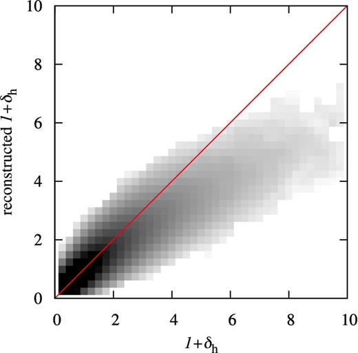
Comparison of the densities of original and reconstructed halo fields in the Millennium simulation for haloes with m < 1011.5 h−1 M⊙. The reconstruction used a grid of size G = 2.5 h−1 Mpc. The halo overdensities δh have been estimated in cubical cells of 53 h−3 Mpc3. The line shows the case where original and reconstructed halo densities are equal.
To test the accuracy of the method, we perform the reconstruction on the MultiDark simulation, which gives us a better probe of the large-scale halo clustering. We measure the halo bias in the low-mass regime from the reconstructed halo catalogue. The halo bias has been estimated by first measuring the halo power spectrum P(k) and then taking the square root of the ratio between the halo power spectrum and that of mass. In this, we assumed the non-linear mass power spectrum given by CosmicEmu (Lawrence et al. 2010).
The recovered halo biases in mass bins below the resolution limit are shown in Fig. 3, which compares the results of using different estimates of the halo density field as well as different biasing models. In this figure, the measured halo bias is shown as a function of the wavenumber for the three mass bins: 1010 < m < 1010.5, 1010.5 < m < 1011 and 1011 < m < 1011.5 h−1 M⊙. We find that the DT method as implemented in the dtfe code (Cautun & van de Weygaert 2011) provides better results than the grid-based estimator with CIC and NGP assignment schemes. The large-scale bias, expected to asymptote to linear theory predictions, is in very good agreement with the predictions of Tinker et al. (2010) in the case of DT, whereas for the other methods the bias is clearly overestimated. This is particularly true in the case of NGP. The DT method better accounts for local variations in number density, reducing the shot noise in the reconstruction and giving a better sampling of the most extreme environments. In the NGP and CIC cases, the significant shot-noise contributions translate into additional scale-dependent components in the power spectrum and estimated bias. In this exercise, we pushed the methods towards their limits by considering a very small grid size of 2.5 h−1 Mpc. However, if we increase the grid size to 5-10 h− 1 Mpc, the recovered halo biases come to agreement and we find that the three methods converge to the same values.

Top: scale-dependent bias of the reconstructed haloes obtained using different methods applied to the MultiDark data to estimate a continuous halo density field. For each of the methods: DT (dotted), CIC (dashed) and NGP (dot–dashed), the three curves correspond to samples of haloes with mass in the ranges 1010 < m < 1010.5, 1010.5 < m < 1011 and 1011 < m < 1011.5 h−1 M⊙, respectively, from top to bottom, reconstructed using the haloes above the upper mass limit in each case. Bottom: scale-dependent bias of the reconstructed haloes obtained using linear and power-law bias prescriptions in the reconstruction. In these cases, the DT method has been used to estimate a continuous halo density field. In all panels, the horizontal lines are the linear halo bias predictions by Tinker et al. (2010) for the three mass bins considered.
The biasing scheme that enters in the conditional mass function has also some impact on the recovered halo clustering, in particular for small-grid-size density field reconstruction such as the one considered here. We show in the bottom panel of Fig. 3 the effect on the recovered halo bias when assuming a linear or power-law bias model as described in Section 2.2. In both cases, we use the halo density field reconstructed with the DT method. We find that the linear model tends to overestimate the large-scale linear bias for low-mass haloes compared to the power-law model, which instead allows us to recover the linear bias predictions of Tinker et al. (2010) at the few per cent level.
It is noticeable in Fig. 3 that, as is inevitable, one cannot reconstruct the highest k regime of the halo power spectrum. This however does not really matter for the purpose of galaxy mock construction, since the overall galaxy power spectrum is dominated by the 1-halo term in this regime, as we will show in the next section.
Another aspect which can be important for creating realistic halo catalogues is the assignment of velocities to the newly created haloes. Their velocity should sample the underlying velocity field which can be estimated from the original haloes. The velocity field is a volume-weighted quantity and for this reason it is more difficult to measure than the density field from the set of original haloes. It has been shown that the DT method is particularly efficient at recovering the velocity field, and it naturally avoids the velocity field to be artificially set to zero in regions where there are no haloes, which can be the case for mass-weighted approaches based for instance on interpolating the velocities to a grid (e.g. Jennings 2012). The estimated velocity field with DT can thus be used and interpolated at the position of the reconstructed haloes so that reliable velocities can be assigned to them.
4 APPLICATION TO GALAXY MOCK SAMPLE CONSTRUCTION
The reconstruction of the halo density field below the resolution limit in cosmological simulations is particularly useful in the context of building realistic galaxy mock surveys. As explained earlier, forthcoming large cosmological surveys of galaxies will need a large number of mock survey realizations, and we need these mocks to include galaxies of very low luminosity/stellar mass. These dim galaxies sit in low-mass haloes, so that a method such as the present one is required to restore such missing haloes. In the following, we apply our halo reconstruction method and test its efficiency in this context.
An efficient way to build galaxy mock samples is to use the HOD formalism (Peacock & Smith 2000; Seljak 2000; Cooray & Sheth 2002), which enables us to populate haloes with galaxies in a way that accurately reproduces the galaxy clustering. We use this technique on the Millennium simulation to build galaxy catalogues mimicking Sloan Digital Sky Survey DR7 (SDSS; Abazajian et al. 2009) volume-limited samples at z ≃ 0.1. We create two absolute magnitude-selected samples corresponding to Mr − 5 log (h) < −18 and Mr − 5 log (h) < −19 from the halo occupation measurements performed by Zehavi et al. (2011). We choose these cuts because they involve a significant fraction of the galaxies residing in the low-mass end of the halo mass function. In practice to create the galaxy catalogues, we populate haloes with central and satellite galaxies using the mean occupation numbers given by the HOD. While central galaxies are placed at halo centres, satellite galaxies are randomly disposed around halo centres in such a way that their radial distribution follows an NFW (Navarro, Frenk & White 1996) density profile. The details of the procedure are given in appendix B of de la Torre & Guzzo (2012). For each volume-limited sample, we construct three catalogues: one based on the original complete halo catalogue to which we refer in the following as the fiducial sample, a second built from a reconstructed halo catalogue below mlim = 1011.5 h−1 M⊙ using G = 2.5 h−1 Mpc and a third one built from a reconstructed halo catalogue below mlim = 1011 h−1 M⊙ using G = 1 h−1 Mpc. In these reconstructions, we estimated the halo density field using the DT method and assumed the power-law bias model in the conditional mass function.
We present in Fig. 4, the galaxy two-point correlation functions for the two absolute magnitude-selected mock samples built from the original complete halo catalogue. These are compared to those measured in the mock samples in which the haloes of masses below mlim = 1011.5 and 1011 h−1 M⊙ have been reconstructed. In the case of the reconstruction with mlim = 1011.5 h−1 M⊙ and G = 2.5 h−1 Mpc, we find that the correlation functions obtained are well recovered, although the correlation function is underestimated by up to 15 per cent on intermediate scales for the Mr − 5 log (h) < −18 sample. This underestimation is a direct consequence of the resolution scale chosen for the reconstruction. Indeed, the clustering drops on smaller scales than the reconstruction scale for the reconstructed low-mass haloes. This in turn causes the observed underestimation of the correlation function of less luminous galaxies. However, by reconstructing the halo density field on smaller scales, i.e. by using a lower mass limit for the reconstruction of mlim = 1011 h−1 M⊙, one can better reproduce the halo clustering on 1 h−1 Mpc scales and eliminate the underestimation as shown in Fig. 4. The differences seen are lower than 1 per cent, below the impact of the simplifying assumption of spherical haloes used in the HOD approach (van Daalen, Angulo & White 2012). We note that the small-scale galaxy clustering, i.e. below 0.7−1 h−1 Mpc, is always well recovered. This comes from the fact that the galaxy distribution inside haloes is independent of the halo clustering by construction (de la Torre & Guzzo 2012) and the clustering on those scales is dominated by this 1-halo term.

Top panel: comparison of the two-point correlation functions of mock galaxies with Mr − 5 log (h) < −18 (thin lines) and Mr − 5 log (h) < −19 (thick lines) obtained from the original halo catalogue (referred as fiducial in the caption) with those obtained after reconstruction of haloes below 1011.5 h−1 M⊙ (dot–dashed lines) and 1011 h−1 M⊙ (solid lines) in the Millennium simulation. The two reconstructions have been performed, respectively, on grid sizes of G = 2.5 and 1 h−1 Mpc. The amplitude of the correlation functions for the Mr − 5 log (h) < −18 samples has been divided by 5 to improve the clarity of the figure. Bottom panel: relative difference of two-point correlation functions of samples with reconstructed haloes with respect to that of fiducial samples. In the two panels the dotted and solid curves are not distinguishable as they almost overlap completely.
One could improve the method in the case of relatively coarse grid reconstructions by working at the subgrid level and using additional constraints from the mass non-linear power spectrum. Indeed, one could envisage distributing haloes in each subcell so as to reproduce the non-linear correlation function predicted from theory, instead of randomly distributing them. We plan to investigate this extension of the method elsewhere.
5 SUMMARY AND CONCLUSIONS
We have described in this paper a method for populating dark matter simulations with haloes of mass below the resolution limit. It is based on estimating a continuous halo density field and then sampling this stochastically in order to obtain low-mass haloes with the correct abundance and bias. This latter part requires the conditional halo mass function, which is extrapolated from the simulation itself or taken from theoretical predictions.
We found that the method works well and allows us to reproduce the halo distribution below the resolution limit with high fidelity, in particular for reconstructions on grids of size G = 1 h−1 Mpc or below. Moreover, the method is particularly efficient at producing galaxy mock samples from low-resolution simulation halo catalogues. We built galaxy mock samples using the HOD technique on the reconstructed halo density field, tuned to mimic SDSS observations. We showed that within a reasonable resolution limit range, one can recover the overall two-point correlation function at the per cent level.
The method presented here is relatively general. Another possible application is the reconstruction of dark matter distributions. As with the galaxy mock sample construction, one can make use of the halo model to distribute dark matter inside the haloes. Such data sets could then be used to create cosmic shear catalogues from ray tracing through the simulation or to predict the galaxy-lensing signal, a quantity directly related to the galaxy-mass correlation function. Other applications can readily be envisaged – although we caution that they should all be subject to the kind of validation tests that we have performed here.
For the present, this validation has only been performed at the two-point level; however, with this restriction our results demonstrate that one can communicate efficiently the full information content of a large simulation by using only a catalogue of the more massive haloes. This method should be very useful in the future in building realistic galaxy mocks for the massive forthcoming cosmological surveys such as Euclid (Laureijs et al. 2011), where the volume and mass resolution requirements for the survey simulations are both very high.
We thank Gabriella De Lucia for giving us useful comments on the manuscript. The MultiDark Database used in this paper and the web application providing online access to it were constructed as part of the activities of the German Astrophysical Virtual Observatory as result of a collaboration between the Leibniz-Institute for Astrophysics Potsdam (AIP) and the Spanish MultiDark Consolider Project CSD2009-00064. The Bolshoi and MultiDark simulations were run on the NASA's Pleiades supercomputer at the NASA Ames Research Center.
Scottish Universities Physics Alliance.
