


Abstract
We investigate the onset of pressure-driven toroidal-mode instabilities in accretion mounds on neutron stars by 3D magnetohydrodynamic (MHD) simulations using the pluto MHD code. Our results confirm that for mounds beyond a threshold mass, instabilities form finger-like channels at the periphery, resulting in mass-loss from the magnetically confined mound. Ring-like mounds with hollow interior show the instabilities at the inner edge as well. We perform the simulations for mounds of different sizes to investigate the effect of the mound mass on the growth rate of the instabilities. We also investigate the effect of such instabilities on observables such as cyclotron resonant scattering features and timing properties of such systems.
1 INTRODUCTION
Neutron stars in binary systems accrete matter either from stellar winds (Davidson & Ostriker 1973) or from Roche lobe overflow (Ghosh, Pethick & Lamb 1977; Koldoba et al. 2002; Romanova et al. 2003) of the companion. The matter is channelled by the magnetic field to the poles, forming accretion mounds. Radiation from such mounds and the overlying columns gives rise to the pulsating X-ray emission observed due to the rotation of the neutron star (e.g. see Patruno & Watts 2013 and Caballero & Wilms 2012 for some examples of accretion-powered X-ray pulsars).
The pressure of the confined accreted matter distorts the local magnetic field (Hameury et al. 1983; Melatos & Phinney 2001; Payne & Melatos 2004; Mukherjee & Bhattacharya 2012) with important consequences for the X-ray emission from the mounds and secular evolution of the neutron star's magnetic field. For high-mass X-ray binary systems (hereafter HMXB) with companion masses ≃ 5–10 M⊙, the accreted matter confined within a polar cap of radius ∼1 km generates strong broad-band X-ray emission with characteristic cyclotron resonance scattering features (hereafter CRSF; see Coburn et al. 2002; Heindl et al. 2004 for a review). Superposition of spectra from different parts of the mound with strong local distortions in the field lines would tend to make the CRSF structure broad and complex (Mukherjee & Bhattacharya 2012, hereafter MB12). The observed broadening of CRSF at lower luminosity, e.g. in V0332+53 (Tsygankov, Lutovinov & Serber 2010), may be due to larger field distortions closer to the mound.
Over long term, the accreted matter would eventually flow horizontally along the neutron star surface. It has been proposed by various authors (Romani 1990; Young & Chanmugam 1995; Cumming, Zweibel & Bildsten 2001; Melatos & Phinney 2001; Payne & Melatos 2004) that such material flow may drag the field and bury it, leading to the relatively lower fields (∼108–109 G) of neutron stars in low-mass X-ray binaries (hereafter LMXB)1 as compared to the ∼1012 G fields in younger HMXB systems. However, plasma instabilities may disrupt such a burial processes by enabling cross-field transport of matter. Gravity-driven modes may be triggered inside the accretion mound (Cumming et al. 2001) resulting in the formation of closed disconnected loops (Payne & Melatos 2004; MB12; Mukherjee, Bhattacharya & Mignone 2013). Such mounds are also prone to pressure-driven instabilities (Litwin, Brown & Rosner 2001), as is common in systems like tokamaks where highly curved magnetic fields confine internal plasma (see Freidberg 1982 for a review of MHD instabilities in such systems).
In this work, we explore the MHD instabilities in accretion mounds strictly contained inside a polar cap of radius ∼1 km on a neutron star of surface field ∼1012 G. This is appropriate for accretion mounds formed on HMXB and young LMXB with high magnetic field. The effects of gravity-driven modes in such systems have been explored in Mukherjee et al. (2013, hereafter MBM13) via 2D axisymmetric simulations. In this paper, we extend the work of MB12 and MBM13 to perform perturbation analysis in full 3D setting via MHD simulations.
This paper is organized as follows: (i) in Section 2, we describe the equations solved to obtain the equilibrium structure of the mound which is subsequently perturbed and evolved to perform the MHD simulations, (ii) in Section 3, we describe the results of the simulations for mounds of different sizes and structure. We show that higher mass mounds with large field distortions are highly unstable whereas mounds of smaller mass have slower growth rates tending to a stability threshold iii) in Section 4, we discuss the implications of the MHD instabilities on (a) the long-term field evolution in such systems, (b) the spectra and CRSF from mounds on HMXB systems and (c) the timing features expected from such mounds.
2 NUMERICAL SETUP
The equilibrium solutions from the GS solver are used as initial conditions in the pluto MHD code (Mignone et al. 2007). The pluto code solves the full set of ideal MHD equations following the Godunov scheme (e.g. MBM13; Mignone et al. 2007). As the density falls off to zero beyond the mound height, we choose a section of the GS solution as the pluto domain (as in MBM13), such that local Alfvén speeds are non-relativistic. The 2D axisymmetric GS solutions carried out over a polar plane (r-z) are rotated in the azimuthal direction to construct the 3D mound in force equilibrium. The GS solutions are then imported into pluto by a trilinear interpolation scheme. The simulation is carried out in [0, π/2] domain in the azimuthal direction with periodic boundary condition at both ends. Although this does impose an assumed symmetry of a quarter of a quadrant, the results are qualitatively similar to that of a full azimuthal domain [0, 2π], as discussed in Section 3.1.
To minimize numerical errors, the grid spacing was chosen such that the grids are nearly cubic at the centre of the pluto domain (rcΔθ ≃ Δr ≃ Δz, where rc is midway between the radial extremes of the pluto domain). The runs were performed with different grid resolutions to check for the convergence of the solutions (see Section 3.1 for details on comparisons of resolutions). It was found that choosing spatial resolutions less than a metre was sufficient to follow the growth of the instabilities and their subsequent effects (see Table 1 for some typical resolutions used).
Sample resolutions for simulation runs.
| Zc | Nr × Nθ × Nz | Δl (Δr ≃ rcΔθ ≃ Δz) |
|---|---|---|
| Solid mound | ||
| 70 m | 1024 × 1536 × 96 | ∼0.59 m |
| 50 m | 744 × 1168 × 48 | ∼0.67 m |
| 45 m | 824 × 1512 × 48 | ∼0.55 m |
| Hollow mound | ||
| 45 m | 572 × 2096 × 64 | ∼0.52 m |
| Zc | Nr × Nθ × Nz | Δl (Δr ≃ rcΔθ ≃ Δz) |
|---|---|---|
| Solid mound | ||
| 70 m | 1024 × 1536 × 96 | ∼0.59 m |
| 50 m | 744 × 1168 × 48 | ∼0.67 m |
| 45 m | 824 × 1512 × 48 | ∼0.55 m |
| Hollow mound | ||
| 45 m | 572 × 2096 × 64 | ∼0.52 m |
Normalized density and magnetic field (see Table 2 for normalization constants) are interpolated from the GS solutions. Pressure is evaluated from equation (2). The initial velocities and toroidal field are set to zero. For our simulations, we have used the HLL Riemann solver (Toro 2008), a third-order Runge–Kutta scheme for time evolution and a third-order piece-wise parabolic method (PPM) for interpolation (as in Colella & Woodward 1984). For preserving the |$\nabla \cdot \boldsymbol {B}=0$| constraint, we use the extended generalized Lagrange multiplier scheme (e.g. Dedner et al. 2002; Mignone & Tzeferacos 2010; Mignone, Tzeferacos & Bodo 2010) as it gives improved numerical stability. See MBM13 for more discussion on the relevant schemes which are suitable for the problem undertaken.
At the base of the mound (z = 0), we apply a fixed boundary condition to represent a hard crust. At the top and the sides, we apply a fixed gradient boundary condition, where the gradients of the physical parameters are kept fixed to the initial value. This preserves the force equilibrium at the domain boundaries, preventing any artificial gradients that may lead to numerical errors. Such a boundary condition signifies an outflow on the perturbed quantities (see MBM13).
Normalization constants for a simulation with GS solution of a mound with polar field Bp = 1012 G.
| Parameters | Values |
|---|---|
| Magnetic field (Bp) | 1012 G |
| Density (ρ0) | 106 g cm−3 |
| Length (L0) | 105 cm |
| Velocity (|$V_{{\rm A}0} = B_{\rm p}/\sqrt{4 \pi \rho _0}$|) | 2.82 × 108 cm s−1 |
| Time (tA = L0/VA0) | 3.55 × 10⁻⁴ s |
| Parameters | Values |
|---|---|
| Magnetic field (Bp) | 1012 G |
| Density (ρ0) | 106 g cm−3 |
| Length (L0) | 105 cm |
| Velocity (|$V_{{\rm A}0} = B_{\rm p}/\sqrt{4 \pi \rho _0}$|) | 2.82 × 108 cm s−1 |
| Time (tA = L0/VA0) | 3.55 × 10⁻⁴ s |
The equilibrium GS solution is first evolved in pluto without any added perturbation to test the stability of the numerical schemes. For the set of schemes used, the equilibrium solution remains intact without any substantial internal flows. The maximum internal flow velocities at t ∼ 2tA for a 70 m mound with resolution 512 × 768 × 48 is less than 1 per cent of local Alfvén and magnetosonic velocities.
![A horizontal section at z ∼ 25 m of a mound of height ∼70 m, showing the initial normalized random velocity field (see Table 2 for normalization constants). The white lines denote the radial edges of the pluto domain in a cylindrical coordinate system (r, θ, z). The simulation is set up for azimuthal range [0, π/2].](https://oup.silverchair-cdn.com/oup/backfile/Content_public/Journal/mnras/435/1/10.1093/mnras/stt1344/2/m_stt1344fig1.jpeg?Expires=1750477811&Signature=WV~YhWfPEwqbZAnNc7QTmDAnQ7bXq0rjLrj576zPS8Rn5ymcryKfFriyHtrulFDFObfRa-2cQh-UwGCK5b52K~c1X6IAUThE8TAioZN4Mx6nae3lU07f0aREvqj4uTMdPUf3zfT5lavsRnaV3MS7K-GYqlnnWWaMjxzBOkRrfveMLpimT30WMExjtCR1EUkJx5~rvXnYxKmvgl6EKOLoeSctZ~5WWMvNFviFOY6hYBfK9mOZyittzeclc8OhFJzRN~ukZFgRfKQguno5lcJ9tYQGVzWLguajEkMwadXEWRhX6Jg8E-xZxdE-IflylaE03gdZjQCv-SDYseSqTUI85Q__&Key-Pair-Id=APKAIE5G5CRDK6RD3PGA)
A horizontal section at z ∼ 25 m of a mound of height ∼70 m, showing the initial normalized random velocity field (see Table 2 for normalization constants). The white lines denote the radial edges of the pluto domain in a cylindrical coordinate system (r, θ, z). The simulation is set up for azimuthal range [0, π/2].
3 RESULTS
3.1 Toroidal-mode instabilities in filled mounds
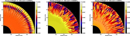
Density normalized to equilibrium value showing the development of the MHD instabilities at different times. At the onset of the instabilities radial fingers of overdense structures are formed due to development of toroidal modes. With time the radial fingers merge and spread throughout the mound.
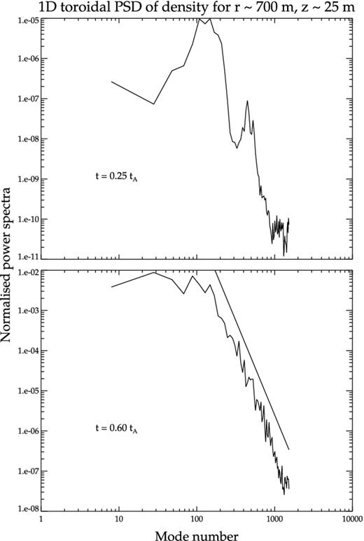
1D PSD at r ∼ 700 m and z ∼ 25 m at times t ∼ 0.2tA and ∼ 0.6tA, respectively (corresponding to the first two panels in Fig. 2). The x-axis gives the mode number (see the text). A line is drawn parallel to the PSD in the second plot to show the power-law nature of the Fourier spectra.
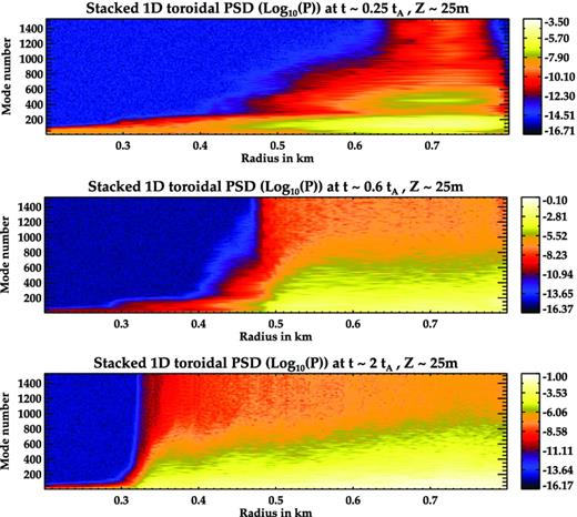
Stacked 1D PSD of perturbed density at different radii and times (corresponding to the panels in Fig. 2). At the initial stages of the development of the instabilities (t ∼ 0.25tA), power is concentrated in some distinct modes. At later times, power is spread over all scales. The instability is seen to spread inwards as there is increase in power at the inner radii with time.
The final form of the density distribution is shown in Fig. 5. Finger-like streams are clearly seen to extend throughout the mound. The magnetic field also develops finger-like channels across the azimuthal domain with alternate regions of high and low field, which are complementary to the density streams (see Fig. 6). Structures of higher density settle in valleys between the magnetic channels as matter tries to flow out radially. Although poloidal field is dominant, there is a substantial build-up of toroidal fields from an initial zero value. As seen in Fig. 6, the toroidal field is intermittent with alternate strips of negative and positive regions signifying local eddies and churning of internal fields.
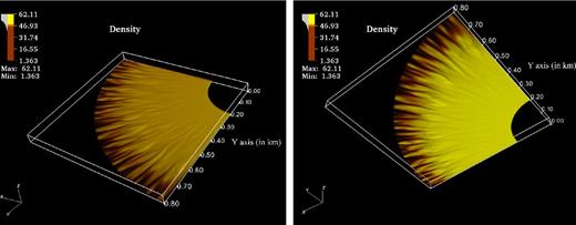
The top (left figure) and bottom (right figure) view of 3D density contours at t ∼ 2tA for Zc = 70 m filled mound with Bp = 1012 G. The density is in the units of 106 g cm−3. The finger-like channels are clearly seen at the outer edge.
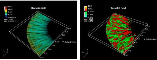
Left: 3D contours of magnetic field magnitude at t ∼ 2tA for Zc = 70 m filled mound with Bp = 1012 G. The field values are in units of 1012 G. Alternate channels are clearly seen to form magnetic valleys which coincide with density streams in Fig. 5. Right: 3D contours of Bϕ showing alternate strips of positive and negative toroidal components signifying turbulent eddies.
Energy. The total energy of the mound is dominated by its internal and gravitational potential energy components, magnetic energy contributing only a small fraction (∼5.5 per cent of internal energy at t = 0). The various energy components remain almost constant with very little change till the instability onset time2tinst ∼ 0.3tA (see Fig. 7), beyond which the rate of change of the energy components increases due to the onset of MHD instabilities. This also corresponds to the time when the finger-like radial channels are formed throughout the mound. Thus, for the ∼70 m mound, the instabilities start acting after ∼ 0.3tA. The internal and gravitational energy decrease as some part is converted to magnetic energy and the rest is lost through outflows from the periphery. The system is dominated by poloidal field components. Although toroidal fields are generated due to internal motions, they contribute only a maximum of 2.3 per cent of the total magnetic energy. As the instabilities saturate, stretching and twisting of field lines increases the magnetic energy (∼20 per cent increase at t ∼ 2tA).
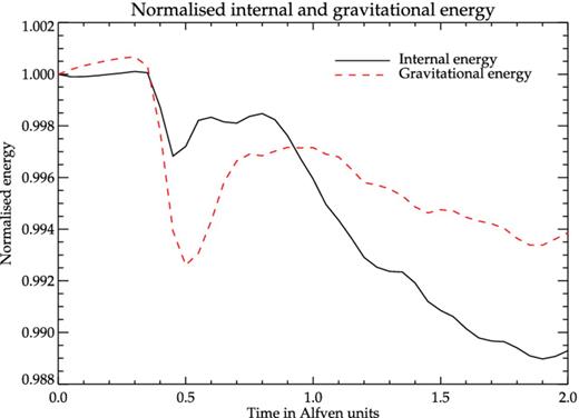
Internal and gravitational potential energy normalized to their initial values ∼2.76 × 10²³ and ∼3.21 × 10²³ erg, respectively.
2π versus π/2 in azimuthal domain. As the runs were computationally expensive, we have performed most of the simulation over a quadrant of the azimuthal domain. This assumes periodic boundary conditions at θ = 0 and θ = π/2. Such an approximation does restrict some large m modes from growing. However, if the dynamics is dominated by local variations in physical parameters, then short-wavelength modes are expected to dominate. To test the validity of our results, we have performed a few simulations for the full azimuthal domain [0, 2π] for a smaller evolution time and compared them with single quadrant simulations. The results are qualitatively similar in both cases with similar nature of the growth of the instabilities (see Fig. 8 for normalized density at ∼ 1tA). It is seen that the PSD of the physical parameters (e.g. density) at different heights and radii are very similar for both cases (see Fig. 9 for a comparison at t ∼ 0.25tA), indicating that the results of our simulations are not significantly affected by constraining the domain to [0, π/2]. Hence, further runs have been performed over the [0, π/2] domain of the azimuthal angle.
![Density of a 70 m mound at z ∼ 25 m, normalized to equilibrium value, for a simulation run with azimuthal domain: [0, 2π]. The entire mound develops alternating density channels in the azimuthal direction destroying the axisymmetry of the equilibrium solution.](https://oup.silverchair-cdn.com/oup/backfile/Content_public/Journal/mnras/435/1/10.1093/mnras/stt1344/2/m_stt1344fig8.jpeg?Expires=1750477811&Signature=StK3hrZouoCLQKV3rAs-YRe3ZGlcAy-tPaP9Rj~P0hn-cB9yFcURvGXBJvKVyOO3ZmtOAdbAHlAR~~BWhamY6xiuDVoT9pUtYIJKW2M5J610TlzJsU7Z5i4VkP5tenQN6g-JxhL0r7OL1vbIFeaBAMYr8dtQig9~bn6Pusm7TzyTwo7lBoN8pw9K-nNIyU~BYlpGrQW7MpeOsCVLayAws7R-s4XxCvPjbICPfqKZvzChhqtGohDx9gfRwaRaRjCgFfLXqheRPXUIPjLfxGNEXsE9qcnfJtPaDzVsbdE6vjVpmK43ThUb7OClT2GO-R25PYuVAFojbtAsKSZObIGMpg__&Key-Pair-Id=APKAIE5G5CRDK6RD3PGA)
Density of a 70 m mound at z ∼ 25 m, normalized to equilibrium value, for a simulation run with azimuthal domain: [0, 2π]. The entire mound develops alternating density channels in the azimuthal direction destroying the axisymmetry of the equilibrium solution.
![PSD of 1D fast Fourier transform (FFT) of perturbed density at r ∼ 700 m, z ∼ 25 m and t ∼ 0.25tA for simulation runs with azimuthal domains [0, 2π] (in black) and [0, π/2] (in red). The PSD of the two runs closely resemble each other confirming that growth of MHD instabilities is qualitatively similar in both cases.](https://oup.silverchair-cdn.com/oup/backfile/Content_public/Journal/mnras/435/1/10.1093/mnras/stt1344/2/m_stt1344fig9.jpeg?Expires=1750477811&Signature=msJ05tGDE-bsOvfZyAALpe3ZShhn-HssZyWA30o69T7f1qYYTbtPwm6ywKNSVdxScAD4YYqDK1pJbSdswSjPqt0mS07JKG2nRltYi4yq1NeNo~EzYDC1Yjv~SscKUiBacfUtVhcUQw~3~i8NbMP~2btjoS6eaPe6zgOTKrw-qK-1TJJzU4miZjvj1XXhUfrAByeSNusPj5Yh8qZPxy4IYcYXWBwLrE8vmvqiWgPK0wtE6uZjC700wzLDp682uVztkxVFPphAT7rZOLiCviAplmd1vGWWfSMBdTVk6uW-D0EbTplpqveBS352rXFgGL~s0WqDmMHewc7q53uI~wswCQ__&Key-Pair-Id=APKAIE5G5CRDK6RD3PGA)
PSD of 1D fast Fourier transform (FFT) of perturbed density at r ∼ 700 m, z ∼ 25 m and t ∼ 0.25tA for simulation runs with azimuthal domains [0, 2π] (in black) and [0, π/2] (in red). The PSD of the two runs closely resemble each other confirming that growth of MHD instabilities is qualitatively similar in both cases.
Resolution dependence. We have performed the simulation at different resolutions to check for convergence. At higher resolutions more internal structures are resolved. As cross-field diffusion is reduced, field lines are deformed at earlier times due to internal flows.3 Thus, higher resolutions result in faster onset of the instabilities, which has also been demonstrated for 2D simulations in MBM13. However, we have found that for grids with spatial resolutions ≤1 m, the results of the MHD instabilities are qualitatively similar. In Fig. 10, the density at t ∼ 0.75tA and z ∼ 25 m is plotted for three different resolutions (Nr × Nθ × Nz): 256 × 384 × 24, 512 × 768 × 48 and 1024 × 1536 × 96, respectively. It is seen that for the simulation with radial grid size Nr = 256 the radial structures have not developed yet, whereas for the simulations with Nr = 512 and 1024, the toroidal modes have fully developed and reached the non-linear saturation phase. The time evolution of the gravitational potential energy at different resolutions are compared in Fig. 11 (other energy components behave similarly). There is a tendency for the energy curves to converge at higher resolution. It can be seen that the runs with Nr = 512 and 1024 resemble each other better than that with Nr = 256. Thus, further simulations were performed with the resolution set to 512 × 768 × 48, which corresponds to a spatial resolution of ∼1 m at the centre of the domain. Similar resolution settings have been adopted for mounds of different sizes.
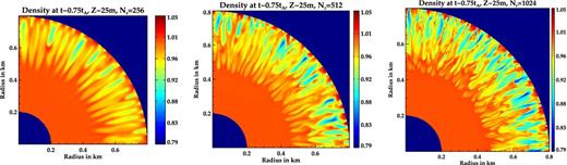
Density normalized to equilibrium value at t ∼ 0.75tA and z ∼ 25 m for different resolutions (Nr × Nθ × Nz): 256 × 384 × 24, 512 × 768 × 48 and 1024 × 1536 × 96, respectively.
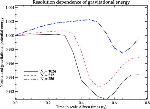
Evolution of gravitational potential energy for three different resolutions (as in Fig. 10) with number of radial cells as: Nr = 256, 512 and 1024. See the text for details.
3.2 Mounds of medium size: threshold of stability
Mounds of smaller mass with less field distortion display slower growth of instabilities. For mounds near the GS threshold (e.g. Zc ∼ 70 and 65 m), the instability onset time is tinst ∼ 0.3tA and ∼ 3.5tA, respectively, whereas for smaller mounds it is larger, e.g. tinst ∼ 1.1tA for Zc = 55 m and ∼ 2.5tA for Zc = 50 m (see Fig. 12). For a 50 m mound, the density initially settles in stationary pockets of lower field strength (see Fig. 13). The initially formed filaments remain stationary till ∼ 2.5tA after which the instability starts to spread throughout the mound with a corresponding change in the energy components (see Fig. 12 for magnetic energy plot).
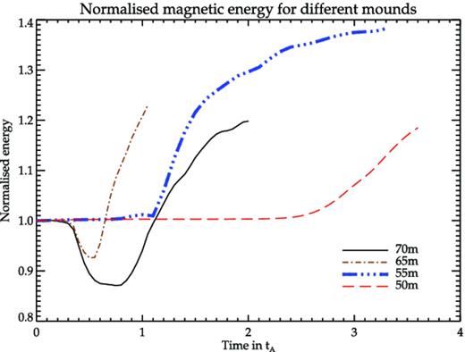
Magnetic field energy for different mound heights. The runs have been evolved till the MHD instabilities have sufficiently developed. The instability onset time tinst (see the text) is greater for larger mounds.
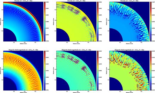
Top: density normalized to equilibrium value at z ∼ 10 m at different times. Bottom: magnetic field magnitude normalized to equilibrium value at z ∼ 10 m. At the initial phases the density settles in stationary pockets of low-field regions, which starts to spread at later times.
For a Zc = 45 m mound, MHD instabilities do not grow during the run time of the simulation. The perturbed mound quickly settles into a steady state after some initial oscillations (see Fig. 14). Thus, with decrease in mound mass, the system tends to become stable. This agrees with the results of Litwin et al. (2001) which predict that accretion mounds are unstable only if plasma β = p/(B2/8π) is higher than a threshold value. As shown in the discussion of MBM13, the maximum plasma β for a Zc = 45 m mound is very close to such a threshold. This confirms that filled mounds of central height lower than ∼45 m may be stable with respect to pressure-driven ballooning instabilities.
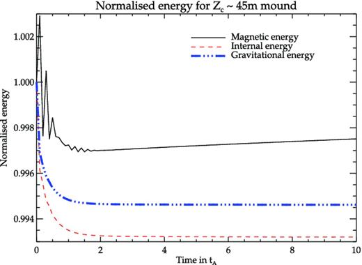
The energy components for Zc = 45 m mound normalized to their initial values: internal energy to ∼5.1 × 10²³ erg, gravitational potential energy to ∼3.3 × 10²³ erg and magnetic energy to ∼8.8 × 10²¹ erg. The internal and gravitational energy relax to a stationary state after a very small change from the initial value. The magnetic energy also settles down after some initial oscillations. The magnetic energy in the steady state is seen to have a slight increasing trend over ∼ 10tA, but the change is very small (∼0.05 per cent).
3.3 Hollow mound
As discussed in MBM13, a finite range of the mass loading region in the accretion disc will result in the formation of hollow ring-like accretion mounds on the neutron star surface. The GS solutions and results from 2D perturbation tests have already been discussed in MBM13. Here, we perform 3D perturbation tests of GS solutions of such mounds (equation 4 with Zc = 45 m). As in filled mounds, multiple radial streams appear at the outer edge. The instabilities saturate by about ∼ 2tA, as is evident from the flattening of the energy curves after initial changes (see Fig. 15). However, unlike in filled mounds, radial streams also appear at the inner boundary (see Fig. 16), which is characterized by a second dip in the internal energy at ∼ 5tA. The toroidal-mode instabilities will cause radial outflow of matter at both outer and inner radial edges, which may, in time, fill up the interior of the hollow mound. However, due to constraints of compute resources, we have not been able to evolve the system for long enough to detect significant mass-loss in our current runs. In any case, the restrictive boundary conditions used in our simulations would be unable to provide an adequate description of mass outflow.
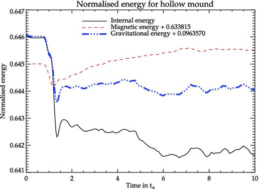
Energy components of a simulation run with hollow mound normalized to E0 = 7.95 × 10²² erg. The magnetic energy is plotted with an offset of ∼0.096E0 and gravitational potential energy with an offset of ∼0.63E0 to represent all three components in the same scale. The magnetic energy is seen to increase by ∼5 per cent before reaching a plateau in the non-linear saturation phase.
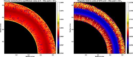
Left: density (normalized to equilibrium value) of a hollow mound at t ∼ 10tA and z ∼ 20 m. The accretion geometry modelled is that of a ring-like mound with hollowed interior. Right: corresponding magnetic field magnitude in units of 1012 G. The finger-like streams throughout the domain show the spread of MHD instabilities at both outer and inner radii of the hollow mound.
4 DISCUSSION
In this paper, we have performed 3D MHD simulations of perturbed accretion mounds which are initially in force equilibrium. We have confirmed the onset of pressure-driven toroidal-mode instabilities. Litwin et al. (2001) had shown that m ≠ 0 non-axisymmetric modes will disrupt the equilibria for mounds beyond a threshold mass. Such ballooning-type instabilities are multidimensional in nature and require a full 3D simulation for their investigation. Our simulations show that such instabilities result in the formation of multiple radially elongated streams distributed in the azimuthal direction. Part of the internal and gravitational potential energy is converted to magnetic energy and the strength is increased by the stretching of field lines due to internal motions. There is a substantial increase in the toroidal magnetic field component (from the initial zero value). The instabilities grow more slowly in mounds of smaller size, and for mounds smaller than a threshold, instabilities were not excited within the run time of the simulations. This roughly corresponds to the threshold discussed by Litwin et al. (2001) e.g. for a Zc = 45 m mound; from our GS solutions we have βmax = 293, which is close to the threshold β (∼260) predicted by Litwin et al. (2001) for MHD instabilities (see discussion in MBM13).
A threshold mound mass was obtained by MB12 from static solutions, which was shown in MBM13 to correspond to the mass threshold beyond which gravity-driven instabilities are triggered. From our current 3D MHD simulations, we predict a lower mass threshold (∼5 × 10⁻¹³ M⊙ for Bp ∼ 1012 G) above which pressure-driven instabilities will start operating and matter will not be efficiently confined by the local field in the polar cap. Further addition of mass will result in the formation of radial density streams nestled in magnetic valleys and matter will flow out of the polar cap to spread over the surface of the neutron star. Our current simulations, limited by computational resources, could not follow the evolution of the mound beyond a few Alfvén times. However, we can expect that with continued accretion, there will be a dynamic equilibrium between inflow from the top and outflow from the sides. Such an outflow, aided by MHD instabilities, may prevent the secular process of field burial often invoked to explain the low magnetic fields of neutron stars in LMXBs and millisecond pulsars.
Semi-analytic work and MHD simulations by Payne & Melatos (2004, hereafter PM04), Payne & Melatos (2007) and Vigelius & Melatos (2008) address the problem of field burial by accretion and come to the conclusion that mounds of size ∼10−4 M⊙ can cause the field to be buried. However, our current work differs from the approach of PM04 in various aspects. We consider the confined matter to be a degenerate Fermi plasma whose pressure is several orders of magnitude larger than that of an isothermal gas considered in PM04. PM04 employ plasma loading on all field lines up to the equator, whereas we confine the plasma strictly within a small polar cap. The excess mass loaded on to the field lines beyond the polar cap in PM04 provides additional lateral support which helps in the formation of large mounds and possible eventual burial of the local field.
In our current work, we have not addressed the burial problem directly, as we have limited ourselves to accretion mounds strictly confined within the polar cap with a fixed boundary far from the surface. Such a situation is more applicable to HMXB or young LMXB systems where higher field strengths and lower accretion rates result in mounds of smaller mass and size. If such a neutron star is to evolve into a low-field object by field burial, the process should commence at this early stage itself. However, our current work hints that pressure-driven instabilities, which have so far been ignored, may play an important role in limiting the efficacy of the burial process. Since our current pluto simulations are limited to a vertical extent less than the mound height, dynamic field distortions above the mound cannot be probed by them. However, from the static GS solutions in Figs 17 and 18, it is clear that although the mound is only a few tens of metres high, the distortions in the field lines last for several hundred metres. This implies that distortions in the mound structure due to the MHD instabilities will also affect the field structure far away from the mound, leaving their imprint on the cyclotron lines (CRSF) from the accretion column.
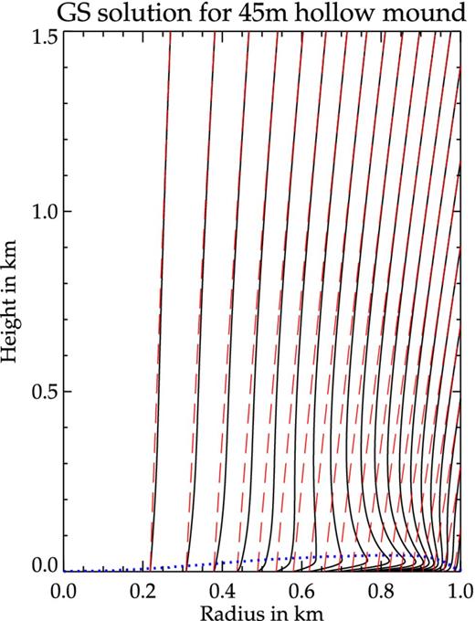
Field lines from the GS solution for a hollow mound (in black) of height ∼45 m and pre-accretion dipolar field (in red). The blue dotted line represents the top of the mound. There is significant distortion in the field from the initial dipole nature for several hundred metres above the mound (∼5 per cent deviation from dipole field at ∼500 m). Far from the neutron star surface (∼1 km and above) the field lines become dipolar.
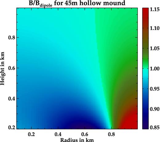
The ratio of BGS to Bdipole for the solution in Fig. 17. The field is plotted for heights ≥200 m to represent the field variation in the column above the mound. Field lines pushed to the periphery cause enhancement of magnetic field at the outer wall of the column and decrease in strength at the inner walls.
Any distortion in the field lines will introduce broadening and complexity in the CRSF structure. To illustrate this, we have evaluated the CRSF by taking the field distribution at the top of the pluto domain at the end of the simulation run ( ∼ 3.6tA) of a Zc = 50 m mound using the method outlined in MB12.4 Fig. 19 shows the effect of broadening of the CRSF due to superposition of spectra from different parts of the mound. The extent of such broadening is expected to increase with accretion rate. MHD instabilities may also produce observable timing signatures from accreting neutron stars. Although any radiation from the mound will be reprocessed in the overlying column, oscillations set up in the mound will be carried higher up in the column by the magnetic field, which will add to the noise observed in the power spectra from these systems. The rapid formation of the density streams within a few Alfvén times and subsequent oscillations in similar time-scales will inject power in the fluctuation spectrum at frequencies corresponding to local instability growth rates. We have calculated the PSD from the Fourier transform of a simulated light curve from the surface of a hollow mound of Zc = 45 m, by assuming the intensity of the local emission to depend on density as I ∝ ρ2 (see Fig. 20). We integrate this over the top of the pluto domain to get the flux as a function of time, for a duration of 10tA = 3.5 × 10− 3 s, corresponding to the longest run amongst the current set of simulations. The light curve clearly shows repetitive patterns which contribute to a broad feature of excess power around ∼800 Hz in the power spectrum. Bumps at kilohertz frequencies corresponding to local Alfvén time-scales are also seen. Thus, MHD instabilities can result in oscillations in the emergent intensity which can show up as broad features in the power spectra of observed X-ray flux and also contribute to high frequency noise.
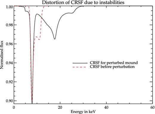
CRSF calculated for the field at the top of a pluto domain for a Zc = 50 m mound. The red line shows the CRSF before the onset of instabilities. Distortion in the field due to instabilities broaden the CRSF. In reality the CRSF profile may be different due to reprocessing of the profile in the accretion column, but there will be a general tendency of broadening of the CRSF with the onset of instabilities.
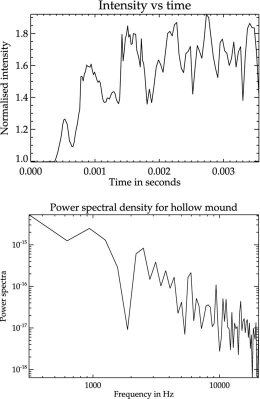
Top: intensity of emission from the top of the mound assuming I ∝ ρ2. Bottom: PSD of the light curve.
Although power spectra of HMXB systems are mostly dominated by low-frequency features arising in the accretion disc, some sources such as Cen X-3 (Jernigan, Klein & Arons 2000) show excess power in the high-frequency regime which has been attributed to instabilities in the accretion column. Some sources show correlation between the photon index and the frequency of the main noise component which indicates that they may originate from the same physical region inside the accretion column (Reig & Nespoli 2013). For mounds of smaller mass, the growth rates being smaller, the characteristic frequencies at which the power would peak due to the MHD processes would also be lower. However, to explore the nature of the power spectra at lower frequencies, longer simulation runs need to be performed.
We thank CSIR India for Junior Research Fellow grant, award no 09/545(0034)/2009-EMR-I. We thank Dr Petros Tzeferacos for his help and suggestions in setting up the boundary conditions in the pluto simulations. We also thank Dr Kandaswamy Subramanian of IUCAA and Dr Biswajit Paul of RRI for useful discussions and suggestions during the work, and IUCAA HPC team for their help in using the IUCAA HPC where most of the numerical computations were carried out. We thank the anonymous referee for his/her kind comments. DB acknowledges the hospitality of ISSI, Berne and discussions with the Magnet collaboration which have benefited this paper.
Companion mass ≤1 M⊙.
Defined here is the time at which the magnitude of the rate of change of the energy components increases by more than a factor of 10 of the initial value.
As we work in the ideal MHD limit, dissipation is numerical in nature and decreases with increase in resolution. In real systems this will be controlled by resistive effects at small scale.
It is to be noted that this exercise may not reproduce realistic CRSF, as the X-ray emission may be further reprocessed in the overlying accretion column.
