


Abstract
We present measurements of higher order clustering of galaxies in the latest release of the Canada–France–Hawaii Telescope Legacy Survey (CFHTLS)-Wide. We construct a series of volume-limited sample of galaxies containing more than one million galaxies over the redshift range 0.2 < z < 1 in the four independent fields of the CFHTLS-Wide. Using a counts-in-cells technique we measure the variance |${\bar{\xi }}_2$| and the hierarchical moments |$S_{n}= {{\bar{\xi }}_n / {\bar{\xi }}_2^{n-1}}$| (3 ≤ n ≤ 5) as a function of redshift and angular scale. We find that the measured field-to-field scatter in our estimators is in excellent agreement with analytical predictions. At small scales, corresponding to the highly non-linear regime, we find tentative evidence at the 1σ level that the hierarchical moments increase with redshift. At large scales, corresponding to the weakly non-linear regime, our measurements are marginally consistent with perturbation theory predictions for standard Λ cold dark matter cosmology using a simple linear bias. The predictions of perturbation theory tend to slightly overestimate our measurements, which may be a signature of non-linear bias.
1 INTRODUCTION
In the current paradigm describing the evolution of the Universe, structures originate from tiny density fluctuations emerging from a primordial Gaussian field after an early inflationary period. Gravitational instability in a homogeneous expanding Universe dominated by cold dark matter (CDM) gives rise to the rich variety of structures seen today by hierarchical clustering. This picture has shown to be consistent with measurements in million-galaxy surveys of the local Universe such as the Sloan Digital Sky Survey (SDSS)1 and 2dF (Colless et al. 2001); however, our knowledge of the evolution of the distribution of galaxies and its changing relationship with underlying dark matter density field remains incomplete.
On small scales, the evolution of the galaxy distribution strongly depends on the physical processes of galaxy formation, while on larger scales, both the initial power spectrum and the global geometry of the Universe play an important role. Precise measurements of the galaxy distribution as a function of redshift and galaxy type therefore represent a fundamental tool in cosmology and the n-point correlation functions provide a particularly powerful method to characterize it.
The two-point correlation function is the one of most widely used statistics (e.g. Peebles 1980; Baumgart & Fry 1991; Martínez 2009, for a general review on the subject) as it provides the most basic measure of galaxy clustering – the excess in the number of pairs of galaxies compared to a random distribution as function of angular scale. However, the two-point correlation function represents a complete description of clustering only in the case of a Gaussian distribution for which all higher order connected moments vanish by definition. It is well known that the actual galaxy distribution is non-Gaussian (e.g. Fry & Peebles 1978; Sharp, Bonometto & Lucchin 1984; Szapudi, Szalay & Boschan 1992; Bouchet et al. 1993; Gaztanaga 1994). This non-Gaussianity is induced by non-linear gravitational amplification of mass fluctuations even if they originated from an initial Gaussian field (e.g. Peebles 1980; Fry 1984; Juszkiewicz, Bouchet & Colombi 1993; Bernardeau et al. 2002, and references therein). It can also be present in the initial conditions themselves, from topological defects such as textures or cosmic strings (Kaiser & Stebbins 1984) or fluctuations coming from certain inflationary models (Guth 1981; Bartolo et al. 2004, and references therein). In addition, the process of galaxy formation results in a ‘biased’ distribution of luminous matter with respect to the underlying dark matter, which adds another level of complexity in the non-Gaussian nature of the process (e.g. Politzer & Wise 1984; Bardeen et al. 1986; Fry & Gaztanaga 1993; Mo & White 1996; Bernardeau et al. 2002, and references therein). For all these reasons, measurements of higher order moments are required to obtain a complete statistical description of the galaxy distribution.
In this paper we will use a counts-in-cells technique to investigate the evolution of the variance |${\bar{\xi }}_2$| and the hierarchical moments |$S_{n}= {{\bar{\xi }}_n / {\bar{\xi }}_2^{n-1}}$| (3 ≤ n ≤ 5) of the galaxy distribution from z ∼ 1 to present day. Until now, the majority of papers which have measured these quantities have analysed large local Universe redshift surveys; see Ross, Brunner & Myers (2006, 2007) for the SDSS and Baugh et al. (2004) and Croton et al. (2004, 2007) for the 2dF Galaxy Redshift Survey (2dFGRS). Furthermore, only a few measurements have been made in the literature of the redshift evolution of the hierarchical moments. For example, Szapudi et al. (2001) used a purely magnitude-limited catalogue of ∼710 000 galaxies with IAB < 24 in a contiguous 4 × 4 deg2 region. By assuming a redshift distribution for their sources, they found that a simple model for the time evolution of the bias was consistent with their measurements of the evolution of S3 as a function of redshift. They concluded that these observations favoured models with Gaussian initial conditions and a small amount of biasing which increases slowly with redshift. Using spectroscopic redshifts from the VIMOS-VLT Deep Survey (VVDS), Marinoni et al. (2008) reconstructed the three-dimensional fluctuation to z ∼ 1.5 and measured the evolution of |$\bar{\xi }_{2}$| and S3 over the redshift range 0.7 < z < 1. They found that the redshift evolution in this interval is consistent with predictions of first- and second-order perturbation theory.
Measuring accurately the higher order moments of the galaxy distribution requires both very large numbers of objects and also a precise control of systematic errors and reliable photometric calibration: no previous surveys have the required combination of depth and areal coverage to make reliable measurements from low redshift to z ∼ 1 in large volume-limited sample of galaxies. In this work, we use will data from the most recent release of the Canada–France–Hawaii Telescope Legacy Survey (CFHTLS) which has a unique combination of depth, area and image quality, in addition to an excellent and highly precise photometric calibration.
The paper is organized as follows. In Section 2, we present our data set and the sample selection. In Section 3, we outline the techniques we use to estimate the galaxy clustering starting from the two-point correlation function and going to higher orders. The results are described and interpreted in Section 4. Conclusions are presented in Section 5.
Throughout the paper we use a flat ΛCDM cosmology (Ωm = 0.27, ΩΛ = 0.73, |$H_{0}= 100\,h \, \rm {km}\, \rm {s}^{-1} \, \rm {Mpc}^{-1}$| and σ8 = 0.8) with h = 0.71. All magnitudes are given in the AB system.
2 OBSERVATIONS, REDUCTIONS AND CATALOGUE PREPARATION
2.1 The Canada–France–Hawaii Telescope Legacy Survey
In this work, we use the seventh and final version of the CFHTLS.2 The T0007 data release results in a major improvement of the absolute and internal photometric calibration of the CFHTLS. Since T0007 is a reprocessing of previous releases, the actual area covered by this release is almost identical to previous versions (some additional observations were added to fill gaps in the survey created by malfunctioning detectors).
The improved photometric calibration has been achieved by applying techniques developed by the Supernova Legacy Survey (Regnault et al. 2009; Betoule et al. 2012) to both the Deep and Wide fields of the CFHTLS. This improved photometric accuracy provides an improved photometric redshift precision and a consistent photometric redshift calibration over the four separate patches of the CFHTLS-Wide.
Complete documentation of the CFHTLS-T0007 release can be found at the3 site. In summary, the CFHTLS-Wide is a five-band survey of intermediate depth. It consists of 171 MegaCam deep pointings (of 1 deg2 each) which, after accounting for overlaps, consists of a total of ∼155 deg2 in four independent contiguous patches, reaching an 80 per cent completeness limit in AB of u* = 25.2, g = 25.5, r = 25.0, i = 24.8, z = 23.9 for point sources. Our photometric catalogues were constructed by running4 in ‘dual-image’ mode on each CFHTLS tile, using the gri images to create a χ2 detection image (see Szalay, Connolly & Szokoly 1999). The final merged catalogue is constructed by keeping objects with the best signal-to-noise ratio from the multiple objects in the overlapping regions. Objects are selected using i-band mag_auto total magnitudes (Kron 1980) and object colours are measured using 3 arcsec aperture magnitudes.
2.2 Photometric redshift and absolute magnitude estimation
The photometric redshifts we used here have been provided as part of the CFHTLS-T0007 release. They are fully documented on the corresponding pages at the5 site and the photometric redshift6 describes in details how the photometric redshifts were computed following (Ilbert et al. 2006; Coupon et al. 2009, 2012).
Photometric redshifts are computed using the7 photometric redshift code which uses a standard template fitting procedure. These templates are redshifted and integrated through the transmission curves. The opacity of the intragalactic medium (IGM) is accounted for and internal extinction can be added as a free parameter to each galaxy. The photometric redshifts are derived by comparing the modelled fluxes and the observed fluxes with a χ2 merit function. In addition, a probability distribution function is associated with each photometric redshift.
The primary template sets used are the four observed spectra (Ell, Sbc, Scd, Irr) from Coleman, Wu & Weedman (1980) complemented with two observed starburst spectral energy distribution (SED) from Kinney et al. (1996). These templates have been optimized using the VVDS deep spectroscopic sample (Le Fèvre et al. 2005). Next, an automatic zero-point calibration has been carried out using spectroscopic redshifts present in W1, W3 and W4 fields. For spectral type later than Sbc, a reddening E(B − V) = 0–0.35 using the Calzetti et al. (2000) extinction law is applied.
Although photometric redshifts were estimated to i < 24, we selected objects brighter than i = 22.5 to limit outliers (see table 3 of Coupon et al. 2009). Star–galaxy separation is carried out using a joint selection taking into account the compactness of the object and the best-fitting templates.
Finally, using the photometric redshift, the associated best-fitting template and the observed apparent magnitude in a given band, one can directly measure the k-correction and the absolute magnitude in any rest-frame band. Since at high redshifts the k-correction depends strongly on the galaxy SED, it is the main source of systematic errors in determining absolute magnitudes. To minimize the k-correction uncertainties, we derive the rest-frame luminosity at a wavelength λ using the object's apparent magnitude closest to λ(1 + z) according to the redshift of the galaxy (the procedure is described in appendix A of Ilbert et al. 2005). For this reason the bluest absolute magnitude selection takes full advantage of the complete observed magnitude set. However, as the u-band flux has potentially larger photometric errors, we use Mg-band magnitudes.
2.3 Sample selection
We select all galaxies with i < 22.5 outside masked regions. At this magnitude, our photometric redshift samples are 100 per cent complete, for all galaxy spectral types. Our photometric redshift errors are small compared to width of our photometric redshift bins.
Here we chose Mg < −20.7 (Mg − 5log h < −19.96) and divide this selection into four redshift bins: 0.2 < z < 0.4, 0.4 < z < 0.6, 0.6 < z < 0.8 and 0.8 < z < 1.0 to construct a volume-limited sample. Our photometric redshift uncertainties are around 5–10 per cent depending on spectral type, and for this reason our samples are necessarily only approximately volume limited. A large bin width (Δz = 0.2) ensures a low bin-to-bin contamination from random errors, but still reduces substantially the mixing of physical scales at a given angular scale that occurs in simple magnitude-selected angular catalogue without redshift information. The redshift distribution of our selection for the four fields is presented in Fig. 1.
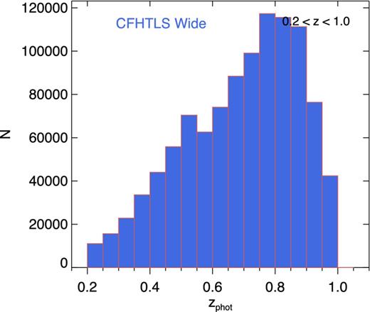
A histogram of the number of galaxies per bin of redshift for all galaxies with Mg < −20.7 in the CFHTLS-Wide T0007 release.
The sample selection is illustrated in Fig. 2. As a means of estimating the approximate completeness of our samples, we measured the mean absolute magnitude |$\bar{M}_{\rm g}$| in each of the redshift bins and found |$\bar{M}_{\rm g} = -21.4\pm 0.1$|. With this selection we have more than 10 000 objects in each bin in each Wide patch. The detailed number of objects in each sample is summarized in Table 1.

A two-dimensional histogram of the number density in the Mg–z plane is plotted for all galaxies in the CFHTLS-Wide, T0007 release. The red line shows our adopted thresholds in absolute luminosity and redshift.
Number of galaxies per redshift bin outside the masked regions.
| W1 | W2 | W3 | W4 | |
|---|---|---|---|---|
| 0.2 < z < 0.4 | 36 307 | 12 121 | 23 426 | 10 945 |
| 0.4 < z < 0.6 | 100 586 | 31 586 | 67 413 | 32 778 |
| 0.6 < z < 0.8 | 165 215 | 48 596 | 105 020 | 59 137 |
| 0.8 < z < 1.0 | 149 960 | 45 783 | 96 737 | 52 423 |
| W1 | W2 | W3 | W4 | |
|---|---|---|---|---|
| 0.2 < z < 0.4 | 36 307 | 12 121 | 23 426 | 10 945 |
| 0.4 < z < 0.6 | 100 586 | 31 586 | 67 413 | 32 778 |
| 0.6 < z < 0.8 | 165 215 | 48 596 | 105 020 | 59 137 |
| 0.8 < z < 1.0 | 149 960 | 45 783 | 96 737 | 52 423 |
3 MEASURING GALAXY CLUSTERING
3.1 Two-point angular correlation function
A random catalogue is generated for each sample with the same geometry as the data catalogue using nr = 106 which is at least six times and at the most 90 times nd for a given bin and patch. We measure w in each field using the site8 in the angular range θ ∈ [0| $_{.}^{\circ}$|001, 1°] divided into 15 bins spaced logarithmically.
In Section 3.4 we explain how the individual measurements of w(θ) from the four different fields are combined.
3.2 Higher order moments
3.3 Measuring counts in cells
The main issue in counts-in-cells measurements is that large scales are dominated by edge effects (Szapudi & Colombi 1996; Colombi, Szapudi & Szalay 1998) due to the fact that, as cells have finite size, galaxies near the survey edges or near a masked region have smaller statistical weights than galaxies away from the edges. To correct for these defects, we use ‘Black Magic Weighted PN’ (BMW-PN; Blaizot et al. 2006; Colombi & Szapudi, in preparation).
This method is based on the fact that counts in cells do not depend significantly on cell shape for a locally Poissonian point distribution. This latter approximation allows one to distort the cells near the edges of the catalogue and near the masks in order to reduce as much as possible edge effects discussed above. In practice, the data and the masks are pixellated on a very fine grid. In this case, one can consider all the possible square cells of all possible sizes. For each of these cells, an effective size is given which corresponds to the area that is contained in the cell after subtraction of the masked pixels. If the fraction of masked pixels in the cell exceeds some threshold f, the cell is discarded. Then, the centre of mass for the unmasked part of the cell is calculated and the algorithm finds the corresponding pixel it falls into. As one cell per pixel is enough to extract all the statistical information, the code selects among all the cells of equal unmasked volume targeting the same pixel the most compact one, i.e. the one which has been the least masked.
Note that the current implementation of BMW-PN works only in the small angle approximation regime. This is not an issue in our analyses as the largest field W1 has an angular extension smaller than 9°.
We used the following parameters in BMW-PN: the sampling grid pixel size was set to 1.93 arcsec, which corresponds to a grid of size 16000 × 13944 for W1. This very high resolution allowed us to probe in detail the tails of the count in cells probability at scales as small as θmin = 0| $_{.}^{\circ}$|0011. We measured counts in square cells of size θ for 15 angular scales, logarithmically spaced in the range θ ∈ [θmin, θmax] with θmax = 1° (see Table B1).
The allowed fraction of masked pixels per cell f is a crucial parameter. If f is too large, the cells become too elongated, invalidating the local Poisson approximation. On other hand, if f is too small, edge effects become prominent. We investigated the following set of values of f for W1 in the redshift bin 0.6 < z < 0.8: f = 0, which corresponds to a traditional counts-in-cells measurement with square cells not overlapping with the edges of the catalogue or the masks, and f = 0.25, 0.5, 0.75. We found that f as large as 0.5 is needed to ensure that edge effects are minimized in the scaling range probed by our measurements. Larger values of f do not change the results significantly so we kept f = 0.5 to reduce as much as possible cell shape anisotropies.
3.4 Combining measurements and errors
Factorial moments (equation 9) are unbiased estimators. However, the quantities we wish to compute, the averaged two-point correlation function |${\bar{\xi }}$| and the hierarchical moments Sn, are non-linear combinations of Fn (equations 7 and 8). For this reason they are themselves biased estimators (e.g. Szapudi, Colombi & Bernardeau 1999).
We use the same weighting procedure as in equation (10) to combine the individual correlation functions wi(θ) measured in each field and derive a combined w(θ). Error bars estimated from the dispersion between our four independent fields are used to estimate statistical uncertainties directly from the data.
Rigorously speaking, a full error propagation formula should be used to compute the statistical uncertainties of w(θ) (Landy & Szalay 1993; Bernstein 1994), |${\bar{\xi }}$| and Sn (Szapudi et al. 1999). However in our case an involved procedure such as this is unnecessary since the uncertainties on the estimated errors themselves are very large as we have only four independent fields. To keep the approach simple while preserving sufficient accuracy we compute the errors on w(θ), |${\bar{\xi }}$| and Sn as for the Fk, by simply replacing Fk, i with wi(θ), |$\bar{\xi }_{i}$| or Sk, i in equation (11) where the quantities |${\bar{\xi }}_{i}$| and Sk, i are derived from Fk, i using equations (7) and (8).
The hierarchical moments and their associated error bars are presented for each redshift bin in Table B1.
Jackknife errors, as advocated by e.g. Norberg et al. (2011) for the SDSS, represent an alternative method to compute errors. As a consistency check, we compared our error estimations with jackknife measurements. To do this we split our four fields into seven patches of approximately the same area (each ∼19 deg2, giving three patches in W1, two in W3 and all of fields W2 and W4). Next, for each ith subfield, we compute the sum of PN(θ) for all fields other than this ith field.9 We used this method to recompute all the quantities of interest for two characteristic redshift bins, 0.4 < z < 0.6 and 0.8 < z < 1.0. We also compare these jackknife measurements to our weighted field-to-field errors using the seven patches of equal size. To do so we derived the quantities calculated on the seven patches and their associated errors bars using equations (10) and (11), finding nearly exactly the same results as for our implementation of the jackknife as in fact expected: one can show that if all the areas of the subfields were exactly the same, both methods would give exactly the same results. At the level of accuracy of our analysis, we found a good agreement between these errors and those derived with our method both for the averaged correlation function and the hierarchical moments in the two redshift bins. Finally, although widely used (e.g. Cabré et al. 2007; Norberg et al. 2009; Zehavi et al. 2011) the jackknife method, in general, is not free of biases because it implicitly neglects long range correlations by assuming that the survey can be decomposed in an ensemble of statistically independent subsamples. Here, we prefer to rely on our unbiased error estimator based on a weighted field to field dispersion. This will be supported by a successful comparison with analytical expectations described below.
3.5 Transformation to physical coordinates
Projection parameters. Columns give the redshift range, scaling distance and n-point amplitude projection factors Fp(n) (equation 23) for n = 3, 4, 5.
| z1 | z2 | x* (Mpc) | Fp(3) | Fp(4) | Fp(5) |
|---|---|---|---|---|---|
| 0.2 | 0.4 | 1280 | 1.09 | 1.28 | 1.61 |
| 0.4 | 0.6 | 1910 | 1.02 | 1.06 | 1.12 |
| 0.6 | 0.8 | 2530 | 1.02 | 1.05 | 1.10 |
| 0.8 | 1.0 | 3010 | 1.09 | 1.25 | 1.46 |
| z1 | z2 | x* (Mpc) | Fp(3) | Fp(4) | Fp(5) |
|---|---|---|---|---|---|
| 0.2 | 0.4 | 1280 | 1.09 | 1.28 | 1.61 |
| 0.4 | 0.6 | 1910 | 1.02 | 1.06 | 1.12 |
| 0.6 | 0.8 | 2530 | 1.02 | 1.05 | 1.10 |
| 0.8 | 1.0 | 3010 | 1.09 | 1.25 | 1.46 |
Finally, in the weakly non-linear regime, it is important to realize that using the hierarchical model to perform the de-projection is strictly not correct, due to the non-trivial angular dependences (Bernardeau 1995). Our comparisons of the measured hierarchical moments with perturbation theory predictions in Section 4.2.4 will take this into account.
3.6 Effect of photometric redshift errors
In order to quantify the effect of the photometric redshift errors on our measurement of Sn, we investigate how important the effect of photometric redshift uncertainty is on the projection factors. To do so we use measurements of photometric redshift uncertainty from Coupon et al. (2009) who compute the photometric redshifts for the CFHTLS-Wide T0004. They use a template-fitting method to compute photometric redshifts calibrated with a large catalogue of 16 983 spectroscopic redshifts from the VVDS-F02, VVDS-F22, DEEP2 and the zCOSMOS surveys. Comparing with spectroscopic redshifts, they find a photometric redshift dispersion in the wide fields of 0.037–0.039 and at i′ < 22.5. Using this dispersion Δz = 0.038 (1 + z) as an estimate of our expected photometric redshift errors, we calculate the average over 20 random redshifts Gaussian distributed around a given photometric redshift zi with a dispersion Δz = 0.038 (1 + zi). These were used to create our new redshift distributions. We note that in general, our photometric redshift errors are smaller than the size of our redshift slices. We derive the numbers presented in Table 3 for x*, Fp(3), Fp(4) and Fp(5).
Projection parameters obtained using photometric redshifts and the dispersion in the estimated redshift of Δz = 0.038 (1 + z). We list the redshift interval, scaling distance and n-point amplitude projection factors Fp(n) (equation 23) for n = 3, 4, 5.
| z1 | z2 | x* (Mpc) | Fp(3) | Fp(4) | Fp(5) |
|---|---|---|---|---|---|
| 0.2 | 0.4 | 1272 | 1.09 | 1.29 | 1.64 |
| 0.4 | 0.6 | 1905 | 1.02 | 1.07 | 1.14 |
| 0.6 | 0.8 | 2530 | 1.02 | 1.06 | 1.11 |
| 0.8 | 1.0 | 3005 | 1.09 | 1.25 | 1.48 |
| z1 | z2 | x* (Mpc) | Fp(3) | Fp(4) | Fp(5) |
|---|---|---|---|---|---|
| 0.2 | 0.4 | 1272 | 1.09 | 1.29 | 1.64 |
| 0.4 | 0.6 | 1905 | 1.02 | 1.07 | 1.14 |
| 0.6 | 0.8 | 2530 | 1.02 | 1.06 | 1.11 |
| 0.8 | 1.0 | 3005 | 1.09 | 1.25 | 1.48 |
One can also address the question of the fraction of galaxies that are scattered into the ‘wrong’ redshift bins due to the photometric uncertainties. Coupon et al. (2012) investigated this effect in the CFHTLS-Wide. By measuring the cross-correlation of galaxies in adjacent redshift bins found that for the full sample this contamination is consistent with small fractions of a few per cent in general.
We see that the errors on the photometric redshifts introduce a very small difference in the projected numbers and we can consider that they are negligible comparing to the error derived from the field-to-field variance.
4 RESULTS
4.1 Two-point angular correlation function
As a first consistency check, in Fig. 3 we compare our measurements of w(θ) in four redshift bins (symbols) with those of Coupon et al. (2012) (lines). The agreement is excellent on all scales. This is to be expected: at i < 22.5 the precision of photometric redshifts in CFHTLS release T0007 is similar to T0006 used in Coupon et al. (2012). The dotted lines show the predicted correlation functions in the linear regime (the ‘two-halo’ term) computed using the redshift distribution of each slice and using the linear power spectrum of dark matter fluctuations computed using the Eisenstein & Hu (1998) transfer function.
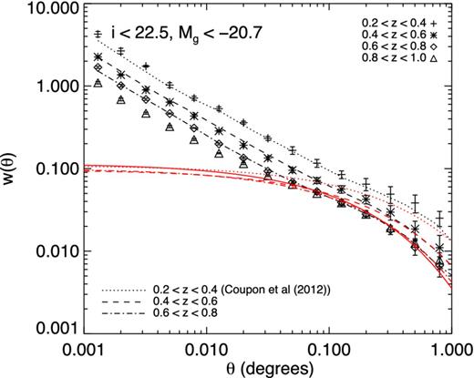
Comparison of measurements in this paper for the two-point correlation function (symbols) with those of Coupon et al. (dotted, dashed and dot–dashed black curves). The red curves represent the predictions of linear theory, as described in Section 4.2.3.
We next consider together the average two-point correlation (defined by equation 6) and the two-point correlation function measured for the same samples of galaxies, shown in the left-hand panel of Fig. 4.
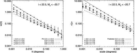
Left-hand panel: measurements of w(θ) in the four redshift bins. The lines are the fits obtained using a χ2 assuming a power law for the two-point correlation function. Right-hand panel: the averaged two-point correlation measured using counts in cells. The lines are the predicted values using equation (31) with the parameters of our w(θ) fit.
We see, as expected, the same behaviour as w(θ): at a fixed projected scale the correlation amplitude increases as the redshift decreases. We can also use this measurement to verify that the Landy & Szalay (1993) estimator measurements are consistent with our counts-in-cells measurements. To do this, we fit w(θ) by a simple power law w = Awθ1 − γ using a χ2 to estimate two parameters the amplitude Aw and the power γ. These fits are shown in the left-hand panel of Fig. 4. Our measurements are consistent with a constant or small variation (at the 1σ level) of the slope with redshift, as has been noted by previous authors (Coil et al. 2004; McCracken et al. 2008).
Comparing with a direct numerical integration, we found that this formula best approximates our measurements for 1.6 < γ < 2.0. The differences in |${\bar{\xi }}$| between the two methods range from 8.5 per cent for γ = 1.6 to less than 1 per cent for γ = 2. The results are presented in Table 4 and as the lines traced in the right-hand panel of Fig. 4.
Best-fitting slope γ values and χ2 derived using the fitting formula (25) to estimate |${\bar{\xi }}$| from w(θ).
| Redshift bin | Aw(1°) | γ | χ2 |
|---|---|---|---|
| 0.2 < z < 0.4 | 0.01 ± 0.001 | 1.9 ± 0.03 | 37.6 |
| 0.4 < z < 0.6 | 0.02 ± 0.004 | 1.8 ± 0.06 | 54.0 |
| 0.6 < z < 0.8 | 0.02 ± 0.002 | 1.7 ± 0.05 | 41.5 |
| 0.8 < z < 1.0 | 0.01 ± 0.002 | 1.65 ± 0.06 | 27.5 |
| Redshift bin | Aw(1°) | γ | χ2 |
|---|---|---|---|
| 0.2 < z < 0.4 | 0.01 ± 0.001 | 1.9 ± 0.03 | 37.6 |
| 0.4 < z < 0.6 | 0.02 ± 0.004 | 1.8 ± 0.06 | 54.0 |
| 0.6 < z < 0.8 | 0.02 ± 0.002 | 1.7 ± 0.05 | 41.5 |
| 0.8 < z < 1.0 | 0.01 ± 0.002 | 1.65 ± 0.06 | 27.5 |
4.2 Higher order moments
4.2.1 Comparison with SDSS DR7
We now consider measurements of the hierarchical moments. We first compare our CFHTLS measurements to measurements made in the SDSS Data Release 7 (SDSS-DR7) using an independently written counts-in-cells code (Ross et al. 2007). This software was used with the default configuration parameters proposed by the authors.
Since the SDSS and CFHTLS are very different surveys this comparison is only possible for the lowest redshift bin in the CFHTLS. We therefore selected galaxies with 0 < z < 0.4, 18 < r < 21 and Mr < −20.7 (comparable to Ross et al. 2007) and applied the same selection to galaxies in the SDSS. Our results are plotted in Fig. 5 where we show the hierarchical moments obtained from the four fields of the CFHTLS (solid lines) compared to measurements in the SDSS (dashed lines). For the CFHTLS, error bars are computed according to the method described in Section 3.4; for the SDSS, error bars were computed using a jackknife method (e.g. Scranton et al. 2002). For the detailed method see Ross et al. (2006).
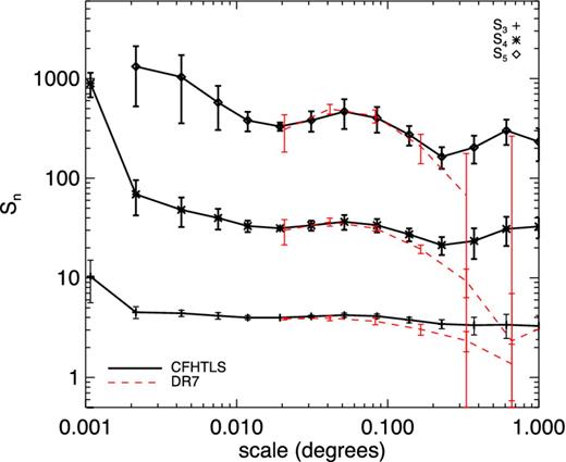
Hierarchical moments S3, S4 and S5 measured in the DR7 release of the SDSS for galaxies with 0 < z < 0.4, 18 < r < 21 and Mr < −20.7 (dashed lines) compared to measurements in the CFHTLS (solid lines).
As a consequence of the extremely fine pixelization grid used, we are able to measure our hierarchical moments to much smaller angular scales than in the SDSS (which would be computationally demanding for a large-area survey like the SDSS). Over the range of angular scales in common, the agreement between the CFHTLS and the SDSS measurements is excellent except at the largest scales. In this regime, BMW-PN better takes into account edge effects which explains the differences in the amplitude of the Sns. This is also reflected in our error bars that are smaller.
4.2.2 Field-to-field variations
Fig. 6 shows the third-order cumulant S3 as a function of scale in different redshift bins for the four different fields. At low redshifts, z ≲ 0.6, the dispersion between the four fields is low; however, above z ≃ 0.7 W3 becomes systematically higher than the other fields at all scales. At the highest redshifts, the difference between W3 and the other fields is significant. The same behaviour is observed for the other cumulants.
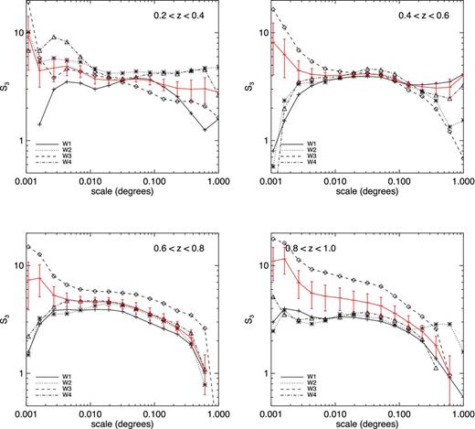
Measurements of S3 in the four fields of the CFHTLS in four redshift bins. The red line represents the combined S3 computed using the method described in Section 3.4. At low redshifts (z < 0.6) all the fields behave identically while at higher redshifts, S3 in W3 is systematically higher at all scales.
To illustrate this point Fig. 7 compares the hierarchical moments as a function of scale for the various redshift bins for the cases when all the fields are combined together and when W3 is excluded. The presence of W3 is in fact crucial because when it is included there clearly seems to be a redshift evolution of the hierarchical moments as indicated by the left-hand panel of Fig. 6, while removing W3 makes the redshift dependence insignificant as shown on the right-hand panel. We now investigate this effect in more detail.
Combined Sns as a function of angular scale in the four redshift bins when for all fields together (left-hand panel) and when W3 is excluded (right-hand panel). Negative values are not plotted.
The explanation of the behaviour of the cumulants in the highest redshift bin can be understood by considering Fig. 8 which shows the counts-in-cells distribution function for the combined fields, W1+W2+W3+W4, for W1+W2+W4 and for W3 alone. Clearly, the presence of W3 dominates and perturbs considerably the high end tail of PN(θ). A careful inspection of the W3 field reveals that this is due to the presence of several rich clusters in this field compared to the three other fields (see e.g. Colombi, Bouchet & Schaeffer 1994). Because of the finiteness of the sample there is a value Nmax(θ), above which PN(θ) becomes zero. This function Nmax(θ) obviously corresponds to the richest clusters of the sample: for instance a cell of size θ located in the densest part of one of the richest clusters of the sample should contain Nmax(θ) galaxies. Similarly, PN(θ) for N close to Nmax is entirely determined for a given smoothing scale θ by the density profile of a rich cluster of galaxies (cf. fig. 5 of Colombi et al. 1994).
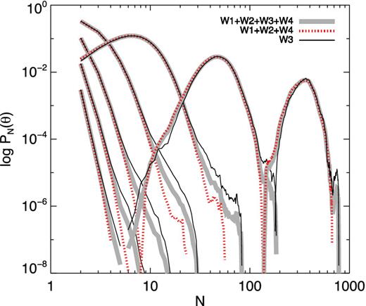
Counts-in-cells distribution function PN(θ) as a function of N in the last redshift bin 0.8 < z < 1.0. Three cases are considered: the combination W1+W2+W3+W4 using the weighting scheme as in equation (10) (thick grey curves), the combination W1+W2+W4 (red dotted curves) and W3 alone (solid black curves). Each curve corresponds to a different scale; for clarity only every second scale is shown.
To illustrate this point, Fig. 9 shows the largest cluster in W3 at 0.8 < z < 1.0 which has coordinates RA, |$\rm {Dec.}(\rm {J2000})=(216.5, 55.9)$| and the effect on S3 of masking it. As expected, removing the cluster greatly reduces the skewness over a large angular range. Indeed, moments of order k of the count probability are increasingly sensitive to the high-N tail of PN(θ) with increasing k. Removing the largest cluster reduces the high-N tail of PN(θ) and therefore reduces the skewness. This happens here only on a finite range of angular scales because, at smaller (larger) scales, one or several clusters with different concentration parameters from those of the one we selected dominate the high-N tail of the count probability. In fact, detailed examination of the four fields in the redshift bin 0.8 < z < 1 shows that there are four rich clusters in W3 and one in W1, which affect the cumulants and explains the discrepancy between W3 and the other fields. The sensitivity of higher order moments to the presence of rare, massive superstructures has been noted previously in other surveys (Croton et al. 2004).

A rich cluster in W3. Upper left-hand panel represents the distribution on the sky of galaxies in W3 for 0.8 < z < 1. The red square encloses the most prominent concentration from a visual inspection. The upper right-hand panel illustrates the effect of masking this concentration on S3 for W3 in the highest redshift bin. The lower left-hand panel shows a coloured image of the sky in the region delimited by the red square, which reveals a cluster of red galaxies. On the lower right-hand panel, the galaxies of the same region are represented in the same field with symbol colour representing redshift. We use a wider redshift bin (0.7 < z < 1.0) to be sure not to remove galaxies that belong to the cluster due to photometric redshift errors.
4.2.3 Statistical significance of measured field-to-field variations
To determine if the discrepancy between W3 and the three other fields is statistically significant we computed the theoretical errors on |$\bar{\xi }$|, S3 and S4 and compared them with errors estimated as described in Section 3.4. We did this using the Fortran for Cosmic Errors (force; Colombi & Szapudi 2001) package which exploits analytical calculations of Szapudi & Colombi (1996) and Szapudi et al. (1999) to provide quantitative estimates of these statistical errors due to the finiteness of the sample, given a number of input parameters that specify a prior model.
The calculation of |${\bar{\xi }}_S$| is however more involved. We do this using linear perturbation theory to derive a three-dimensional correlation function for a ΛCDM model. Then, we compute the angular two-point correlation function in the various redshift bins using equation (16), from which we can compute numerically the integral (26). This result is multiplied with the square of the bias between the galaxy and the dark matter distributions. To estimate this linear bias, we fit the measured two-point correlation function using the ‘halo model’ (Ma & Fry 2000; Peacock & Smith 2000; Scoccimarro et al. 2001; Cooray & Sheth 2002; Coupon et al. 2012). We find bias values of 1.17, 1.21, 1.27 and 1.37 with a typical error of ±0.01 for our four redshift intervals, from low to high redshift, respectively.
Fig. 10 compares the theoretical errors on |$\bar{\xi }$|, S3 and S4 derived using force to the measured weighted dispersion from the four fields. Three models are considered, in order to reflect uncertainties on the theory. These theoretical predictions are expected to be valid only when relative errors are small compared to unity as consequence of the propagation error technique used to derive it. Consequently, predictions at scales beyond 0| $_{.}^{\circ}$|1, where edge effects start to dominate in the theory are expected to be less accurate. With all these limitations in mind, one can see that the agreement between theory and measurements is excellent except in the redshift bin 0.6 < z < 0.8 where the relative error appears to be slightly underestimated or overestimated by the measurements when comparing to the theory for |$\bar{\xi }$| and the hierarchical moments, respectively.
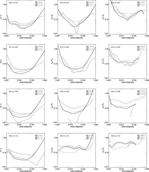
Comparison of theoretical errors to measured ones. Left to right: the relative error on the averaged two-point correlation function |$\bar{\xi }$| and hierarchical moments S3 and S4 measured from the data (red dot–dashed line) compared to theoretical models: Bernardeau & Schaeffer (1992) (BeS, solid line); Bernardeau (1994a, 1996) (PeR, dotted lines) and Szapudi & Szalay (1993a,b) (SzS, dashed lines). Each row represents a different redshift bin, from lowest on top to highest on bottom. Negative points are not plotted.
The remarkable agreement between theoretical errors derived using the standard ΛCDM model and the measured weighted dispersion between the four fields in the redshift bin 0.8 < z < 1 demonstrates that in fact W3 is not special from a statistical point of view and is fully consistent with our expected theoretical errors.
4.2.4 Redshift dependence of hierarchical moments and comparison with perturbation theory
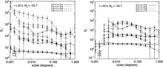
We now investigate the redshift dependence of the hierarchical moments. In Fig. 11 we show the hierarchical moments as functions of redshift for two typical angular scales: θ = 0| $_{.}^{\circ}$|012 which corresponds in practice to the non-linear regime at all redshifts and θ = 0| $_{.}^{\circ}$|23 which corresponds to the weakly non-linear regime. The top axis in Fig. 11 shows the comoving scales corresponding to θ = 0| $_{.}^{\circ}$|23 at each redshift interval.
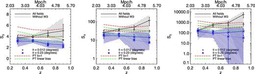
Left to right: evolution of S3, S4 and S5 with redshift at non-linear and weakly non-linear angular scales. The black symbols connected with solid lines and those linked with dotted lines correspond to θ = 0| $_{.}^{\circ}$|012 for all fields combined and without W3, respectively. The hashed grey region represents a 2σ confidence region around the solid black curves; for measurements θ = 0| $_{.}^{\circ}$|23 in blue. Perturbation theory predictions for θ = 0| $_{.}^{\circ}$|23 are given in green with linear bias and in red with b = 1. For each of these colours, there are two curves corresponding, respectively, to the 3D case (equations 27–29, lower curve) and the 2D case (equations 30–32, upper curve). The top axis shows the comoving scales corresponding to θ = 0| $_{.}^{\circ}$|23 at each redshift interval.
First, one can see that the Sn measurements without the W3 field are compatible within 2σ with those obtained using all fields at both angular scales. This confirms once more the conclusion of the previous section: the W3 field is not ‘special’ and this deviation is consistent with the observed errors. This demonstrates that the redshift evolution trend in the non-linear regime observed in left-hand panel of Fig. 7 and in Fig. 11 is indicative but inconclusive; this statement holds when angular scales are converted to megaparsec. From now on, we do not consider W3 separately and present results only for the full combination of the four fields.
Fig. 12 shows the hierarchical moments in three-dimensional space as a function of physical scale after applying the transformation described in Section 3.5. The measurements show the same behaviour as before, i.e. a plateau at small scales corresponding to the highly non-linear regime, and then a second, lower plateau, at large scales corresponding to the weakly non-linear regime. At scales ∼10 Mpc, we start to be sensitive to finite size effects as we approach the size of the fields.
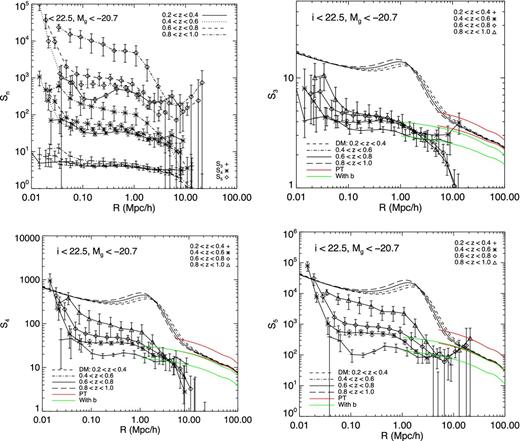
Deprojected Sns in the four redshift bins, together on the same plot (upper left-hand panel) and individually (three remaining panels). The dashed and dot–dashed black curves on each panel give dark matter halo model prediction. The coloured lines represent pure perturbation theory predictions using equations (27)–(29) (lower curves) and equations (30)–(32) (upper curves) in two cases: one without bias and one with the most extreme value of linear bias, b = 1.37, found in the last redshift bin.
In his analysis, Bernardeau (1995) showed that the small angle approximation also has its limits and the correct value lies between the 3D and the 2D predictions. It is probably closer to the latter one in the angular range probed by our measurements. Therefore, our comparisons to perturbation theory consider both the Σn and the |$S_{n}^{\rm PT}$| as bracketing the true prediction from perturbation theory.
In Figs 11 and 12 we see that perturbation theory predictions (shown as the red curves in Figs 11 and 12) lie above the measurements at large scales; however, these theoretical predictions do not take into account of linear bias between the galaxy distribution and the total matter distribution. As a consequence of this the measurements are slightly below the theoretical predictions.
Finally, in Fig. 12, the full halo-model predictions for the dark matter are given using the method of Fry et al. (2011). What is interesting to notice here is that the halo model predictions and measurements are consistent concerning the location of the transition between the weakly non-linear regime and the highly non-linear regime.
5 CONCLUSIONS
We have measured the hierarchical moments of the galaxy distribution S3, S4 and S5 in a volume-limited sample of more than one million galaxies spanning the redshift range z ∼ 1 to z ∼ 2. Our measurements were made in the latest release of the CFHTLS-Wide and cover an effective area of |$133 \, \rm {deg}^2$|.
We are able for the first time to make robust measurements of the evolution of the hierarchical moments as functions of redshift within a large range of angular scales. The survey consists of four independent fields, allowing us to estimate the cosmic variance at each bin and angular scale.
Our main results are as follows.
In the redshift bin 0.2 < z < 0.4 for a sample with the same cut in absolute magnitude, our results are in excellent agreement with the SDSS demonstrating that our survey is a fair sample of the Universe.
This is confirmed by a comparison of the field to field scatter of the variance of counts in cells and the predicted hierarchical moments with the analytic ‘cosmic errors’ predicted by Szapudi & Colombi (1996) and Szapudi et al. (1999).
The hierarchical moments that we measure show two regimes separated by a transition region: first, a plateau at small scales (|${\lesssim } 1 \, h^{-1} \, \rm {Mpc}$|) corresponding to the highly non-linear regime, and then the data tend to another lower plateau at large scales (|${\gtrsim } 7 h^{-1} \, \rm {Mpc}$|) corresponding to the weakly non-linear regime.
At non-linear scales, the amplitude of the hierarchical moments increases with redshift: however, a more accurate error analysis demonstrates that our results are also consistent with no redshift evolution within 2σ.
In the weakly non-linear regime measurements are marginally consistent with the perturbation theory predictions when a linear bias term (measured from our data) is taken into account. However, these predictions seem to slightly overpredict our measurements, which suggests the existence of higher order bias terms corrections (Fry & Gaztanaga 1993) which will be considered in a future work.
The position of the transition between the non-linear and the weakly non-linear regime |$1 \lesssim R \lesssim 10 \, h^{-1} \, \rm {Mpc}$| is fully compatible with halo model predictions.
A robust conclusion concerning the redshift evolution of the hierarchical moments in the non-linear regime, and the corresponding implications for galaxy formation and evolution, is challenging. This is because the richest clusters in our sample can dramatically influence higher order measurements. A complete understanding of this effect will require a detailed modelling of the counts-in-cells probability using the halo model formalism, taking into account the halo mass of the most massive structure in our survey as well as a full error analysis including covariances. This will be the subject of a subsequent work.
We would like to thank Ashely Ross for providing his code to calculate the counts in cells for SDSS DR7 and the associated catalogues and advice. We acknowledge Raphael Sadoun for his useful help and suggestions. HJM acknowledges support from the ‘Programme national cosmologie et galaxies’. JNF thanks the IAP for hospitality during his work. HJM and MW acknowledge the use of Terapix computing resources.
Based on observations obtained with MegaPrime/MegaCam, a joint project of CFHT and CEA/IRFU, at the Canada–France–Hawaii Telescope (CFHT) which is operated by the National Research Council (NRC) of Canada, the Institut National des Science de l'Univers of the Centre National de la Recherche Scientifique (CNRS) of France and the University of Hawaii. This work is based in part on data products produced at Terapix available at the Canadian Astronomy Data Centre as part of the Canada–France–Hawaii Telescope Legacy Survey, a collaborative project of NRC and CNRS.
Hence, this is only an approximate implementation of the jackknife with additional edge effects due to the fact that counts in cells are measured in each subfield independently.
At least in the Poisson approximation, when xi = F1 measured in field i.
REFERENCES
APPENDIX A: WEIGHTED STATISTICS
In this appendix, we describe the way we estimate errors of the combined quantities.
APPENDIX B: Sn MEASUREMENTS
The Sn measurements are presented below.
Measured Sn and their error bars in the bins 0.2 < z < 0.4, 0.4 < z < 0.6, 0.6 < z < 0.8 and 0.8 < z < 1. The first column refers to the angular size of the square cells used to perform the measurements. The next columns display successively S3 and its error bars, S4 and its error bars and S5 and its error bars. The counts-in-cells method used to perform the measurements is described in Section 3.3. The way the four fields are combined and the corresponding error bars are computed is detailed in Section 3.4.
| θ | S3 | |$\sigma _{S_{3}}$| | S4 | |$\sigma _{S_{4}}$| | S5 | |$\sigma _{S_{5}}$| |
|---|---|---|---|---|---|---|
| 0.2 < z < 0.4 | ||||||
| 0.0011 | 9.34 | 4.84 | −8.92 | 3.96 | −15.5 | 7.99 |
| 0.0016 | 4.45 | 1.33 | −4.29 | 0.80 | −6.8 | 1.85 |
| 0.0027 | 4.72 | 1.21 | 54.7 | 42.7 | −84.0 | 44.7 |
| 0.0043 | 4.90 | 0.91 | 58.6 | 38.3 | 625 | 735 |
| 0.0070 | 4.39 | 0.55 | 43.6 | 15.0 | 468 | 262 |
| 0.0118 | 3.73 | 0.38 | 26.3 | 6.22 | 166 | 73.1 |
| 0.0193 | 3.62 | 0.21 | 23.6 | 2.91 | 158 | 26.4 |
| 0.0317 | 3.67 | 0.14 | 24.8 | 1.83 | 208 | 30.3 |
| 0.0516 | 3.71 | 0.22 | 27.6 | 4.12 | 310 | 84.2 |
| 0.0849 | 3.59 | 0.31 | 25.8 | 5.11 | 278 | 83.2 |
| 0.1392 | 3.30 | 0.40 | 21.7 | 5.44 | 216 | 68.8 |
| 0.2273 | 3.06 | 0.46 | 17.3 | 5.33 | 135 | 48.9 |
| 0.3729 | 2.99 | 0.65 | 17.9 | 7.01 | 138 | 51.2 |
| 0.6105 | 3.02 | 0.81 | 21.8 | 8.96 | 198 | 80.7 |
| 1.0001 | 2.81 | 0.63 | 15.5 | 5.60 | 75.7 | 53.5 |
| 0.4 < z < 0.6 | ||||||
| 0.0011 | 8.18 | 4.10 | 1007 | 435 | 89 701 | 30 529 |
| 0.0016 | 6.27 | 2.45 | 228 | 101 | 8823 | 3051 |
| 0.0027 | 4.46 | 1.03 | 61.1 | 32.1 | 1157 | 645 |
| 0.0043 | 4.12 | 0.54 | 42.3 | 15.8 | 656 | 343 |
| 0.0070 | 4.01 | 0.27 | 38.9 | 7.14 | 579 | 150 |
| 0.0118 | 4.03 | 0.15 | 38.4 | 4.11 | 611 | 131 |
| 0.0193 | 4.10 | 0.09 | 37.9 | 3.40 | 557 | 115 |
| 0.0317 | 4.17 | 0.14 | 38.8 | 3.50 | 547 | 91.4 |
| 0.0516 | 4.09 | 0.13 | 36.9 | 2.93 | 484 | 70.3 |
| 0.0849 | 3.72 | 0.12 | 28.6 | 2.89 | 299 | 56.4 |
| 0.1392 | 3.30 | 0.10 | 20.0 | 1.86 | 145 | 18.8 |
| 0.2273 | 3.15 | 0.17 | 17.3 | 2.81 | 88.5 | 28.2 |
| 0.3729 | 3.07 | 0.35 | 13.1 | 5.85 | −10.1 | 41.4 |
| 0.6105 | 3.12 | 0.60 | 2.94 | 8.54 | −249 | 43.0 |
| 1.0001 | 4.01 | 0.87 | −5.00 | 11.4 | −595 | 241 |
| 0.6 < z < 0.8 | ||||||
| 0.0011 | 7.32 | 3.43 | 455 | 232 | 33 737 | 13 985 |
| 0.0016 | 7.64 | 2.53 | 220 | 93.4 | 8710 | 2910 |
| 0.0027 | 5.30 | 1.08 | 79.8 | 33.9 | 1832 | 916 |
| 0.0043 | 4.86 | 0.70 | 61.8 | 23.2 | 1151 | 668 |
| 0.0070 | 4.64 | 0.54 | 54.7 | 17.4 | 1025 | 541 |
| 0.0118 | 4.62 | 0.45 | 51.0 | 12.6 | 910 | 360 |
| 0.0193 | 4.60 | 0.44 | 50.6 | 10.7 | 885 | 260 |
| 0.0317 | 4.40 | 0.44 | 46.6 | 9.81 | 769 | 214 |
| 0.0516 | 4.05 | 0.49 | 40.0 | 11.5 | 620 | 255 |
| 0.0849 | 3.58 | 0.48 | 29.1 | 10.3 | 373 | 206 |
| 0.1392 | 3.13 | 0.45 | 21.1 | 8.56 | 203 | 144 |
| 0.2273 | 2.67 | 0.36 | 15.1 | 6.34 | 106 | 108 |
| 0.3729 | 2.13 | 0.41 | 9.87 | 6.38 | 65.7 | 99 |
| 0.6105 | 1.06 | 0.43 | 3.41 | 3.25 | 141 | 53 |
| 1.0001 | −0.69 | 0.33 | −5.60 | 2.64 | 221 | 588 |
| 0.8 < z < 1.0 | ||||||
| 0.0011 | 11.0 | 3.75 | 365 | 136 | −819 | 226 |
| 0.0016 | 11.5 | 3.18 | 483 | 147 | 16 011 | 3325 |
| 0.0027 | 6.96 | 2.01 | 223 | 102 | 10 415 | 4062 |
| 0.0043 | 5.54 | 1.55 | 161 | 84.7 | 8770 | 4397 |
| 0.0070 | 5.20 | 1.41 | 135 | 71.8 | 6970 | 3767 |
| 0.0118 | 5.01 | 1.19 | 117 | 56.4 | 5579 | 2893 |
| 0.0193 | 4.77 | 1.02 | 96.0 | 42.0 | 3757 | 1829 |
| 0.0317 | 4.54 | 0.93 | 90.5 | 40.2 | 3664 | 1865 |
| 0.0516 | 4.23 | 0.85 | 79.9 | 37.7 | 3271 | 1836 |
| 0.0849 | 3.60 | 0.62 | 47.5 | 21.7 | 1352 | 792 |
| 0.1392 | 2.99 | 0.44 | 24.9 | 10.5 | 403 | 249 |
| 0.2273 | 2.45 | 0.34 | 13.9 | 5.50 | 142 | 90.5 |
| 0.3729 | 1.81 | 0.39 | 7.74 | 5.89 | 131 | 109 |
| 0.6105 | 0.99 | 0.47 | −1.92 | 8.71 | 211 | 225 |
| 1.0001 | −0.36 | 0.95 | −15.02 | 17.0 | 508 | 575 |
